Fusion and breakup in the reactions of ^6,7Li and ⁹Be

Abstract

We develop a three body classical trajectory Monte Carlo (CTMC) method to dicsuss the effect of the breakup process on heavy-ion fusion reactions induced by weakly bound nuclei. This method follows the classical trajectories of breakup fragments after the breakup takes place, and thus provides an unambiguous separation between complete and incomplete fusion cross sections. Applying this method to the fusion reaction ⁶Li + ²⁰⁹Bi, we find that there is a significant contribution to the total complete fusion cross sections from the process where all the breakup fragments are captured by the target nucleus (i.e., the breakup followed by complete fusion).

1 Introduction

The fusion reactions of neutron-rich nuclei around the Coulomb barrier provide a good opportunity to study the interplay between quantum tunneling and the breakup process. An important question here is: does the breakup process influence fusion reactions in a similar way as the inelastic process, which leads to subbarrier enhancement [1] of fusion cross sections over predictions for a single barrier? In addressing this question, measurements with weakly bound stable nuclei, such as ⁹Be, ⁶Li, and ⁷Li, have been proved to be useful[2, 3, 4]. These beams are currently much more intense than radioactive beams, allowing more precise and extensive experimental studies. Also, these nuclei predominantly break up into charge fragments (⁹Be $\to$ 2$\alpha+n$ or $\alpha+^{5}$He, ⁷Li $\to$ $\alpha+t$, and ⁶Li $\to$ $\alpha+d$), which are more easily detected. This allows a clean separation of the products of complete fusion from those of incomplete fusion, where only a part of the projectile is captured.

To describe the effect of breakup on fusion reactions theoretically, a model has to take into account the following three different processes: (i) the projectile as a whole is captured by the target, (ii) only one of the breakup fragments is captured, (iii) all the breakup fragments are absorbed after the breakup takes place near the target nucleus. Process (ii) is referred to as an incomplete fusion reaction, while both of processes (i) and (iii) lead to complete fusion. Calculations based on the continuum-discretized coupled-channels method may account for the total fusion cross section (the sum of all the processes) and/or the separate contribution of process (i)[5, 6], but it is not easy to compute cross sections for process (iii), that is, the breakup followed by complete fusion. In order to model this process, we need to follow the trajectories of the breakup fragments to determine whether one or both fragments are captured by the target nucleus. In this contribution, we present such a model[3], where many classical trajectories are sampled by the Monte Carlo method to compute the total complete fusion cross section. We note that a very similar model, called the three-body classical trajectory Monte Carlo (CTMC) method, has been developed in the field of atomic and molecular physics, and has been successfully applied to ion-atom ionization and charge transfer collisions [7, 8, 9].

2 Three-body classical trajectory Monte Carlo (CTMC) model

Let us assume the following Hamiltonian for a reaction of a projectile nucleus which consists of two cluster fragments $P_{1}$ and $P_{2}$,

$$H=\frac{\mbox{\boldmath$p$}_{1}^{2}}{2m_{1}}+\frac{\mbox{\boldmath$p$}_{2}^{2}}{2m_{2}}+\frac{\mbox{\boldmath$p$}_{T}^{2}}{2m_{T}}+V_{12}(\mbox{\boldmath$r$}_{1}-\mbox{\boldmath$r$}_{2})+V_{1T}(\mbox{\boldmath$r$}_{1}-\mbox{\boldmath$r$}_{T})+V_{2T}(\mbox{\boldmath$r$}_{2}-\mbox{\boldmath$r$}_{T}),$$ (1)

where $\mbox{\boldmath$p$}_{1}$, $\mbox{\boldmath$p$}_{2}$, and $\mbox{\boldmath$p$}_{T}$ are the momenta of fragment $P_{1}$, $P_{2}$, and of the target, respectively. $\mbox{\boldmath$r$}_{1}$, $\mbox{\boldmath$r$}_{2}$, and $\mbox{\boldmath$r$}_{T}$ are the corresponding coordinates. The idea of the three-body classical trajectory model is to solve this Hamiltonian classically in the two-dimensional ($x,y$) plane [3]. We assume that at $t$=0 the target is at rest at the origin, while the center of mass of the projectile is at $(x,y)=(R_{\rm max},b)$ moving towards the $-x$ direction. Here, $R_{\rm max}$ is some large number, while $b$ is the impact parameter. The relative motion between the projectile fragments is confined at $t=0$ inside the potential $V_{12}$ at the energy corresponding to the breakup $Q$-value, $Q_{\rm bu}$, with a random orientation $\theta$ with respect to the $x$ axis. The initial conditions thus read,

$$x_{1}(0) = R_{\rm max}-\frac{m_{2}}{m_{1}+m_{2}}\,r_{0}\,\cos\theta,~{}~{}~{}~{}~{}y_{1}(0)=b+\frac{m_{2}}{m_{1}+m_{2}}\,r_{0}\,\sin\theta,$$ (2)

$$x_{2}(0) = R_{\rm max}+\frac{m_{1}}{m_{1}+m_{2}}\,r_{0}\,\cos\theta,~{}~{}~{}~{}~{}y_{2}(0)=b-\frac{m_{1}}{m_{1}+m_{2}}\,r_{0}\,\sin\theta,$$ (3)

$$v_{x1}(0) = -v_{\rm lab}-\frac{1}{2m_{1}}p_{\rm rel}\cos\theta,~{}~{}~{}~{}~{}~{}~{}~{}v_{y1}(0)=\frac{1}{2m_{1}}p_{\rm rel}\sin\theta,$$ (4)

$$v_{x2}(0) = -v_{\rm lab}+\frac{1}{2m_{2}}p_{\rm rel}\cos\theta,~{}~{}~{}~{}~{}~{}~{}~{}v_{y2}(0)=-\frac{1}{2m_{2}}p_{\rm rel}\sin\theta,$$ (5)

$$x_{T}(0) = y_{T}(0)=v_{xT}(0)=v_{yT}(0)=0,$$ (6)

where

$$v_{\rm lab}=\sqrt{\frac{2}{m_{1}+m_{2}}[E_{\rm lab}-V_{1T}(r_{1T}(0))-V_{2T}(r_{2T}(0))]},$$ (7)

is the initial velocity for the center of mass of the projectile, and $p_{\rm rel}=\sqrt{2\mu[Q_{\rm bu}-V_{12}(r_{12}(0))]}$ with $\mu=m_{1}m_{2}/(m_{1}+m_{2})$. The value of $r_{0}$ is restricted to $0\leq r_{0}\leq r_{t}$, where $r_{t}$ satisfies $V_{12}(r_{t})=Q_{\rm bu}$.

With these initial conditions, we solve the Newtonian equations to follow the time evolution of the trajectories for each particle, $x_{i}(t),y_{i}(t),v_{xi}(t)$, and $v_{yi}(t),(i=1,2,T)$. At each time, we monitor the relative distance between the particles. We assume that the projectile fragment $P_{i}~{}(i=1,2)$ is absorbed by the target nucleus when the relative distance between the fragment and the target is smaller than $r_{iT}<1.1(A_{i}^{1/3}+A_{T}^{1/3})$ fm, and that the breakup occurs when the relative distance between $P_{1}$ and $P_{2}$ is larger than the barrier radius for the potential $V_{12}$. By sampling many trajectories for random values of $r_{0}$ and $\theta$ with the Monte Carlo method, we calculate partial cross sections for a given impact parameter $b$. Total cross sections are then obtained by integrating them over the value of $b$.

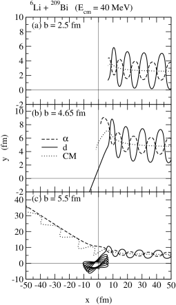
Figure 1: Examples of classical trajectories for the ⁶Li+²⁰⁹Bi reaction. Fig. 1(a), (b), and (c) are for the impact parameter $b$=2.5, 4.65, and 5.5 fm at $E_{cm}$=40 MeV, respectively. The dashed and the solid lines correspond to the trajectories for the $\alpha$ particle and deuteron, respectively, while the dotted line is for the center of mass of the projectile fragments.

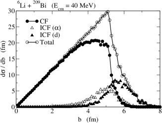
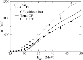
Figure 2: The partial fusion cross sections $d\sigma/db$ for the ⁶Li+²⁰⁹Bi reaction at $E_{cm}$=40 MeV obtained with the three-body classical trajectory Monte Carlo method.

Figure 3: The complete fusion (CF) and the incomplete fusion (ICF) cross sections for the ⁶Li+²⁰⁹Bi reaction. The experimental data are taken from Ref. [3].

3 Application to ⁶Li + ²⁰⁹Bi reaction

We now apply the three-body classical trajectory Monte Carlo method to the ⁶Li + ²⁰⁹Bi system and discuss the effect of breakup of ⁶Li into $d+\alpha$ on the fusion reaction near the Coulomb barrier. We assume the Woods-Saxon form in calculating $V_{12},V_{1T}$, and $V_{2T}$, using the same values for the parameters as in Refs. [10, 11]. We take $R_{\rm max}$ = 200 fm. Fig. 1(a) – 1(c) shows sample trajectories at $E_{\rm cm}$ = 40 MeV. These are for $b$=2.5, 4.65, and 5.5 fm, respectively. For relatively small values of the impact parameter (Fig. 1(a)), the projectile nucleus ⁶Li is captured by the target before breaking up into $\alpha$ and $d$, leading to complete fusion. For $b$=5.5 fm (Fig. 1(c)), only the deuteron is captured while the alpha particle escapes from the target. This is an example of incomplete fusion. For intermediate values of $b$, breakup takes place near the target, but both of the breakup fragments get absorbed (Fig. 1(b)). This is breakup followed by complete fusion. Figure 2 shows the partial fusion cross sections for these processes as a function of the impact parameter, for $E_{cm}$=40 MeV.

Figure 3 shows fusion cross sections as a function of energy in the center of mass frame. The dotted line denotes the sum of complete and incomplete fusion cross sections. The dashed line indicates the absorption of the whole projectile from the bound states, while the solid line shows the total complete fusion cross sections. The difference between the solid and the dashed line thus represents the contribution from breakup followed by fusion of both fragments. This makes a significant contribution to complete fusion at energies above the barrier.

4 Summary

We present a three body classical trajectory Monte Carlo method for fusion of weakly bound nuclei. Applying this method to the ⁶Li + ²⁰⁹Bi reaction, we have demonstrated that there is a significant contribution of breakup followed by complete fusion to the total complete fusion cross sections. This process has not been considered in any coupled-channels calculations so far, and the present result suggests that a consistent definition of complete fusion is necessary when one compares experimental data with theoretical calculations.

References

- [1] M. Dasgupta, et al., Annu. Rev. Nucl. Part. Sci. 48 (1998) 401.
- [2] M. Dasgupta et al., Phys. Rev. Lett. 82 (1999) 1395.
- [3] M. Dasgupta et al., Phys. Rev. C66 (2002) 041602(R).
- [4] I. Padron et al., Phys. Rev. C66 (2002) 044608.
- [5] K. Hagino, A. Vitturi, C.H. Dasso, and S.M. Lenzi, Phys. Rev. C61 (2000) 037602.
- [6] A. Diaz-Torres and I.J. Thompson, Phys. Rev. C65 (2002) 024606.
- [7] R. Abrines and I.C. Percival, Proc. Phys. Soc. 88 (1966) 861.
- [8] J.S. Cohen, Phys. Rev. A27 (1983) 167.
- [9] J. Fiol, C. Courbin, V.D. Rodriguez, and R.O. Barrachina, J. Phys. B33 (2000) 5343.
- [10] I.J. Thompson and M.A. Nagarajan, Phys. Lett. 106B (1981) 163.
- [11] G. Goldring, et al., Phys. Lett. 32B (1970) 465.