Sum rules and short-range correlations in nuclear matter at finite temperature

Abstract

The nucleon spectral function in nuclear matter fulfills an energy weighted sum rule. Comparing two different realistic potential, these sum rules are studied for Green’s functions that are derived self-consistently within the $T$ matrix approximation at finite temperature.

The microscopic study of the single-particle properties in nuclear matter requires a rigorous treatment of the nucleon-nucleon (NN) correlations bal1 ; her1 . In fact, the strong short-range and tensor components, which are needed in realistic NN interactions to fit the NN scattering data, lead to important modifications of the nuclear wave function. A clear indication of the importance of correlations is provided by the observation that a simple Hartree-Fock calculation for nuclear matter at the empirical saturation density using such realistic NN interactions typically results in positive energies rather than the empirical value of $-16\,\mbox{MeV}$ per nucleon her1 .

Correlations do not only manifest themselves in the bulk properties but also modify the single-particle properties in a substantial way. Several recent calculations have shown without ambiguity how the NN correlations produce a partial occupation of the single particle states which would be fully occupied in a mean field description and a wide distribution in energy of the single particle strength. These two features have also been empirically founded in the analysis of the (e,e’p) nucleon knock-out reactions exp1 . The theoretical studies have been conducted both in finite nuclei her2 and also in nuclear matter fan1 ; ram1 ; dick1 .

An optimal tool to study the single particle properties is provided by the self-consistent Green’s function technique (SCGF) dick2 . This method gives direct access to the single particle spectral function, which should be self-consistently determined at the same time than the effective interactions between the nucleons in the medium. Enormous progress in the SCGF applications to nuclear matter have been reported in the last years, both at zero dick1 and finite temperature boz1 ; boz2 ; fri03 .

The efforts at $T=0$ have mainly been addressed to provide the appropriate theoretical background for the interpretation of the (e,e’p) experiments while the investigation at finite $T$ are mainly oriented to describe the nuclear medium in astrophysical environments or to the interpretation of the dynamics of heavy ion collisions.

In any case, the key quantity is the single-particle spectral function, i.e. the distribution of strength in energy when one adds or removes a particle of the system with a given momentum. A possible way to analyze the single-particle spectral function is by means of the energy weighted sum rules. They are well established in the literature and have been numerically analyzed in the case of zero temperature pol94 .

The analysis of the energy weighted sum-rules can give useful insights not only on the numerical accuracy of the many-body approach used to calculate them but also can help to understand the properties and structure of the NN potential.

This paper is devoted to study the physical implications of the fulfillment of these sum rules for single particle spectral functions in nuclear matter at finite $T$. This investigation is based on the framework of SCGF employing a fully self-consistent ladder approximation in which the complete spectral function has been used to describe the intermediate states in the Galistkii-Feynman equation.

After a brief summary of the definitions of the single-particle spectral function, we give a simple derivation of the sum rules. Then we analyze the results for two types of realistic potentials, the CDBONN and the Argonne V18, and discuss the different behaviors based on the different strength of the short-range and tensor components of both potentials.

For a given Hamiltonian $H$, the Green’s function for a system at finite temperature can be defined in a grand-canonical formulation:

$${\mathrm{i}}g({\mathbf{k}}t;{\mathbf{k}}^{\prime}t^{\prime})={\mathrm{Tr}}\{\rho\,{\mathbf{T}}[a^{\phantom{\dagger}}_{\mathbf{k}}(t)a^{\dagger}_{{\mathbf{k}}^{\prime}}(t^{\prime})]\}.$$ (1)

$\mathbf{T}$ is the time ordering operator that acts on a product of Heisenberg field operators $a_{\mathbf{k}}(t)=e^{{\mathrm{i}}tH}a_{\mathbf{k}}e^{-{\mathrm{i}}tH}$ in such a way that the field operator with the largest time argument $t$ is put to the left. The trace is to be taken over all energy eigenstates and all particle number eigenstates of the many body system, weighted by the statistical operator,

$$\rho=\frac{1}{Z}\,{e^{-\beta(H-\mu N)}}.$$ (2)

$\beta$ and $\mu$ denote the inverse temperature and the chemical potential, respectively. N is the operator that counts the total number of particles in the system,

$$N=\sum_{\mathbf{k}}a_{\mathbf{k}}^{\dagger}(t)a_{\mathbf{k}}^{\phantom{\dagger}}(t)$$ (3)

$N$ is independent of time, since it commutes with $H$. The normalization factor in Eq. (2) is given by the grand partition function of statistical mechanics,

$$Z={{\mathrm{Tr}}\,e^{-\beta(H-\mu N)}}.$$ (4)

For a homogeneous system, the Green’s function is diagonal in momentum space and depends only on the absolute value of ${\mathbf{k}}$ and on the difference $\tau=t^{\prime}-t$. Starting from the definition of the Green’s function, we first focus on the case $\tau>0$. In order to recover the expression for the ensemble average of the occupation number $n(k)$ for $\tau=0^{+}$, the following definition of the correlation function, $g^{<}$, includes an additional factor of $-{\mathrm{i}}$ with respect to the definition of the Green’s function $g$,

$$g^{<}(k,\tau)={\mathrm{Tr}}\{\rho\,e^{{\mathrm{i}}\tau H}a^{\dagger}_{{\mathbf{k}}}e^{-{\mathrm{i}}\tau H}a^{\phantom{\dagger}}_{\mathbf{k}}\}.$$ (5)

$g^{<}(k,\tau)$ can be expressed as a Fourier integral over all frequencies,

$$g^{<}(k,\tau)=\int_{-\infty}^{+\infty}\frac{{\mathrm{d}}\omega}{2\pi}\,e^{-{\mathrm{i}}\omega\tau}A^{<}(k,\omega)$$ (6)

if $A^{<}(k,\omega)$ is defined by kraeft :

$$A^{<}(k,\omega)=2\pi\sum_{nm}\frac{e^{-\beta(E_{m}-\mu N_{m})}}{Z}\left|\left<\Psi_{n}|a_{k}|\Psi_{m}\right>\right|^{2}\delta(\omega-(E_{m}-E_{n})).$$ (7)

This can be easily checked by inserting the eigenstates $\left|\Psi_{n}\right>$ into the expression of the trace in Eq. (5). It is important to note that $\left|\Psi_{n}\right>$ are simultaneous eigenstates of both the number operator and the Hamiltonian.
A similar analysis can be conducted for $\tau<0$, yielding a function

$$A^{>}(k,\omega)=e^{\beta(\omega-\mu)}A^{<}(k,\omega).$$ (8)

The spectral function at finite temperature is defined as the sum of the two positive functions, $A^{<}$ and $A^{>}$,

$$A(k,\omega)=A^{<}(k,\omega)+A^{>}(k,\omega).$$ (9)

Expression (7), for $A^{<}$, can be compared to the result for the hole spectral function at zero temperature, that was reported in Ref pol94 ,

$$A_{h}(k,\omega)=2\pi\sum_{n}\left|\left<\Psi_{n}^{A-1}|a_{k}|\Psi_{0}^{A}\right>\right|^{2}\delta(\omega-(E_{0}^{A}-E_{n}^{A-1})),$$ (10)

where $\left|\Psi_{0}^{A}\right>$ is the ground state of an $A$ particle system and $\left|\Psi_{n}^{A-1}\right>$ labels the excited energy eigenstates of a system that contains one particle less. The physical interpretation of the hole spectral function in a system at zero temperature is the following: $A_{h}(k,\omega)$ is the probability to remove a particle from the ground state of the $A$-body system, such, that the residual system is left with an excitation energy $E^{A-1}_{n}=E^{A}_{0}-\omega$. $E^{A}_{0}$ is the ground state energy of the $A$ particle system. It is clear that the lowest possible energy of the final state is the ground state energy of the $A-1$ particle system, so that there is an upper limit for the hole spectral function at $\omega=E_{0}^{A}-E_{0}^{A-1}=\mu$. In a similar fashion, the particle spectral function $A_{p}$ can be defined as the probability to attach a further nucleon to the system in such a way, that the excitation energy of the compound system with respect to the ground state energy of the initial system is $\omega=E^{A+1}-E_{0}^{A}$. In this case, one can argue that, to add a further particle, one has to pay at least the chemical potential, so that $\mu$ is a lower bound for $\omega$. At zero temperature, this behavior causes a complete separation of the particle and the hole spectral function.

The situation is quite different in a grand-canonical formulation at finite temperature To illustrate these changes, the full spectral function A, as well as $A^{>}$ and $A^{<}$ are shown in Fig. 1 for three momenta around the Fermi momentum of a zero temperature system at the same density, $\rho=0.2\,\mbox{fm}^{-3}$. Numerical values for the integrated strength of $A^{<}$ are listed in Table 1. Since thermally excited states $\left|\Psi_{m}\right>$ are always included in the grand-canonical ensemble average according to their weight factor $e^{-\beta(E_{m}-\mu N_{m})}$, one can take out a particle from a thermally excited state and end up in a weakly excited state close to the ground state of the residual system. This leads to a contribution to $A^{<}$ for an energy $\omega$ larger than $\mu$. Also one has to keep in mind that we are considering a grand-canonical average. This implies that with the appropriate weight one also considers systems with a density larger than the mean value. For those systems, a removal of particles from states with single-particle energies above $\mu$ will also be possible.

Similarly, a particle can be added to a thermally excited state, leaving the compound system in a state close to its ground state, so that $A^{>}(k,\omega)$ extends to the region below $\mu$. In any case, there is no longer a separation between $A^{>}$ and $A^{<}$, and the maxima of both functions can even coincide. This is also quite obvious from the relation (8).

For the $T$ matrix approximation to the self energy reported in fri03 , one can determine the single-particle Green’s function as the solution of Dyson’s equation for any complex value of the frequency variable $z$,

$$g(k,z)=\frac{1}{z-\frac{k^{2}}{2m}-\Sigma(k,z)}.$$ (11)

Using the analytical properties of the finite temperature Green’s function along the imaginary time axis, an important relation between the spectral function and the Green’s function can be derived and analytically continued to slightly complex values kad62 :

$$g(k,\omega+{\mathrm{i}}\eta)=\int_{-\infty}^{+\infty}\frac{{\mathrm{d}}\omega^{\prime}}{2\pi}\,\frac{A(k,\omega)}{\omega-\omega^{\prime}+{\mathrm{i}}\eta}.$$ (12)

One can extract sum rules from the asymptotic behavior at large $\omega$ by expanding the real part of both expressions for the Green’s function, Eqs. (11) and (12), in powers of $\frac{1}{\omega}$. This yields

$${\mathrm{Re}}\,g(k,\omega)=\frac{1}{\omega}\left\{1+\frac{1}{\omega}\left[\frac{k^{2}}{2m}+\lim_{\omega\rightarrow\infty}{\mathrm{Re}}\,\Sigma(k,\omega)\right]+\cdots\right\}$$ (13)

and

$${\mathrm{Re}}\,g(k,\omega)=\frac{1}{\omega}\left\{\int_{-\infty}^{+\infty}{\mathrm{d}}\omega^{\prime}\,A(k,\omega^{\prime})+\frac{1}{\omega}\int_{-\infty}^{+\infty}{\mathrm{d}}\omega^{\prime}\,\omega^{\prime}A(k,\omega^{\prime})+\cdots\right\}.$$ (14)

By comparing the first two expansion coefficients, one finds the $m_{0}$ and the $m_{1}$ sum rules,

$$\int_{-\infty}^{+\infty}\frac{{\mathrm{d}}\omega}{2\pi}A(k,\omega)=1,$$ (15)

and

$$\int_{-\infty}^{+\infty}\frac{{\mathrm{d}}\omega}{2\pi}A(k,\omega)\omega=\frac{k^{2}}{2m}+\lim_{\omega\rightarrow\infty}{\mathrm{Re}}\,\Sigma(k,\omega)$$ (16)

Similar sum rules can be obtained from the higher order terms, as it was done in Ref. pol94 for $m_{2}$. Thinking of an arbitrary approximation scheme for $\Sigma(k,\omega)$, it might be interesting to ask whether or to what extend such a scheme fulfills the sum rules. This is, however, not the point we want to address in this paper. In the $T$ matrix approximation, the real part of the self energy can be computed from the imaginary part, using a dispersion relation,

$${\mathrm{Re}}\,\Sigma(k,\omega)=\Sigma^{\infty}(k)-\frac{{\mathcal{P}}}{\pi}\int_{-\infty}^{+\infty}{\mathrm{d}}\lambda\,\frac{{\mathrm{Im}}\Sigma(k,\lambda+{\mathrm{i}}\eta)}{\omega-\lambda}.$$ (17)

In the derivation of Eq. (17), the spectral decomposition of the Green’s function was already used, so it is a property of the $T$ matrix approach that it automatically fulfills the sum rules. Nevertheless, besides providing a useful consistency check for the numerics, it is interesting to use the sum rules to compare the importance of short-range correlations for different realistic potentials on a quantitative level. The first term on the right hand side of Eq. (17) is the energy independent part of the self energy,

$$\Sigma^{\infty}(k)=\int\frac{{\mathrm{d}}^{3}k^{\prime}}{(2\pi)^{3}}\left<{\mathbf{k}}{\mathbf{k}}^{\prime}\right|V\left|{\mathbf{k}}{\mathbf{k}}^{\prime}\right>_{A}n(k^{\prime}).$$ (18)

which can be identified with $\lim_{\omega\rightarrow\infty}{\mathrm{Re}}\,\Sigma(k,\omega)$, since the dispersive part decays like $\frac{1}{\omega}$ for $\omega\rightarrow\pm\infty$. Eq. (18) looks like a Hartree-Fock potential, however, $n(k)$ is the momentum distribution that is determined from a non-trivial spectral function $A^{<}$ in Eq. (6), assuming $\tau=0$. In contrast, the Hartree-Fock self energy at finite temperature must be determined from an energy spectrum $\epsilon(k)$ and a momentum distribution $n_{HF}(k)=f(\epsilon(k))$, where $f(\omega)$ is the Fermi function. Unlike $n_{HF}(k)$, the non-trivial $n(k)$ accounts for depletion effects of the bound states due to short-range correlations. In this sense, $\Sigma^{\infty}$ is a generalization of a Hartree-Fock potential. Fig. 2 illustrates the difference between the two pictures with the corresponding Feynman diagrams.

All results in this paper have been obtained using the iteration procedure that was described in Ref.fri03 . Fully self-consistent spectral functions were calculated for two realistic potentials, the stiffer Argonne V18 and the softer CDBONN.

The $m_{0}$ sum rule is fulfilled better than $0.1\%$ in the complete momentum range. Results for the $m_{1}$ sum rule are given in Fig 3 for a temperature of $T=10\,\mbox{MeV}$ and a density of $\rho=0.2\,\mbox{fm}^{-3}$. It is satisfied better than $1\%$. Both right hand side and left hand side are plotted, but the curves lie on top of each other and cannot be distinguished (solid lines). The lower dash-dotted line shows the $m_{1}$-contribution from $A^{<}$, which is always negative and goes to zero for high momenta, since there $A^{<}$ is strongly suppressed. The probability to remove a high-momentum particle from the system is simply very small. The upper dash-dotted line displays the contribution from $A^{>}$. Due to the short-range correlations, there is a high-energy tail present in the spectral function, and so this contribution is already positive at low momenta, furthermore, it is nearly constant in this range, reflecting the fact that the high energy strength distribution is momentum independent. As soon as the quasiparticle peak of the spectral function is located at energies greater than $\mu$, the $A^{>}$ contribution increases steadily, following the position of this peak. Both contributions add up to $m_{1}$. It is interesting to remind the fact that for free particles, the sum rules are automatically fulfilled. In this case, $A^{<}$ and $A^{>}$ are delta peaks that are located at the same position and their strength adds up to one. Their relative strength is given by the ratio of the phase space factors $f(\epsilon(k))$ and $[1-f(\epsilon(k))]$, respectively, where $\epsilon(k)=\frac{k^{2}}{2m}$ in the free case.
The results in Fig. 3 shows that the sum rule $m_{1}$ is rather sensitive to the differences in the NN potentials. The $m_{1}$ results for the CDBONN interaction is about $65\,\mbox{MeV}$ more attractive than the Argonne V18 result. A closer examination shows that this is predominantly due to the $A^{>}$ contribution, which is almost $50\,\mbox{MeV}$ more repulsive for the Argonne V18. This means that the Argonne potential produces more correlations in the sense that the strength that effects $m_{1}$ is redistributed to higher energies.
The dotted lines are the simple Hartree-Fock estimate of $m_{1}$ for the same temperature and density. For both potentials, the Hartree-Fock result makes up quite a good approximation to the sum rule. This result is interesting, since it permits a quantitative estimate of the amount of correlations produced by any given NN potential without a sophisticated many-body calculation.
Fig. 4 reports the exhaustion of the sum rules $m_{0}$ (left panel) and $m_{1}$ (right panel) versus the upper integration limit $\omega$ for a momentum of $k=500\,\mbox{MeV}$. At this momentum, the quasiparticle peak is located around $100\,\mbox{MeV}$. For both interactions that were considered, the main contribution to $m_{0}$, more than $80\%$, come from the quasiparticle peak of the spectral function. In the region far above the peak, the CDBONN saturates considerably faster. In Table. 2, the upper integration limits that have to be chosen to exhaust the sum rule to a given percentage are reported for $m_{0}$ and $m_{1}$ and compared for both potentials. In the case of $m_{0}$ and the stiffer Argonne V18, one must integrate almost twice as far as for the softer CDBONN. The saturation of the $m_{1}$ sum rule is different, because in this case, a somewhat higher energy region of the spectral function is probed. In the right panel of Fig. 4, one can observe that the quasiparticle peak contributes less than $50\%$ to $m_{1}$, and the high-energy tail becomes much more important, since it is weighted by a factor of $\omega$. While both potentials behave qualitatively similar up to an integration limit of about $700$ or $800\,\mbox{MeV}$, where $m_{1}$ is already exhausted by about 75% for the CDBONN potential (cf.Tab. 2), a large contribution of about $40\%$ is still above this energy in the case of the Argonne V18. One can also note, that, to exhaust $m_{1}$ completely, one has to integrate up to higher energies in the case of the CDBONN. However, these contributions to the spectral function above $\omega\approx 4000\,\mbox{MeV}$ are weak and yield no further repulsion.

This work has been supported by the German-Spanish exchange program (DAAD, Acciones Integradas Hispano-Alemanas). We also would like to acknowledge financial support from the Europäische Graduiertenkolleg Tübingen - Basel (DFG - SNF) and the DGICYT (Spain) Project No. BFM2002-01868 and from Generalitat de Catalunya Project No. 2001SGR00064.

$k$ [MeV]	below $\mu$ [%]	above $\mu$ [%]	$n(k)$
230	98	2	0.706
275	77	23	0.481
320	33	67	0.191
400	71	29	0.025
500	95	5	0.006

Table 1: Strength distribution of $A^{<}$. The numbers give the fraction of the integrated strength above and below the chemical potential $\mu$. The last column reports the occupation number of the respective state. The parameters are the same as in Fig. 1.

% saturation	$m_{0}$ CDB	$m_{0}$ V18	$m_{1}$ CDB	$m_{1}$ V18
60	-	-	277	690
75	-	-	790	1518
90	215	311	2250	2860
95	403	725	3756	3740
99	1388	2277	8545	5720

Table 2: Upper integration limits of the running integrals that must be chosen to exhaust the sum rule $m_{0}$ and $m_{1}$ up to the fraction given in the first column. The parameters are the same as in Fig. 4.

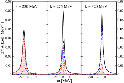
Figure 1: Spectral function for a density of $\rho=0.2\,\mbox{fm}^{-3}$ and a temperature of $T=10\,\mbox{MeV}$ (solid line). Various momenta are considered as indicated in the three panels. $A^{<}$ (dashed line) and $A^{>}$ (dash-dotted line) are also displayed.

Figure 2: Diagrammatic representation of the HF approximation (left) and the energy independent part of the self-consistently dressed self energy (right).

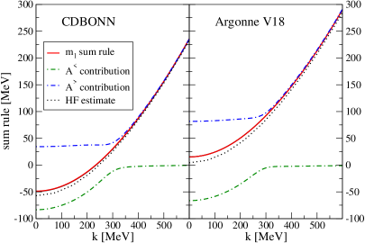
Figure 3: Illustration of the energy weighted sum rule $m_{1}$ (solid lines) for the CDBONN potential (left panel) and the Argonne V18 potential (right panel). Both right hand side and left hand side are displayed, but the sum rule is so well fulfilled that they are on top of each other. The contribution to $m_{1}$ that comes from $A^{>}$ and $A^{<}$ is indicated by the upper and the lower dash-dotted lines, the latter approaching zero rapidly for high momenta. The dotted line is the Hartree-Fock single particle spectrum. Density and temperature are the same as in Fig. 1.

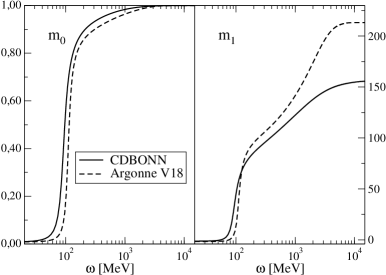
Figure 4: Saturation of the sum rules $m_{0}$ (right panel) and $m_{1}$ (left panel) for the CDBONN potential (solid line) and the Argonne V18 potential (dashed line). The momentum is $k=500\,\mbox{MeV}$. Again, temperature and density are the same as in Fig. 1.

References

- (1) M. Baldo, Nuclear Methods and the Nuclear Equation of State, Int. Rev. of Nucl. Phys, Vol. 9 (World Scientific, Singapore, 1999).
- (2) H. Müther and A. Polls, Prog. Part. Nucl. Phys. 45, 243 (2000).
- (3) M. F. van Batenburg, Ph.D. thesis, University of Utrecht (2001).
- (4) H. Müther, A. Polls and W. H. Dickhoff, Phys. Rev. C51,3040 (1995).
- (5) O. Benhar, A. Fabrocini and S. Fantoni, Nucl. Phys. A 505, 267 (1989).
- (6) A. Ramos, A. Polls and W. H. Dickhoff, Nucl. Phys. A 503, 1 (1989).
- (7) Y. Dewulf, W. H. Dickhoff, D. Van Neck, E. R. Stoddard and M. Waroquier, Phys. Rev. Let. 90, 152501 (2003).
- (8) W. H. Dickhoff and H. Müther, Rep. Prog. Phys. 55, 1947 (1992).
- (9) P. Bożek, Phys. Rev. C 59, 2619 (1999).
- (10) P. Bożek, Phys. Rev. C 65, 054306 (2002).
- (11) T. Frick and H. Müther, Phys. Rev. C 68, 034310 (2003).
- (12) A. Polls, A. Ramos, J. Ventura, S. Amari and W. H. Dickhoff, Phys. Rev. C 49, 3050 (1994).
- (13) W. D. Kraeft, D. Kremp, W. Ebeling and G. Röpke, Quantum Statistics of Charged Particle Systems (Akademie-Verlag, Berlin, 1986).
- (14) L. P. Kadanoff and G. Baym, Quantum Statistical Mechanics (Benjamin, New York, 1962).