Energy averages over regular and chaotic states in the decay out of superdeformed bands

Abstract

We describe the decay out of a superdeformed band using the methods of reaction theory. Assuming that decay-out occurs due to equal coupling (on average) to a sea of equivalent chaotic normally deformed (ND) states, we calculate the average intraband decay intensity and show that it can be written as an “optical” background term plus a fluctuation term, in total analogy with average nuclear cross sections. We also calculate the variance in closed form. We investigate how these objects are modified when the decay to the ND states occurs via an ND doorway and the ND states’ statistical properties are changed from chaotic to regular. We show that the average decay intensity depends on two dimensionless variables in the first case while in the second case, four variables enter the picture.

1 Introduction

The first superdeformed (SD) rotational band to be observed was that identified in the nucleus ${}^{152}_{66}$Dy₈₆ by Twin et al.[1]. A sequence of nineteen $\gamma$-rays of nearly constant spacing was observed which permitted the attribution of the moment of inertia of a symmetric prolate rigid rotor with elliptic axes in the proportion 1:1:2. Since then 320 SD bands have been observed in various mass regions extending from $A$$\sim$20 to $A$$\sim$240[2]. The stability of nuclei at any deformation can be related to the existence of energy gaps between shells of independent particle states. The shell gaps which appear for certain nuclear deformations give origin to non-spherical configurations of special stability[3, 4].

As explained by Lopez-Martens et al.[5], the $\gamma$-spectrum of a compound nucleus whose decay path includes an SD band typically contains $\gamma$-rays which result from four distinct stages:

1. Statistical $\gamma$-rays which populate the SD band after formation of the nucleus under consideration by particle evaporation following a fusion evaporation or fragmentation reaction.

2. Collective $E$2 $\gamma$-rays from decay along the SD band.

3. Statistical $\gamma$-rays from excited normally deformed (ND) configurations.

4. Collective $E$2 $\gamma$-rays from decay along the yrast ND band.

In cases where this kind of decay scheme applies, stages I and III correspond to the cooling of a hot and chaotic system while stages II and IV correspond to the decay of a cold and regular system. Other decay schemes which include SD bands are possible. An SD state may fission or emit particles instead of decaying to the ground state by $\gamma$-emission. Stage II shows the following intensity profile as a function of transition energy, rotational frequency or spin:[6] gradual population at high spin, a plateau at intermediate spin and sudden depopulation at low spin (between 10 and 30 $\hbar$ depending on the mass region).

SD bands by definition are found in the second minimum of the potential energy surface in deformation space (hyperdeformed bands in the third if they can be observed). For a certain interval in spin this minimum coexists with the first minimum where the ND states are found. Between these two minima there is a barrier of typically a few MeV in height. Rotational bands exist in both minima over a large interval in spin. For low spins an ND band is yrast while for higher spins an SD band is yrast. At a certain spin these two bands cross. Decreasing in spin from the crossing point the excitation energy of the SD band relative to the ND band increases due to the different moments of inertia of the two bands. At some moment states in the SD band begin to decay to states in the ND minimum. This transition between stages II and III proceeds by tunneling through the multidimensional barrier in deformation space[7, 8].

In most cases it has not been possible to connect SD bands to the rest of the known decay scheme and consequently only $\gamma$-transition energies, lifetimes and branching rations are known. The reason is the complexity of the ND decay scheme and our incomplete knowledge of it. In just 10% of the 320 bands identified have absolute excitation energies, spins and parities been designated[9, 10, 11].

In the present paper we are interested in stage II of the $\gamma$-intensity. In fact we shall not discuss the feeding[12] of SD bands and restrict ourselves to the decay out. In Section 2 we present analytic formulae for the energy average (including the energy average of the fluctuation contribution) and variance of the intraband decay intensity of a SD band in terms of variables which usefully describe the decay-out [13, 14, 15]. In agreement with Gu and Weidenmüller [14] (GW) we find that average of the total intraband decay intensity can be written as a function of the dimensionless variables $\Gamma^{\downarrow}/\Gamma_{S}$ and $\Gamma_{N}/D$ where $\Gamma^{\downarrow}$ is the spreading width for the mixing of an SD state with ND states of the same spin, $D$ is the mean level spacing of the latter and $\Gamma_{S}$ $(\Gamma_{N})$ are the electromagnetic decay widths of the SD (ND) states. Our formula for the variance of the total intraband decay intensity, in addition to the two dimensionless variables just mentioned, depends on the dimensionless variable $\Gamma_{N}/(\Gamma_{S}+\Gamma^{\downarrow})$.

The results of Section 2 depend on two statistical assumptions. Firstly it is assumed that the states in the ND minimum are chaotic and that their statistical properties can be described by the GOE. Secondly, it is assumed that on average the SD band couples with equal strength to all ND states. However it might be appropriate in some mass regions where the decay out occurs at lower excitation energy to describe the ND states by Poisson statistics. Further, it may be incorrect to assume that all ND states are equivalent. Certain ND states which have a stronger overlap with the SD states may serve as doorways[16] to the remaining ND configurations. In Section 3 a model for which the ND states obey Poisson statistics and for which an SD state couples to a single ND doorway is discussed[17, 18]. It is shown that the addition variables become important.

2 Energy average and variance of the decay intensity

The total intraband decay intensity has the form [17, 14]

$$I=\left(2\pi\Gamma_{S}\right)^{-1}\int_{-\infty}^{\infty}dE|A_{00}(E)|^{2},$$ (1)

where $A_{00}(E)$ is the intraband decay amplitude and $\Gamma_{S}$ is the electromagnetic decay width of SD state $|0\rangle$. The energy average of Eq. (1) may be written as the incoherent sum [15, 19] $\overline{I}=I_{\rm{av}}+\overline{I_{\rm{fl}}}$, where

$$I_{\rm{av}}=\overline{I_{\rm{av}}}=\left(2\pi\Gamma_{S}\right)^{-1}\int_{-\infty}^{\infty}dE\left|\overline{A_{00}(E)}\right|^{2}$$ (2)

and

$$\overline{I_{\rm{fl}}}=\left(2\pi\Gamma_{S}\right)^{-1}\int_{-\infty}^{\infty}dE\overline{\left|A_{00}^{\rm{fl}}(E)\right|^{2}},$$ (3)

where we have written the decay amplitude as $A_{00}=\overline{A_{00}}+A_{00}^{\rm{fl}}$ where $\overline{A_{00}}$ is a background contribution and $A_{00}^{\rm{fl}}$ is the fluctuation on that background. Sargeant et al.[15] took the background to be

$$\overline{A_{00}}=\frac{\Gamma_{S}}{E-E_{0}+i(\Gamma_{S}+\Gamma^{\downarrow})/2}.$$ (4)

Eq. (4) exhibits the structure of an isolated doorway resonance. The doorway $|0\rangle$ has an escape width $\Gamma_{S}$ for decay to the SD state with next lower spin and a spreading width $\Gamma^{\downarrow}=2\pi v^{2}/D$ where $v^{2}$ is the mean square coupling of $|0\rangle$ to the ND states whose level spacing is $D$.

The auto-correlation function of the decay amplitude is given by[15]

$$\overline{A_{00}^{\rm{fl}}(E){A_{00}^{\rm{fl}}(E^{\prime})}^{*}} \approx 2\left(2\pi\Gamma_{N}/D\right)^{-1}(\Gamma^{\downarrow}/\Gamma_{S})^{2}\hskip 5.69054pt{\overline{A_{00}(E)}}^{2}\hskip 5.69054pt\frac{i\Gamma_{N}}{E-E^{\prime}+i\Gamma_{N}}\overline{{A_{00}(E^{\prime})}^{*}}^{2}.$$ (5)

When $E^{\prime}=E$ this reduces to

$$\overline{\left|A_{00}^{\rm{fl}}\right|^{2}}=2\left(2\pi\Gamma_{N}/D\right)^{-1}\frac{{\Gamma_{S}}^{2}{\Gamma^{\downarrow}}^{2}}{\left[(E-E_{0})^{2}+(\Gamma_{S}+\Gamma^{\downarrow})^{2}/4\right]^{2}},$$ (6)

which is the average of the fluctuation contribution to the transition intensity.

The integrals in Eqs. (2) and (3) may be carried out using the calculus of residues. One obtains

$$I_{\rm{av}}^{\rm{GOE}}=(1+\Gamma^{\downarrow}/\Gamma_{S})^{-1},$$ (7)

for the average background contribution and

$$\overline{I_{\rm{fl}}} = 2\left(\pi\Gamma_{N}/D\right)^{-1}\frac{\left(\Gamma^{\downarrow}/\Gamma_{S}\right)^{2}}{\left(1+\Gamma^{\downarrow}/\Gamma_{S}\right)^{3}}=2\left(\pi\Gamma_{N}/D\right)^{-1}I_{\rm{av}}\left(1-I_{\rm{av}}\right)^{2},$$ (8)

for the average fluctuation contribution to the average decay intensity. Eq. (8) for $\overline{I_{\rm{fl}}}$ was compared to the fit formula, obtained by GW,

$$\overline{I_{\rm{fl}}^{\rm{GW}}} = \left[1-0.9139\left(\Gamma_{N}/D\right)^{0.2172}\right]\exp\left\{-\frac{\left[0.4343\ln\left(\frac{\Gamma^{\downarrow}}{\Gamma_{S}}\right)-0.45\left(\frac{\Gamma_{N}}{d}\right)^{-0.1303}\right]^{2}}{\left(\Gamma_{N}/D\right)^{-0.1477}}\right\}.$$

and qualitative agreement of the two formulae found[15]. The dependence of $\overline{I_{\rm{fl}}}$ (and that of $I_{\rm{av}}$) on $\Gamma^{\downarrow}/\Gamma_{S}$ results from the resonant doorway energy dependence of the decay amplitude $\overline{A_{00}(E)}$ [Eq. (4)]. This energy dependence also manifests itself in the average of the fluctuation contribution to the transition intensity $\overline{|A^{\rm{fl}}_{00}(E)|^{2}}$ [Eq. (6)]. GW include precisely the same energy dependence in their calculation by use of an energy dependent transmission coefficient to describe decay to the SD band. This is the reason for our qualitative agreement with GW concerning $\overline{I}$.

A measure of the dispersion of the calculated $I$ is given by the variance $\overline{\left(\Delta I\right)^{2}}=\overline{\left(I-\overline{I}\right)^{2}}$. It was shown[15] that

$$\overline{\left(\Delta I\right)^{2}}={\overline{I_{\rm{fl}}}}^{2}f_{1}\left(\xi\right)+2I_{\rm{av}}\overline{I_{\rm{fl}}}f_{2}\left(\xi\right),$$ (10)

where the variable $\xi$ is defined by

$$\xi\equiv\frac{\Gamma_{S}+\Gamma^{\downarrow}}{\Gamma_{N}}=\frac{\Gamma_{S}}{\Gamma_{N}}(1+\Gamma^{\downarrow}/\Gamma_{S})=\frac{\Gamma_{S}}{D}\frac{D}{\Gamma_{N}}{I_{\rm{av}}}^{-1},$$ (11)

and

$$f_{1}\left(\xi\right)=\frac{1}{\left(1+\xi\right)}+\frac{\xi}{\left(1+\xi\right)^{2}}+\frac{\xi^{2}}{2\left(1+\xi\right)^{3}}\hskip 14.22636pt\mbox{and}\hskip 14.22636ptf_{2}\left(\xi\right)=\frac{1}{2\left(1+\xi\right)}.$$ (12)

Since the variance depends only on $(\Gamma_{S}+\Gamma^{\downarrow})/\Gamma_{N}$ in addition to $\Gamma^{\downarrow}/\Gamma_{S}$ and $\Gamma_{N}/D$, upon fixing the latter two variables the variance may be considered a function of any one of $\Gamma^{\downarrow}/\Gamma_{N}$, $\Gamma_{S}/\Gamma_{N}$, $\Gamma^{\downarrow}/D$ or $\Gamma_{S}/D$ [see Eq. (11)]. Our result for the variance of the decay intensity, $\overline{\left(\Delta I\right)^{2}}$ [Eq. (10)] has a structure reminiscent of Ericson’s expression for the variance of the cross section [20]. In the case compound nucleus scattering, extraction of the correlation width from a measurement of cross section autocorrelation function permits the determination of the density of states of the compound nucleus [21]. In the present case the variance supplies a second “equation” besides that for $\overline{I}$. Both equations are functions of $\Gamma^{\downarrow}$ and $D$, since the electromagnetic widths are measured. Thus both $\Gamma^{\downarrow}$ and $D$ can be unambiguously determined. The derivation in this section is strictly valid only for $\Gamma_{N}/D\gg 1$[15]. However the formulae were found to be qualitatively correct even for $\Gamma_{N}<1$[15].

3 Regularity versus chaos in the ND minimum

Åberg[18] has suggested that an order-chaos transition in the ND states enhances the tunneling probability between the SD and ND wells and consequently that the decay-out of SD bands is an example of “chaos assisted tunneling”. Crucial to the argument[17] is a postulate that the decay-out occurs via an ND doorway state. An ND doorway state can be visualized as being the tail in the ND minimum of the wavefunction of the zero-point vibration in the SD minimum which may be constructed by the Generator Coordinate Method (GCM) of Bonche et al.[22]. Microscopically the vibration is a coherent superposition of 1p-1h states which is damped by the two body residual interaction. Depending on the strength of the residual interaction the 2p-2h states will be regular, chaotic or intermediate between these two limits. Decreasing in spin from the point where the SD and ND bands cross, the excitation energy of the SD band relative to the ND band increases. Near the crossing point the residual interaction is weak, therefore the ND states may be characterized by quantum numbers which are approximately conserved and their energy spectrum exhibits degeneracies. In the language of quantum chaos the ND states are regular and obey Poisson statistics. As the spin decreases the residual interaction grows with the increasing excitation energy, destroying degeneracies and increasing the complexity of the ND states until the regime of quantum chaos is reached as characterized by the GOE. This is a plausible picture of the evolution of the nuclear Hamiltonian with decreasing spin. Given that it is correct, how is the cascade down the superdeformed band modified by an order-chaos transition in the ND minimum?

Åberg[18] constructed a random matrix model for the ND states which interpolates between Poisson and GOE statistics by varying the chaoticity parameter $\lambda$ continuously in the range $0<\lambda\leq 1$. The parameter $\lambda$ which is the determined by the ratio of the variances of the diagonal and off-diagonal random Hamiltonian matrix elements simulates the effect of the residual interaction. The SD state is assumed to lie in middle of the ND spectrum and the doorway is chosen to be an ND state which lies halfway between the SD state and the edge of the ND spectrum. The tunneling probability is given by $T_{\rm{SD}\rightarrow\rm{ND}}=\sum|a^{\prime}_{\mu}|^{2}$ where $a^{\prime}_{\mu}$ is the amplitude of the nuclear wavefunction in ND state $\mu$. The broadening of the distribution of the $a^{\prime}_{\mu}$ by the residual interaction results in an increase in $T_{\rm{SD}\rightarrow\rm{ND}}$ which is denoted “chaos assisted tunneling”. The enhancement in the tunneling probability due to the transition from regularity to chaos is deduced from the ratio of $T_{\rm{SD}\rightarrow\rm{ND}}$ for $\lambda=0.001$ to $T_{\rm{SD}\rightarrow\rm{ND}}$ for $\lambda=0.1$. The value of this ratio is estimated to be $N$ where $N$ is the number of ND states.

Although this idea is also plausible it is not clear what the effect of the change in $T_{\rm{SD}\rightarrow\rm{ND}}$ calculated by Åberg[18] has on the average of the total relative decay intensity of the collective $E$2 electromagnetic transitions of SD bands where the sudden attenuation is experimentally observed. We calculated[17] the background contribution to this quantity for Åberg’s model using the reaction theory methods which were outlined in Section 2 and conclude that the order-chaos transition cannot explain the decay-out.

Instead of Eq. (4) let us now take the background decay amplitude to be[17]

$$\overline{A_{00}}=\frac{\Gamma_{S}}{E-E_{0}+i[\Gamma_{S}+\overline{W}_{00}(E)]/2}.$$ (13)

Following Åberg[18] we assume that $|0\rangle$ only mixes with one ND doorway state $|d\rangle$ whose energy is $E_{d}$. The state $|d\rangle$ is subsequently mixed by the residual interaction with the remaining ND states, $|Q\rangle$, $Q=1,...N$, having the same spin as $|0\rangle$ and $|d\rangle$. The self-energy is then given by

$$\overline{W}_{00}(E)=|V_{0d}|^{2}\sum_{Q=0}^{N}\frac{|c_{d}(Q)|^{2}}{E-E_{Q}+i\Gamma_{N}/2},$$ (14)

where $V_{0d}$ is the interaction energy of $|0\rangle$ and $|d\rangle$ and $c_{d}(Q)$ is the amplitude of $|d\rangle$ in $|Q\rangle$. The $|Q\rangle$ lie in the interval $L=ND$ where $D$ here denotes the mean spacing in energy of the $|Q\rangle$.

Ignoring an energy shift of $|0\rangle$, the background decay intensity becomes

$$I_{\rm{av}}=\frac{\Gamma_{S}}{2\pi}\int_{-\infty}^{\infty}dE\frac{1}{[E-E_{0}]^{2}+[\Gamma_{S}+2\pi|V_{0d}|^{2}S_{d}(E)]^{2}/4},\hskip 11.38109pt$$ (15)

where the doorway strength function is given by

$$S_{d}(E)=\frac{\Gamma_{N}}{2\pi}\sum_{Q=0}^{N}\frac{|c_{d}(Q)|^{2}}{(E-E_{Q})^{2}+\Gamma_{N}^{2}/4}.$$ (16)

In Sargeant et al.[17] the effect of the chaoticity of the ND states on $I_{\rm{av}}$ was investigated by varying the strength of the residual interaction of the $|Q\rangle$ and their interaction with $|d\rangle$, both being assumed to be proportional to the chaoticity parameter $\lambda$. The limiting value $\lambda$=$0$ results in the $|Q\rangle$ having Poisson statistics (regularity) while $\lambda$=$1$ results in their having GOE statistics (chaos). The value of $\lambda$ determines the shape of $S_{d}(E)$ which is precisely the strength function that was previously investigated as a function of $\lambda$[23].

Instead of studying the interpolation between the limits $\lambda$=$0$ and $\lambda$=$1$ by numerically diagonalising random matrices and performing ensemble averages as we did before[23, 17], here we restrict ourselves to the limiting case $\lambda$=$0$. As $\lambda\rightarrow 0$, $c_{d}(Q)\rightarrow\delta_{dQ}$ so that $S_{d}(E)$ reduces to the single Breit-Wigner term,

$$S_{d}^{\rm{Poi}}(E)=\frac{1}{2\pi}\frac{\Gamma_{N}}{(E-E_{d})^{2}+\Gamma_{N}^{2}/4}.$$ (17)

When $\lambda\rightarrow 0$ and $\Gamma_{N}\rightarrow 0$, then $S_{d}(E)\rightarrow\delta(E-E_{d})$. For non-zero $\lambda$, $S_{d}(E)$ broadens with increasing $\lambda$ until when $\lambda=1$ it takes a form, independent of $\Gamma_{N}$, which is well approximated by [23]

$$S_{d}^{\rm{GOE}}(E)=\left\{\begin{array}[]{cc}1,&|E-E_{d}|\leq L/2\\ 0,&|E-E_{d}|>L/2\end{array}\right..$$ (18)

Inserting Eq. (18) into Eq. (15) we find that $I_{\rm{av}}^{\rm{GOE}}=(1+\Gamma^{\downarrow}/\Gamma_{S})^{-1}$ as long as $\Gamma_{S}+\Gamma^{\downarrow}\ll L$, in agreement with Eq. (7) of Section 2. Gu et al. discuss the strength function further for $L$ finite[24] and $L$ infinite[25].

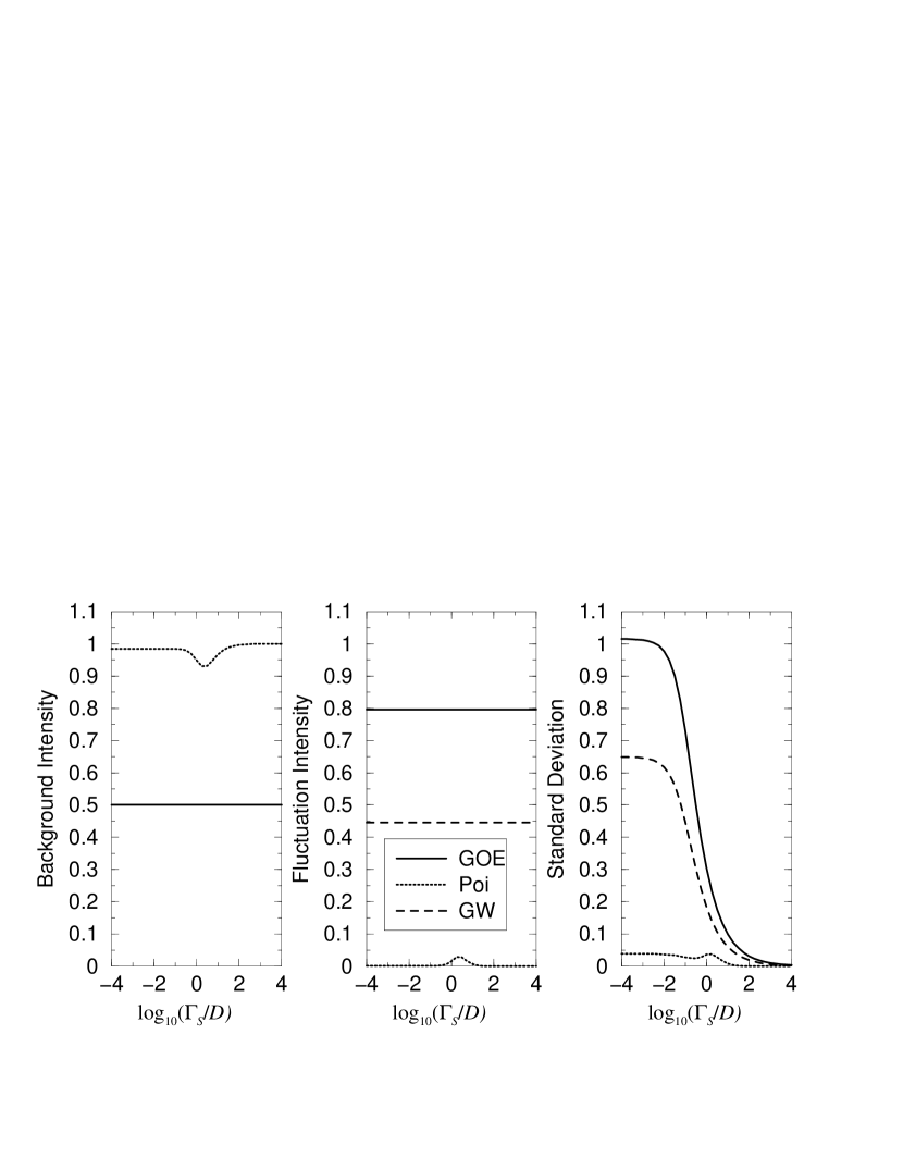
Figure 1: The left graph shows the average background decay intensity versus $\log_{10}(\Gamma_{S}/D)$ [The solid line was calculated using Eq. (7) and the dotted line using Eq. (19)]. The middle graph shows the fluctuation contribution to the average decay intensity versus $\log_{10}(\Gamma_{S}/D)$ [The solid line was calculated using Eq. (8) with Eq. (7) and the dotted line using Eq. (8) with Eq. (19). The dashed line was calculated using Eq. (LABEL:gufit)]. The right graph shows the standard deviation of the decay intensity (=$\sqrt{\overline{\left(\Delta I\right)^{2}}}$) versus $\log_{10}(\Gamma_{S}/D)$ [The solid line was calculated using Eq. (10) with Eqs. (8) and (7) and the dotted line using Eq. (10) with Eqs. (8) and (19). The dashed line was calculated using Eq. (10) with Eq. (LABEL:gufit)]. The following numerical values were used to plot the graphs: $\Gamma^{\downarrow}/\Gamma_{S}=1$, $\Gamma_{N}/D=0.1$ and $\Delta/D$=1.

Eq. (15) for $I_{\rm{av}}$ with $S_{d}=S_{d}^{\rm{Poi}}$ depends on four parameters: $\Gamma_{S}$, $|V_{0d}|^{2}$, $\Gamma_{N}$ and the distance in energy separating $|d\rangle$ from $|0\rangle$, $\Delta=E_{d}-E_{0}$. It is useful to introduce a spreading width now defined to be $\Gamma^{\downarrow}=2\pi|V_{0d}|^{2}/D$. Inserting Eq. (17) into Eq. (15) yields our result for $I_{\rm{av}}$ in the Poisson limit: upon making the change of integration variable $x=(E-E_{0})/D$ this takes the form

$$I_{\rm{av}}^{\rm{Poi}}=\frac{\Gamma_{S}/D}{2\pi}\int_{-\infty}^{\infty}dx\frac{1}{x^{2}+\left(\Gamma_{S}/D\right)^{2}\left[1+\frac{\Gamma^{\downarrow}}{\Gamma_{S}}\frac{1}{2\pi}\frac{\Gamma_{N}/D}{[x-\Delta/D]^{2}+(\Gamma_{N}/D)^{2}/4}\right]^{2}/4}.$$ (19)

It is seen from Eq. (19) that, in addition to $\Gamma^{\downarrow}/\Gamma_{S}$, $I_{\rm{av}}^{\rm{Poi}}$ is a function of a further three dimensionless variables: $\Gamma_{N}/D$, $\Gamma_{S}/D$ and $\Delta/D$.

The introduction of the ND doorway is analogous to including another class of complexity in multistep compound preequilibrium reactions[26, 27]. Calculation of the fluctuation contribution to the average decay intensity and the variance in the presence of an ND doorway is beyond the scope of this paper. However, since Eq. (8) for the fluctuation contribution and Eq. (10) for the variance are expressible in terms of the background contribution, $I_{\rm{av}}$, one can obtain add hoc estimates by simply substituting Eq. (19) into Eqs. (8) and (10) (see Figure 1). A rigorous calculation of the fluctuation contribution and variance when the ND states obey Poisson statistics may be possible using the averaging method of Gorin[28].

The most important conclusion to be drawn from Figure 1 is that a measurement of the variance (standard deviation) of the decay intensity determines the density of ND states $\rho=1/D$. For comparison we have also calculated the standard deviation by inserting the GW fit formula [Eq. (LABEL:gufit)] into our formula for the variance [Eq. (10)].

Eq. (19) is formally identical to the branching ratio, $F_{S}$, calculated by Stafford and Barrett[29] (SB). They model the decay-out by allowing a single SD state to mix with a single ND state. SB and Dzyublik and Utyuzh[30] who develop the method of SB further address the lack of knowledge of $\Delta$ by averaging over $\Delta$ assuming a uniform distribution[31]. Cardamone et al.[32] on the other hand assume a Wigner distribution, $P_{\rm{GOE}}(\Delta)=\pi\Delta/2\exp(-\pi\Delta^{2}/4)$. The preceding discussion suggests that a Poisson distribution $P_{\rm{Poi}}(\Delta)=\exp(-\Delta)$ is more appropriate.

An Addendum to Sargeant et al.[17] is in preparation, where we shall discuss the question of whether the order-chaos transition can explain the decay-out when $\Delta$ is non-zero[33].

References

- [1] P. J. Twin, B. M. Nyakó, A. H. Nelson et al., Phys. Rev. Lett. 57 (1986) 811.
- [2] B. Singh, R. Zywina and R. B. Firestone, Nucl. Data Sheets 97 (2002) 241.
- [3] S. G. Nilsson and I. Ragnarsson, Shapes and Shells in Nuclear Structure (Cambr., 1995).
- [4] R. Wadsworth and P. J. Nolan, Rep. Prog. Phys. 65 (2002) 1079.
- [5] A. Lopez-Martens, F. Hannachi, A. Korichi et al., Acta Phys. Pol. B 34 (2003) 2195.
- [6] A. Lopez-Martens, T. Døssing, T. L. Khoo et al., Phys. Scr. T88 (2000) 28.
- [7] Y. R. Shimizu, F. Barranco, R. A. Broglia et al., Phys. Lett. B 274 (1992) 253.
- [8] K. Yoshida, M. Matsuo and Y. R. Shimizu, Nucl. Phys. A696 (2001) 85.
- [9] T. Lauritsen, M. P. Carpenter, T. Døssing et al., Phys. Rev. Lett. 88 (2002) 042501.
- [10] A. N. Wilson, G. D. Dracoulis, A. P. Byrne et al., Phys. Rev. Lett. 90 (2003) 142501.
- [11] E. S. Paul, S. A. Forbes, J. Gizon et al., Nucl. Phys. A690 (2001) 341.
- [12] T. L. Khoo, T. Lauritsen, I. Ahmad et al., Nucl. Phys. A557 (1993) 83.
- [13] R. Krucken, A. Dewald, P. von Brentano et al., Phys. Rev. C 64 (2001) 064316.
- [14] J.-z. Gu and H. A. Weidenmüller, Nucl. Phys. A660 (1999) 197.
- [15] A. J. Sargeant, M. S. Hussein, M. P. Pato et al., Phys. Rev. C 66 (2002) 064301.
- [16] C. Andreoiu, T. Døssing, C. Fahlander et al., Phys. Rev. Lett. 91 (2003) 232502.
- [17] A. J. Sargeant, M. S. Hussein, M. P. Pato et al., Phys. Rev. C 65 (2002) 024302.
- [18] S. Åberg, Phys. Rev. Lett. 82 (1999) 299.
- [19] M. Kawai, A. K. Kerman and K. W. McVoy, Ann. Phys. 75 (1973) 156.
- [20] T. Ericson, Ann. Phys. 23 (1963) 390.
- [21] T. Ericson and T. Mayer-Kuckuk, Annu. Rev. Nucl. Sci. 16 (1966) 183.
- [22] P. Bonche, J. Dobaczewski, H. Flocard et al., Nucl. Phys. A519 (1990) 509.
- [23] A. J. Sargeant, M. S. Hussein, M. P. Pato et al., Phys. Rev. C 61 (2000) 011302.
- [24] J.-z. Gu, L. Gao and B. Hu, Phys. Rev. C 66 (2002) 054312.
- [25] J.-z. Gu, L. Gao and B. Hu, Phys. Rev. E 66 (2002) 026208.
- [26] H. Nishioka, J. J. M. Verbaarschot and H. A. Weidenmüller, Ann. Phys. 172 (1986) 67.
- [27] W. A. Friedman, M. S. Hussein, K. W. McVoy et al., Phys. Rep 77 (1981) 47.
- [28] T. Gorin, J. Phys. A 32 (1999) 2315.
- [29] C. A. Stafford and B. R. Barrett, Phys. Rev. C60 (1999) 051305.
- [30] A. Y. Dzyublik and V. V. Utyuzh, Phys. Rev. C 68 (2003) 24311.
- [31] E. Vigezzi, R. A. Broglia and T. Døssing, Nucl. Phys. A520 (1990) 179c.
- [32] D. M. Cardamone, C. A. Stafford and B. R. Barrett, Phys. Rev. Lett. 91 (2003) 102502.
- [33] S. Åberg, Phys. Rev. C 68 (2003) 069801.