A computationally tractable version of the collective model

Abstract

A computationally tractable version of the Bohr-Mottelson collective model is presented which makes it possible to diagonalize realistic collective models and obtain convergent results in relatively small appropriately chosen subspaces of the collective model Hilbert space. Special features of the proposed model is that it makes use of the beta wave functions given analytically by the softened-beta version of the Wilets-Jean model, proposed by Elliott et al., and a simple algorithm for computing SO(5) $\supset$ SO(3) spherical harmonics. The latter has much in common with the methods of Chacon, Moshinsky, and Sharp but is conceptually and computationally simpler. Results are presented for collective models ranging from the sherical vibrator to the Wilets-Jean and axially symmetric rotor-vibrator models.

I Introduction

This paper presents a computationally tractable version of the standard Bohr-Mottelson (BM) collective model BM ; BMbook ; Rowebook . The need for such a version of the model arises because the expansion of rotational wave functions in a spherical vibrational basis is so slowly convergent that the diagonalization of a general coupled-rotor-vibrator collective model Hamiltonian in this basis is virtually impossible. The proposed method constructs a basis for the collective model in which beta wave functions, centred about a non-zero equilibrium value, are given analytically following the methods of Elliott et al. EEP86 and ref. RB98 , and new methods are developed for computing the complementary rotational and gamma wave functions. The motivation for this development is to be seen in the context of a sequence of steps from a phenomenological model description of nuclear collective structure to a microscopic interpretation of what it means. I follow the strategy of giving a phenomenological collective model a microscopic foundation by first formulating it in algebraic terms and subsequently constructing representations of its algebraic expression on a microscopic shell model Hilbert space.

Early advances in the shell model theory of collectivity came with the identification of seniority and symplectic symmetry with pairing Flowers ; Kerman ; Talmi and su(3) with rotations Elliott . An early description of the use of symmetry in nuclear structure was provided by Parikh Parikh .

Algebraic methods have subsequently had an enormous influence on collective model theory (cf. Rev for a review). Two influential developments have been: the Frankfurt version of the collective model (Greiner ; Hess ) and the Interacting Boson Model (IBM) IBM . The Frankfurt methods were developed to give solutions to the collective model in the intermediate region between the analytically solvable vibrational and rotational limits. They made major use of the algebraic structures associated with the five-dimensional harmonic oscillator. The IBM achieved a reduction of the Frankfurt program to a finite-dimensional space by compactifying the algebraic structure of the collective model to the U(6) symmetry group of the six-dimensional harmonic oscillator and restricting consideration to single (finite-dimensional) U(6) irreps. The IBM has three exactly solvable limits, corresponding to similar limits of the BM model.

Major developments towards the goal of formulating a microscopic (shell model) theory of collective states have also followed the algebraic approach (a historical survey was provided in the review article of ref. EarlyRev ). The latter developments were based on the symplectic model RosRow .

The symplectic model and its several variations have not been applied widely to fit detailed nuclear data because that was not their purpose (cf. refs. BR2000 ; CRKB for some recent applications). Their purpose was to obtain a fundamental explanation of nuclear collective dynamics and the way it emerges from interacting nucleons. Thus, even if one were to succeed in formulating a completely satisfactory theory of nuclear collective dynamics, it would hardly be a simple theory. Nor would it serve the purpose of every-day analysis of nuclear data. For this purpose, one continues to need simple phenomenological models, albeit preferably ones with a microscopic foundation. With this concern in mind, we revisit the BM collective model with the benefit of insights acquired from the Frankfurt model, the IBM, and the symplectic model.

II The standard solvable limits of the collective model

The classic BM collective model shares a Hilbert space with the five-dimensional harmonic oscillator. Indeed, in its harmonic vibrational limit, its spectrum and eigenstates are precisely those of the five-dimensional harmonic oscillator. Thus, it has rich algebraic, geometrical, and analytical structures all which are exploited in this paper. It has a spectrum generating algebra given by the semi-direct sum Lie algebra [HW(5)]u(5) and a corresponding dynamical group [HW(5)]U(5). The Lie algebra [hw(5)]u(5) is spanned by five $(L=2)$ pairs of $d$-boson (phonon) operators $\{d^{\nu},d^{\dagger}_{\nu};\nu=0,\pm 1,\pm 2\}$ and the infinitesimal generators $\{d^{\dagger}_{\mu}d^{\nu}\}$ of U(5), where the $d$-bosons satisfy the commutation relations $[d^{\mu},d^{\dagger}_{\nu}]=\delta_{\mu\nu}$.

The collective model has three well-known algebraically solvable limits: the harmonic vibrator model, the Wilets-Jean (gamma-soft) model WJ , and the axially-symmetric rigid-rotor model. These submodels are associated with dynamical subgroup chains corresponding to different paths through the set of groups

$$\begin{array}[]{ccccccc}{\rm[HW(5)]U(5)}&\supset&{\rm[R^{5}]SO(5)}&\supset&{\rm[R^{5}]SO(3)}\\ \cup&&\cup&&\cup\\ {\rm U(5)}&\supset&{\rm SO(5)}&\supset&{\rm SO(3)}&&\end{array}$$ (1)

starting with [HW(5)]U(5) and ending with SO(3), where R⁵ is the group with Lie algebra spanned by the quadrupole moments

$$\Big{\{}\hat{Q}_{\nu}={1\over\sqrt{2}}\,(d^{\dagger}_{\nu}+d_{\nu})\,,\nu=0,\pm 1,\pm 2\Big{\}}$$ (2)

with $d_{\nu}=(-1)^{\nu}d^{-\nu}$. Thus,

$${\rm[HW(5)]U(5)}\supset{\rm U(5)}\supset{\rm SO(5)}\supset{\rm SO(3)}$$ (3)

is a dynamical subgroup chain for the harmonic vibrator model,

$${\rm[HW(5)]U(5)}\supset{\rm[R^{5}]SO(5)}\supset{\rm SO(5)}\supset{\rm SO(3)}$$ (4)

is a dynamical subgroup chain for the Wilets-Jean (beta-rigid, gamma-soft) model, and

$${\rm[HW(5)]U(5)}\supset{\rm[R^{5}]SO(5)}\supset{\rm[R^{5}]SO(3)}\supset{\rm SO(3)}$$ (5)

is a dynamical chain for the rigid-rotor (beta- and gamma-rigid) model. The above subgroup chains are discussed in more detail, for example, in ref. Rev .

The solution of more general collective model Hamiltonians has been tackled, for example, by Hess et al. Hess in the U(5) $\supset$ SO(5) $\supset$ SO(3) basis for the collective model Hilbert space of Chacon, Moshinsky and Sharp CMS . This approach has been very influential and has applications to the IBM in which the same U(5) and SO(5) $\supset$ SO(3) groups also appear. Its limitation is that it is impractical for the description of collective model states of large deformation which converge extremely slowly in a spherical U(5) basis.

III An alternative basis for the collective model

Moving between the above solvable limits of the collective model is complicated by the ‘rigidity’ of two of the limits. Both the rigid-rotor model and the beta-rigid gamma-soft (Wilets-Jean) model have delta function components to their wave functions and, as a consequence, they are not realizable in the Hilbert space of the vibrator limit except as limits of sequences of normalizable wave functions. This limitation expresses the fact that rigidly-defined intrinsic quadrupole moments are unphysical and incompatible with quantum mechanics (as well as relativity theory). I therefore consider an alternative basis for the diagonalization of collective model Hamiltonians and show that it can lead to convergent solutions for a wide range of collective model Hamiltonians.

An important feature of the collective model is that its coordinates separate into orthogonal subsets in much the same way as those of a single particle in three-dimensional space separate into radial and spherical coordinates. Associated with this observation is the fact that the Hilbert space of the collective model is a direct sum

$$\mathbb{H}^{{\rm CM}}=\bigoplus_{v}\mathbb{H}_{v}=\bigoplus_{v}\,\mathbb{H}^{{\rm SU(1,1)}}_{v}\otimes\mathbb{H}^{{\rm SO(5)}}_{v}\,,$$ (6)

of Hilbert spaces labeled by a seniority quantum number $v$, which each carry an irrep of a direct product group SU(1,1)$\times$SO(5), where SU(1,1) is the group of scale transformations of the beta (radial) coordinate, defined by $\beta^{2}=Q\cdot Q$, and SO(5) is the five-dimensional rotation group. As a result of this separation of variables, SO(5)-invariant collective model Hamiltonians can be diagonalized with just the Lie algebra of SU(1,1) as spectrum generating algebra.

Thus, for example, the collective model has two other exactly solvable submodels given by simply adding a $1/\beta^{2}$ term to either the five-dimensional harmonic oscillator Hamiltonian EEP86 or to the five-dimensional analog of the Coulomb Hamiltonian FV . Such models are known in three dimensions as the Davidson Davidson and Kratzer models Krat . Algebraic solutions of three-dimensional central-force problems, have been studied widely in terms of the algebra of the direct product group SU(1,1)$\times$SO(3) (reviewed in ref. CP ; an historic account is given in Wybourne’s book Wyb and an overview of the basic methods in ref. CW ). The natural extension of the algebraic treatment to five-dimensional space with dynamical group SU(1,1)$\times$SO(5) is straightforward RB98 ; Rev . The fact that solvable central force problems remain solvable on addition of a $1/r^{2}$ term to the Hamiltonian follows from the observation that the commutation relations of the SU(1,1) spectrum generating algebras are unchanged, by the substitution $\nabla^{2}\to\nabla^{2}+k/r^{2}$. This result holds in higher-dimensional spaces.

Following the standard methods for three-dimensional central-force problems , the spectrum and wave functions for the five-dimensional harmonic oscillator

$$\hat{H}=-{\hbar^{2}\over 2B}\nabla^{2}+{1\over 2}B\omega^{2}\beta^{2},$$ (7)

are given by

$$E_{nv}=(2n+\lambda_{v})\hbar\omega,\quad n=0,1,2,\dots\quad v=0,1,2,\dots$$ (8)

and

$$\Psi_{nv\sigma}(\beta,\omega)=\sqrt{2n!\over\Gamma(n+\lambda_{v})b^{5}}\ \Big{(}{\beta\over b}\Big{)}^{\lambda_{v}-{5\over 2}}\exp\Big{(}-{\beta^{2}\over 2b^{2}}\Big{)}\,L^{(\lambda_{v}-1)}_{n}\Big{(}{\beta^{2}\over b^{2}}\Big{)}\,\mathcal{Y}_{v\sigma}(\omega),$$ (9)

where $\mathcal{Y}_{v\sigma}$ is an SO(5) spherical harmonic for an SO(5) irrep of seniority $v$, $L_{n}^{(\lambda_{v}-1)}$ is an associated Laguerre polynomal, and $\lambda_{v}=v+5/2$, $b=\sqrt{\hbar/B\omega}$.

The above (standard) results are obtained by use of the SU(1,1) Lie algebra spanned by the operators

$$\hat{Z}_{1}=-\nabla^{2},\quad\hat{Z}_{2}=\beta^{2},\quad\hat{Z}_{3}=-i(q\cdot\nabla+\textstyle{5\over 2})\,.$$ (10)

Because the commutation relations of these operator are unchanged if $\hat{Z}_{1}$ is replaced by

$$\hat{Z}_{1}^{\prime}=-\nabla^{2}+{\beta_{0}^{4}\over\beta^{2}},$$ (11)

it follows RB98 that the harmonic vibrational limit of the collective model extends immediately to a model with beta-vibrational Hamiltonian

$$\hat{H}(\beta_{0})={\hbar^{2}\over 2B}\Big{(}-\nabla^{2}+{\beta_{0}^{4}\over\beta^{2}}\Big{)}+{1\over 2}B\omega^{2}\beta^{2},$$ (12)

The only change in the results of the harmonic vibrational limit for the energies $\{E_{nv}\}$ and wave functions $\{\Psi_{nv\sigma}\}$ is that the relationship $\lambda_{v}=v+5/2$ is generalized to

$$\lambda_{v}=1+\sqrt{(v+\textstyle{3\over 2})^{2}+\beta_{0}^{4}}\,.$$ (13)

This is because the replacement $\hat{Z}_{1}\to\hat{Z}_{1}^{\prime}$ in the SU(1,1) Lie algebra results RB98 in a modification of the value of the SU(1,1) Casimir invariant from the value $\lambda_{v}(\lambda_{v}-2)=v(v+3)+{5\over 4}$ to the value

$$\lambda_{v}(\lambda_{v}-2)=v(v+3)+\textstyle{5\over 4}+\beta_{0}^{4}\,.$$ (14)

The five-dimensional Kratzer model FV is handled in a similar way as shown in the Appendix.

With explicit wave functions, it is a simple matter to compute observable properties of the model states. For example, the matrix elements of an electric quadrupole operator of the form

$$\hat{Q}_{M}=Z\beta\,\hat{q}_{M}$$ (15)

with $\hat{q}_{M}$ taking the values

$$q_{M}=\cos\gamma\mathcal{D}^{2}_{0,M}(\Omega)+\frac{1}{\sqrt{2}}\sin\gamma\left(\mathcal{D}^{2}_{2,M}(\Omega)+\mathcal{D}^{2}_{-2,M}(\Omega)\right)\,,$$ (16)

factor into products of a matrix element of $\hat{\beta}$ between associated Laguerre polynomials and a matrix element of a $v\!=\!1$ SO(5) spherical harmonic. Thus, the latter matrix elements are given by elementary SO(5) Clebsch-Gordan coefficients as shown explicitly below.

The properties of a sequence of collective models with Hamiltonian $\hat{H}(\beta_{0})$ and with $\beta_{0}$ ranging from zero to a large value are discussed in the following section. It is seen there that the above model provides a sequence of analytically solvable solutions which progress from the harmonic vibrational ${\rm[HW(5)]U(5)}\supset{\rm U(5)}$ limit to the asymptotic Wilets-Jean ${\rm[HW(5)]U(5)}\supset{\rm[R^{5}]SO(5)}$ limit.

Subsequent sections demonstrate that the basis of eqn. (9), which reduces an ${\rm SU(1,1)}\times{\rm SO(5)}\supset{\rm SO(3)}$ dynamical subgroup chain, provides a much more rapidly convergent basis for the expansion of the eigenfunctions of an arbitrary collective model than does a basis that reduces the chain ${\rm U(5)}\supset{\rm SO(5)}\supset{\rm SO(3)}$. For a collective model Hamiltonian that is SO(5)-invariant, the eigenfunctions and spectrum are readily computed using just the Lie algebra of SU(1,1) as a spectrum generating algebra. Convergence is then optimized by selecting a value of $\beta_{0}$ at the minimum of the $\beta$ potential of interest.

For a general collective Hamiltonian, in which both the SU(1,1) and SO(5) degrees are active, expressions are needed for the SO(5) spherical harmonics. They can be constructed by the methods of Chacon et al. CMS . However, I follow a simpler construction based on the observation that the SO(5) spherical harmonics are an orthonormal basis for the Hilbert space $\mathcal{L}^{2}(S_{4})$ of square integrable functions on the four-sphere $S_{4}$ with respect to the usual volume element BM given, in standard $(\gamma,\theta,\varphi)$ coordinates, by

$${\rm d}v=\sin 3\gamma\,{\rm d}\gamma\,{\rm d}\Omega,$$ (17)

where d$\Omega=\sin\theta\,{\rm d}\theta\,{\rm d}\varphi$. A non-orthonormal basis for $\mathcal{L}^{2}(S_{4})$ is simply constructed as shown in sect. V.2. This basis is then Gramm-Schmidt orthogonalized to give the SO(5) spherical harmonics. This method will be deetailed and used to compute a subset of SO(5) Clebsch-Gordan coefficients in a following paper RTR . Thus, the facility to diagonalize any Hamiltonian on the collective model Hilbert space (6) and to compute, for example, $B$(E2) transition rates between its eigenstates, is limited only by the computational power available. An illustrative calculation of the spectrum and E2 transitions for an axially symmetric rotor-vibrator model is given in sect. VII.

IV Results for the basic SO(5)-invariant model

Figure 1 shows the potential energy function

$$V_{\beta_{0}}(\beta)=\frac{\hbar\omega}{2b^{2}}\left(\beta^{2}+\frac{\beta_{0}^{4}}{\beta^{2}}\right)$$ (18)

of the Hamiltonian (12) for $\beta_{0}=0$ and 8 together with the corresponding ground-state $\beta$ wave functions.

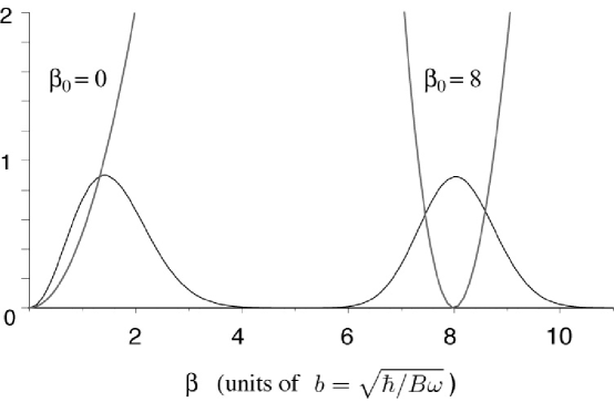
Figure 1: The potential energy components of the Hamiltonian (12) for $\beta_{0}=0$ and 8 together with the corresponding beta wave functions multiplied by $\beta^{2}$. The potential is given in units of $\hbar\omega$.

The ratio of the $\beta$-width to the mean value of $\beta$, given for these wave functions, by $b/\beta_{0}$ is proportional to $1/\beta_{0}\sqrt{\omega}$. Thus, as $\beta_{0}\sqrt{\omega}$ becomes large, the wave functions approach the Wilets-Jean rigid-beta limit.

The energy-level spectrum, given by eqns. (8) and (13) is shown as a function of $\beta$ in fig. 2 for a range of values of the deformation parameter $\beta_{0}$.

Figure 2: Energies of the five-dimensional Davidson model as a function of $\beta_{0}$.

Fig. 2 shows that as $\beta_{0}\sqrt{\omega}\to\infty$ (the Wilets-Jean limit) the energy levels asymptotically approach a harmonic oscillator sequence with the states of each asymptotic level comprising an infinite number of states. Low energy levels for specific values of $\beta_{0}$ are shown in more detail together with $B$(E2) transition rates in figs. 3 and 4.

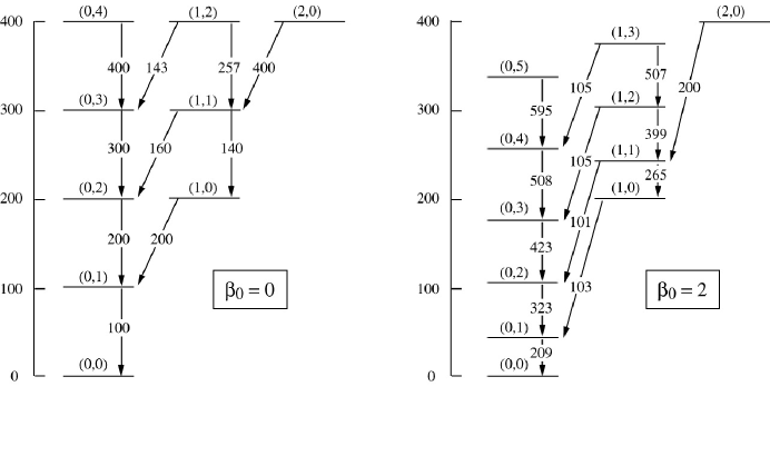
Figure 3: Energy-levels and $B$(E2) transition rates for the Hamiltonian (12) with $\beta_{0}=0$ and 2. Energy levels are labeled by their SU(1,1)$\times$SO(5) quantum numbers $(n,v)$. Energies and $B$(E2) transition rates are given in units such that the one-phonon $L=2$ excited (0,1) state has an excitation energy of 100 units and its $B$(E2) transition rate to the ground state is also 100 units in the U(5) $(\beta_{0}=0)$ limit.

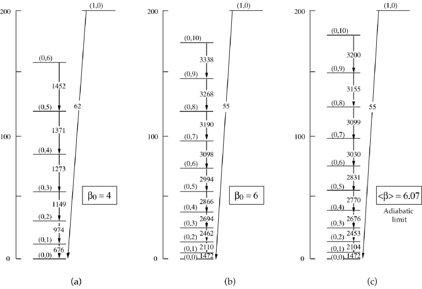
Figure 4: Energy-levels and $B$(E2) transition rates for the Hamiltonian (12) with $\beta_{0}=4$ and 6 in units defined in the caption to fig. 3. For comparison, (c) is the spectrum obtained by a simple adiabatic approximation with $<\hat{\beta}>=6.07$ as described in the text.

$B$(E2) transition rates are computed as follows. Let $\{|nv\sigma\rangle\}$ denote the basis states corresponding to the wave functions of eqn. (9) with $\lambda_{v}$ related to $v$ by eqn. (13). The $B$(E2) transition rate between two SO(5) levels is then defined in the standard way for the quadrupole operator $\hat{Q}$ by summing the squared matrix elements of $\hat{Q}$ over the states of the final level and averaging over initial states. Thus

$$B({\rm E}2;n_{i}v_{i}\to n_{f}v_{f}) = \sum_{\sigma_{i}\sigma_{f}M}\frac{1}{d(v_{i})}|\langle n_{f}v_{f}\sigma_{f}|\hat{Q}_{M}|n_{i}v_{i}\sigma_{i}\rangle|^{2}$$ (19)

$$= \frac{d(v_{f})}{d(v_{i})}|\langle n_{f}v_{f}|||\hat{Q}|||n_{i}v_{i}\rangle|^{2}$$

$$= |\langle n_{i}v_{i}|||\hat{Q}|||n_{f}v_{f}\rangle|^{2},$$

where $d(v)$ is the dimension of the SO(5) irrep of seniority $v$ and $\langle n_{f}v_{f}|||\hat{Q}|||n_{i}v_{i}\rangle$ is an SO(5)-reduced matrix element of the $v=1$ quadrupole tensor. Since the wave functions for the states $\{|nv\sigma\rangle\}$ are products of $\beta$ wave functions and spherical harmonics, the matrix elements of the $\hat{Q}_{M}=Z\hat{\beta}\hat{q}_{M}$ operators of eqn. (15) factor and are given by

$$\langle n_{i}v_{i}|||\hat{Q}|||n_{f}v_{f}\rangle=Z\langle n_{i}v_{i}|\hat{\beta}|n_{f}v_{f}\rangle\langle v_{i}|||\hat{q}|||v_{f}\rangle,$$ (20)

with obvious notation. The $\hat{\beta}$ matrix element is readily evaluated for any value of $\beta_{0}$ while the $\hat{q}$ matrix element is independent of $\beta_{0}$ and can be evaluated in the U(5) ($\beta_{0}=0$) limit.

In the U(5) limit, the $\hat{Q}_{M}$ operator can be expressed in terms of $L=2$ harmonic-oscillator raising and lowering operators

$$\hat{Q}_{M}=Z\frac{d^{\dagger}_{M}+d_{M}}{\sqrt{2}}.$$ (21)

It follows that $\langle 0v|||\hat{Q}|||0v\rangle=0$ and

$$\langle 0,v+1|||\hat{Q}|||0v\rangle=Z\sqrt{(v+1)/2}\ .$$ (22)

Therefore, since the $\beta$ integral gives $\langle 0,v+1|\hat{\beta}|0v\rangle=\sqrt{(2v+5)/2}$, we infer that

$$\langle v+1|||\hat{q}|||v\rangle=\displaystyle\sqrt{\frac{v+1}{2v+5}},$$ (23)

$$\langle v|||\hat{q}|||v+1\rangle=(-1)^{\phi}\displaystyle\sqrt{\frac{v+1}{2v+5}\cdot\frac{d(v+1)}{d(v)}},$$ (24)

where the phase factor $(-1)^{\phi}$ depends on a choice of phase convention. Thus, for arbitrary $\beta_{0}$,

$$B({\rm E}2;n^{\prime}v\to n,v-1)=\displaystyle\frac{Z^{2}v}{2v+3}\langle n^{\prime}v|\hat{\beta}|n,v-1\rangle^{2},$$ (25)

$$B({\rm E}2;n^{\prime}v\to n,v+1)=\displaystyle\frac{Z^{2}(v+1)d(v+1)}{(2v+5)d(v)}\langle n^{\prime}v|\hat{\beta}|n,v+1\rangle^{2}.$$ (26)

It is also follows from the identity $\langle 0v|||\hat{Q}|||0v\rangle=0$ that all quadrupole moments are zero in this model as expected for a gamma-soft model. For the present calculations, $Z^{2}$ was given the value $Z^{2}=200$ so that $B({\rm E}2;2_{1}\to 0_{1})=100$ in the U(5) ($\chi=0$) limit.

It is seen from the figures that, as the value of $\beta_{0}$ is increased, excited beta-vibrational bands separate and increase in energy. In the Wilets-Jean limit, in which $\beta_{0}\sqrt{\omega}\to\infty$, the ratio of the beta-vibrational energy to the lowest rotational excitation energy diverges. As this limit is approached, a simple adiabatic approximation gives increasingly good approximate solution to the results of the Hamiltonian (12) as illustrated by comparison of figs. 4(b) and 4(c).

The adiabatic approximation follows by expanding the expression for the energy (8) with $\lambda_{v}$ given by eqn. (13), for large values of $\beta_{0}$,

$$E_{nv}=\left[2n+\frac{1}{2\beta_{0}^{2}}v(v+3)\right]\hbar\omega+0\left(\frac{1}{\beta_{0}^{4}}\right)+{\rm const.},$$ (27)

and neglecting terms of order $1/\beta_{0}^{4}$ and higher. This approximation corresponds to neglecting the centrifugal coupling between the rotational and beta-vibrational degrees of freedom. Perturbation theory shows that this approximation is good so long as the rotational energy $v(v+3)/2\beta_{0}^{2}$, for the gamma-soft rotor, is small in comparison with the beta-vibrational energy $\hbar\omega$.

The effective decoupling of the beta-vibrational and rotational degrees of freedom in the adiabatic limit, is evidenced by the independence of the beta wave function on the seniority quantum number $v$ in this limit. A comparison is made between the $v=0$, 5, and 10 beta wave functions in fig. 5 for $\beta_{0}=4$, 6, and 8. It is seen that centrifugal stretching is substantial for $\beta_{0}=4$ but negligible for $\beta_{0}\approx 8$ and $v\lesssim 10$

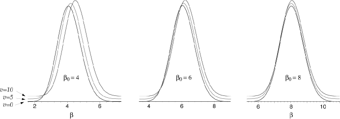
Figure 5: Comparison of the beta components of the model wave functions for $\beta_{0}=4,6,8$ and for $v=0$, 5, and 10. It is seen that the wave functions are shifted to higher values of $\beta$ with increasing $v$ due to centrifugal stretching for small values of $\beta_{0}$ but that as $\beta_{0}\sqrt{\omega}\to\infty$, the adiabatic limit is approached in which this shifting becomes more and more negligible for finite values of $v$.

V More general collective model Hamiltonians

An extension of the above model to admit gamma as well as deformed-beta equilibrium shapes, is given, for example, by adding a gamma-dependent potential to the Hamiltonian (12);

$$\hat{H}={\hbar^{2}\over 2B}\Big{(}-\nabla^{2}+{\beta_{0}^{4}\over\beta^{2}}\Big{)}+{1\over 2}B\omega^{2}\beta^{2}+\hat{V}\,.$$ (28)

To illustrate, I consider the potential

$$V(\gamma)=-\chi\cos 3\gamma$$ (29)

which has an axially symmetric minimum. This potential produces a very tractable model because, to within a constant, $\cos 3\gamma$ is the SO(5) $v=3,L=0$ spherical harmonic. An even simpler model is obtained by assuming a value of $\beta_{0}\sqrt{\omega}$ for which the $\beta$ and SO(5) degrees of freedom are adiabatically decoupled. The latter choice is not necessary but simplifies the calculations considerably.

V.1 The adiabatic map

For each value of the $\beta$ quantum number $n$, the SO(5) quantum number $v$ runs over the complete set of nonnegative integers $v=0$, 1, 2, $\dots$. Moreover, just as the set of SO(3) spherical harmonics $\{Y_{LM}\}$ spans the Hilbert space $\mathcal{L}^{2}(S_{2})$ of square integrable functions on the two-sphere, so the set of SO(5) spherical harmonics $\{\mathcal{Y}_{v\sigma M}\}$ spans the Hilbert space $\mathcal{L}^{2}(S_{4})$ of square-integrable functions on the four-sphere (isomorphic to the factor space SO(4)$\backslash$SO(5)). It follows that

$$\mathcal{L}^{2}(S_{4})=\bigoplus_{v=0}^{\infty}\,\mathbb{H}^{{\rm SO(5)}}_{v}\,.$$ (30)

Observe also that the SU(1,1) Hilbert spaces $\mathbb{H}^{{\rm SU(1,1)}}_{v}$ featuring in eqn. (6) are all isomorphic to the common Hilbert space $\mathbb{H}^{{\rm SU(1,1)}}=\mathcal{L}^{2}(R^{+})$ of functions of $\beta\in R^{+}$ (the positive radial line) that are square integrable with respect to the measure $\beta^{4}\,{\rm d}\beta$. Thus, we can define an adiabatic map from $\mathbb{H}^{{\rm SU(1,1)}}_{v}$ to the isomorphic Hilbert space $\mathbb{H}^{{\rm SU(1,1)}}_{0}$ in which the basis wave functions map

$$\phi_{nv}\mapsto\phi_{n0}\equiv\phi_{n}\,.$$ (31)

Under this map

$$\mathbb{H}^{{\rm CM}}\to\mathbb{H}^{{\rm SU(1,1)}}_{0}\otimes\mathcal{L}^{2}(S_{4})\,.$$ (32)

The corresponding map of the Hamiltonian is given by the observation that, for $\beta_{0}^{4}$ large compared to $(v+3/2)^{2}$,

$$\lambda_{v}=1+\sqrt{(v+\textstyle{3\over 2})^{2}+\beta_{0}^{4}}\quad\to\quad\lambda_{0}+{1\over 2\beta_{0}^{2}}v(v+3)\,.$$ (33)

Since $v(v+3)$ is an eigenvalue of the SO(5) Casimir operator $\hat{\mathcal{C}}^{\rm SO(5)}$, it follows that the adiabatic map sends the Hamiltonian $\hat{H}(\beta_{0})$ to

$$\hat{H}(\beta_{0})\to\hat{H}_{0}(\beta_{0})+{\hbar\omega\over 2\beta_{0}^{2}}\,\hat{\mathcal{C}}^{\rm SO(5)}\,,$$ (34)

where $\hat{H}_{0}(\beta_{0})$ is the SU(1,1) Hamiltonian $\hat{H}(\beta_{0})$ restricted to the scalar $v=0$ representation on $\mathbb{H}^{{\rm SU(1,1)}}_{0}$. Thus, the Hamiltonian $\hat{H}_{0}(\beta_{0})$ gives a harmonic sequence of $\beta$-vibrational states with energies $\{n\hbar\omega,n=0,\dots,\infty\}$. The Hamiltonian $\hat{H}$ of eqn. (28) likewise maps, in the adiabatic limit, to

$$\hat{H}(\beta_{0})\to\hat{H}_{\rm ad}(\beta_{0})=\hat{H}_{0}(\beta_{0})+{\hbar\omega\over 2\beta_{0}^{2}}\,\hat{\mathcal{C}}^{\rm SO(5)}+\hat{V}.$$ (35)

I consider the Hamiltonian

$$\hat{\mathcal{H}}(\chi)=\hat{\mathcal{C}}^{\rm SO(5)}-\chi\cos 3\gamma$$ (36)

as a component of the adiabatic Hamiltonian

$$H_{\rm ad}(\beta_{0},\chi)=\hat{H}_{0}(\beta_{0})+{\hbar\omega\over 2\beta_{0}^{2}}\,\left[\hat{\mathcal{C}}^{\rm SO(5)}-\chi\cos 3\gamma\right].$$ (37)

Then, if the energy levels of $\hat{\mathcal{H}}(\chi)$ are given by $\{\mathcal{E}_{\alpha L}\}$, the energy levels of $H_{\rm ad}(\beta_{0},\chi)$ are given by

$$E_{n\alpha L}=n\hbar\omega+{\hbar\omega\over 2\beta_{0}^{2}}\,\mathcal{E}_{\alpha L}.$$ (38)

V.2 Basis wave functions and matrix elements

The following construction makes substantial use of the methods of Chacon, Moshinsky, and Sharp CMS but is conceptually and computationally simpler.

The primary observation is that the Hilbert space of square integrable functions on the four-sphere is spanned by polynomials of the elementary $v=1,L=2$ quadrupole moment functions:

$$q_{M}(\gamma,\Omega)=\cos\gamma\,\mathcal{D}^{2}_{0,M}(\Omega)+\frac{1}{\sqrt{2}}\sin\gamma\left[\mathcal{D}^{2}_{2,M}(\Omega)+\mathcal{D}^{2}_{-2,M}(\Omega)\right].$$ (39)

To construct a basis, I start by forming a minimal set of angular-momentum-coupled wave functions, with angular momentum projection $M=L$, from which a complete set of $M=L$ wave functions can be generated by taking products of the wave functions in this minimal set. A huge advantage is gained by proceeding in this way because all the wave functions generated have good angular momentum and form a complete set of highest-weight wave functions for the SO(3) irreps in $\mathcal{L}^{2}(S_{4})$.

A suitable minimal set of wave functions is found by examination of the angular momentum content of the $\mathcal{L}^{2}(S_{4})=\bigoplus_{v}\,\mathbb{H}^{({\rm SO(5)})}_{v}$ space. Knowing the SO(5)$\to$SO(3) branching rules for the irreps appearing in the collective model Brules , it is possible to arrange the angular-momentum states of $\mathcal{L}^{2}(S_{4})$ into $K$ bands, each having the same sequence of angular-momentum states as those of axially-symmetric rotor bands of the same $K$, and with the sequence of $K$ bands being in one-to-one correspondence with those of a sequence of gamma-vibrational bands. More precisely, the band-heads of the $K$ bands appear with increasing seniority $v$ in the sequence

$$\begin{array}[]{cccccccccccccc}v=&0&1&2&3&3&5&6&7&8&9&10&\cdots\\ K=&0&&2&&4&&6&&8&&10&\cdots\\ &&&&0&&2&&4&&6&&\cdots\\ &&&&&&&0&&2&&4&\cdots\\ \end{array}$$ (40)

This band structure, albeit with different energies, is precisely that of the axially-symmetric rotor-gamma-vibrator model (i.e., no beta-vibrational bands) as can be seen in the spectrum of the Hamiltonian $\hat{\mathcal{H}}(\chi)$ for $\chi=0$ of fig. 6. It is now seen that a complete set of $M=L$ coupled polynomials in ${q_{M}}$ is generated by taking multiple products of the four generating functions

$$\Phi_{0022}\propto q_{2},$$ (41)

$$\Phi_{0222}\propto[q\otimes q]_{22},$$ (42)

$$\Phi_{1000}\propto[q\otimes q\otimes q]_{0},$$ (43)

$$\Phi_{0233}\propto[q\otimes q\otimes q]_{33}.$$ (44)

Thus, these functions generate a linearly-independent basis of $M=L$ polynomials

$$\Phi_{tKLL}=[\Phi_{0022}]^{n_{1}}[\Phi_{0222}]^{n_{2}}[\Phi_{1000}]^{t}[\Phi_{0233}]^{n_{3}},$$ (45)

with

$$K=2n_{2}+2n_{3},\quad L=2n_{2}+2n_{2}+3n_{3},\quad n_{3}=0\;{\rm or}1.$$ (46)

If a state belonging to a $K$ band is labeled by the index $t=i-1$ when it appears in the $i$’th occurence of $K$ (e.g., $t=0$ for states of the lowest $K=0$ band and $t=1$ for states of the first excited $K=0$ band), then the polynomials of eqn. (45) are in one-to-one correspondence with the states labeled by the $K$-band system given above; $t$ is then the number of $\Phi_{1000}$ zero-coupled triplets as in the basis construction of CMS .

The polynomials $\{\Phi_{tKLM}\}$ do not form an orthonormal basis. However, their overlaps are readily evaluated using the inner product for $\mathcal{L}^{2}(S_{4})$ defined by the standard volume element (17). Moreover, since a polynomial $\Phi_{tKLL}$ of degree $N$ in $q$ does not contain admixtures of wave functions of seniority greater than $N$, it is a simple matter to sequentially Gramm-Schmidt orthogonalize these polynomial functions to obtain an orthonormal basis of wave functions $\{\Psi_{vKLM}\}$ of good SO(5) seniority $v$. (Note that the label $K$ of the orthonormal basis is not a good quantum number; like the Vergados $K$ label of the SU(3) model it is just a convenient label which makes a useful correspondence with the rotor model.) The procedure will be described in detail in ref. RTR .

In manipulating $\mathcal{L}^{2}(S_{4})$ wave functions, it is convenient to expand them in the form

$$\Psi(\gamma,\Omega)=\sum_{\kappa\geq 0}^{\rm even}F_{\kappa}(\gamma)\sqrt{2L+1\over 16\pi^{2}(1+\delta_{\kappa 0})}\left[\mathcal{D}^{L}_{\kappa M}(\Omega)+(-1)^{L}\mathcal{D}^{L}_{-\kappa M}(\Omega)\right].$$ (47)

Thus, a wave function $\Psi\in\mathcal{L}^{2}(S_{4})$ is defined by a set of functions $\{F_{0}(\gamma),F_{2}(\gamma),\dots\}$. In particular, the above generating functions are given by

$$\Phi_{0022}\sim\{\cos\gamma,\sin\gamma\},$$ (48)

$$\Phi_{0222}\sim\{\cos 2\gamma,\sin 2\gamma\},$$ (49)

$$\Phi_{1000}\sim\{\cos 3\gamma\},$$ (50)

$$\Phi_{0233}\sim\{0,\sin 3\gamma\}.$$ (51)

The overlaps of wave functions are given in this representation by

$$\langle\Psi_{LM}|\Psi^{\prime}_{L^{\prime}M^{\prime}}\rangle=\delta_{LL^{\prime}}\delta_{MM^{\prime}}\sum_{\kappa\geq 0}^{\rm even}\int F^{*}_{L\kappa}(\gamma)F^{\prime}_{L\kappa}(\gamma)\,\sin 3\gamma\,{\rm d}\gamma$$ (52)

and matrix elements of the interaction $\cos 3\gamma$ by

$$\langle\Psi_{LM}|\cos 3\gamma|\Psi^{\prime}_{L^{\prime}M^{\prime}}\rangle=\delta_{LL^{\prime}}\delta_{MM^{\prime}}\sum_{\kappa\geq 0}^{\rm even}\int F^{*}_{L\kappa}(\gamma)F^{\prime}_{L\kappa}(\gamma)\,\cos 3\gamma\sin 3\gamma\,{\rm d}\gamma$$ (53)

In the present calculation, the needed matrix elements and overlap integrals were evaluated analytically using the interactive mathematics computer program ‘Maple’.

VI E2 transition rates and quadrupole moments

When the adiabatic approximation is valid, the matrix elements of the quadrupole operators $\hat{Q}_{M}=Z\hat{\beta}\hat{q}_{M}$ factor

$$\langle\Psi_{L}\|\hat{Q}\|\Psi_{L^{\prime}}\rangle=Z\langle\beta\rangle\langle\Psi_{L}\|\hat{q}\|\Psi_{L^{\prime}}\rangle.$$ (54)

Moreover the expectation value $\langle\beta\rangle$, which varies continously with $\beta_{0}$ can itself be treated as a free parameter. Thus, it only remains to compute the reduced matrix elements of $\hat{q}$. This is straightforward using the wave functions contructed according to the methods of the previous section. For example, in the SO(5) ($\chi=0$) limit, the $v=0,L=0$ and $v=1,L=2$ states of the orthornormal set $\{|vKLM\rangle\}$ have wave functions

$$|0000\rangle\sim\displaystyle\sqrt{\frac{3}{16\pi^{2}}}$$ (55)

$$|102M\rangle\sim\displaystyle\sqrt{\frac{15}{16\pi^{2}}}\left[\cos\gamma\,\mathcal{D}^{2}_{0M}(\Omega)+\frac{1}{\sqrt{2}}\sin\gamma\,\left(\mathcal{D}^{2}_{2M}(\Omega)+\mathcal{D}^{2}_{-2,M}(\Omega)\right)\right].$$ (56)

Thus, with $\hat{q}_{M}$ given by eqn. (39),

$$\langle 102\|\hat{q}\|000\rangle=1$$ (57)

and

$$B({\rm E}2:L_{i}\to L_{f})=Z^{2}\langle\beta\rangle^{2}{|\langle L_{f}\|\hat{q}\|L_{i}\rangle|^{2}\over 2L_{i}+1},$$ (58)

it follows that

$$B({\rm E}2:102\to 000)=\frac{1}{5}Z^{2}\langle\beta\rangle^{2}.$$ (59)

The calculated results can be used with arbitrary values of the factor $Z\langle\beta\rangle$. The transition rates shown in the figures are in units such that, in the SO(5) limit (in which $\chi=0$ and $v$ is good quantum number; cf. fig. 6)

$$B({\rm E}2:102\to 000)=100.$$ (60)

$B$(E2) values in these units are given explicitly by the expressions

$$B({\rm E}2:L_{i}\to L_{f})\equiv 100\,\frac{B({\rm E}2:L_{i}\to L_{f})}{B({\rm E}2:102\to 000)}=500\,{|\langle L_{i}\|\hat{q}\|L_{f}\rangle|^{2}\over 2L_{i}+1}.$$ (61)

Quadrupole moments are given in the corresponding units by

$$Q(L)=\sqrt{500}\,(LL,20|LL)\frac{\langle L\|\hat{q}\|L\rangle}{\sqrt{2L+1}},$$ (62)

where $(LL,20|LL)$ is a standard SO(3) Clebsch-Gordan coefficient.

In the SO(5) limit, when $\chi=0$ and $v$ is a good quantum number,

$$\frac{\langle v+1,L_{i}\|\hat{q}\|v,L_{f}\rangle}{\sqrt{2L_{i}+1}}=(vL_{f},12\|v+1,L_{i})\,\langle v+1|||\hat{q}|||v\rangle$$ (63)

where $(vL_{f},12\|v+1,L_{i})$ is a reduced SO(5) Clebsch-Gordan coefficient and $\langle v+1|||\hat{q}|||v\rangle$ is the SO(5)-reduced matrix element given by eqn. (24). Thus, in the SO(5) limit,

$$\frac{B({\rm E}2:v+1,L_{i}\to vL_{f})}{B({\rm E}2:102\to 000)}=\frac{5(v+1)}{(2v+5)}(vL_{f},12\|v+1,L_{i})^{2}.$$ (64)

Low-lying values of these ratios are given in Table 1. Quadrupole moments vanish in the SO(5) limit because $\hat{q}$ is a $v=1$ tensor operator and, hence, its matrix elements satisfy the well-known $\Delta v=\pm 1$ selection rule.

Table 1: Values of the $B({\rm E}2:vL_{i}\to v-1,L_{f})/B({\rm E}2:12_{1}\to 00_{1})$ ratio computed exactly as rational fractions.

$v\quad L_{i}$	$L_{f}=L-2$	$L-1$	$L$	$L+1$	$L+2$
$1\quad 2_{1}$	1
$2\quad 4_{1}$	10/7
$\qquad 2_{2}$			10/7
$3\quad 6_{1}$	5/3
$\qquad 4_{2}$	55/63		50/63
$\qquad 3_{1}$		25/21		10/21
$\qquad 0_{2}$					5/3
$4\quad 8_{1}$	20/11
$\qquad 6_{2}$	150/121		70/121
$\qquad 5_{1}$	21/22	105/242		52/121
$\qquad 4_{3}$		26/26	910/1089		64/3267
$\qquad 2_{3}$	2/3			5/6	7/22
$5\quad 10_{1}$	25/13
$\qquad 8_{2}$	19/13		6/13
$\qquad 7_{1}$	120/91	3/13		34/91
$\qquad 6_{3}$	16065/20449	340/1001	1224/1573		256/13013
$\qquad 5_{2}$		189/143	6/13	20/143
$\qquad 4_{4}$	75/77		1728/11011	7/11	245/1573
$\qquad 2_{4}$			10/7		45/91
$6\quad 12_{1}$	2
$\qquad 10_{2}$	92/57		22/57
$\qquad 9_{1}$	55/36	11/76	56/171
$\qquad 8_{3}$	1254/1105	19/117	847/1235		640/37791
$\qquad 7_{2}$	68/91	22/35	121/273	19/105
$\qquad 6_{4}$	0	32300/22841	4598/8785	1292/22841	52/8785
$\qquad 6_{5}$	1004/845	3136/212095	544/3263	91125/169676	15827/169676
$\qquad 4_{5}$	17/26		34/39	17/78	10/39
$\qquad 3_{2}$		15/14		22/35	3/10
$\qquad 0_{3}$	2

VII Results

The low-energy spectrum of the Hamiltonian (36) is shown for $\chi=0$, 25 and 50 in figs. 6, 7, and 8, respectively. The results were obtained by diagonalization of the Hamiltonian in a basis of 12 states for each angular momentum; it was ascertained that this number was sufficient to obtain results of the desired accuracy for $\chi\leq 50$. It can be seen from these figures that the spectrum and E2 transition rates progress with increasing $\chi$ from those of the Wilets-Jean gamma-soft model (at $\chi=0$) to those of the adiabatic axially-symmetric rotor-vibrator model. In particular, the $K$ bands acquire the characteristics of an axially-symmetric rotor model and sequences of excited gamma-vibrational bands emerge. This is most evident in the sequence of $K=2$, 4 and 6 bands, which appear as one-, two-, and three-phonon gamma-vibrational bands, and the move of the first excited $K=0$ band-head towards the energy of the two-phonon $K=4$ gamma-vibrational energy.

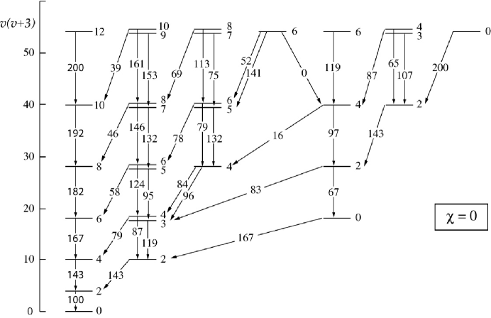
Figure 6: The low-energy spectrum of the Hamiltonian (36) in the SO(5) limit in which seniority $v$ is a good quantum number. Some pairs of degenerate energy levels are separated slightly for clarity. The $B$(E2) transition rates shown are in units such that $B({\rm E}2;12_{1}\to 00_{1})=100$. A more complete set of transition rates is given (precisely) in table 1. Quadrupole moments vanish for states of good seniority.

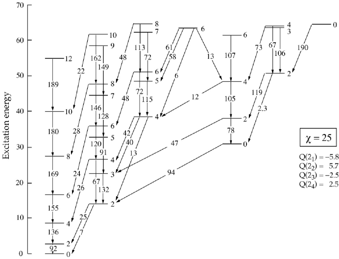
Figure 7: The low-energy spectrum and $B$(E2) transition rates for the Hamiltonian (36) with $\chi=25$. The units are as defined in the caption to fig. 6. For $\chi$ non-zero, seniority is no longer a good quantum number and quadrupole moments are no longer zero.

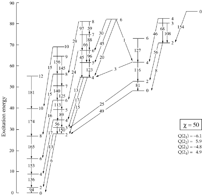
Figure 8: The low-energy spectrum and $B$(E2) transition rates for the Hamiltonian (36) with $\chi=50$. The units are as defined in the caption to fig. 6. For $\chi$ non-zero, seniority is no longer a good quantum number and quadrupole moments are no longer zero.

It is instructive to compare the results of fig. 8 with the sequence of rotational bands expected in the standard axially symmetric rotor model shown in fig. 9.

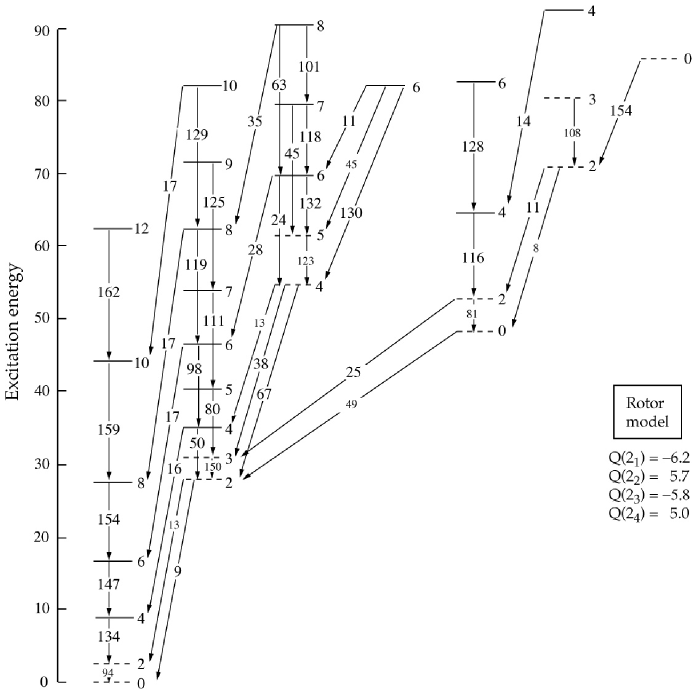
Figure 9: The low-energy spectrum and $B$(E2) transition rates given by the axially symmetric rotor model with band-head energies and moments of inertia adjusted so that the dashed energy levels are fitted to those of fig. 8. The intrinsic quadrupole moments of the model were also adjusted to fit the E2 transition rates shown in smaller type.

The comparison shows that the rotational dynamics are adiabatic relative to the gamma-vibrations for the lowest energy states but that significant departures become evident at higher energies. Increasing the value of $\chi$ would surely reduce the rotational-vibrational coupling and give results closer to those of the adiabatic rotor model. However, by the same token, the gamma-vibrational bands would rise to higher energies. It is of interest to see if some of the effects of rotation-vibration coupling, e.g. the non-rotational behaviour of some of the E2 transitions in the two-phonon $K=4$ gamma band, are realized in rotational nuclei having low-energy gamma bands. It would also be interesting to see if the results of fig. 8 can be reproduced more accurately in the adiabatic rotor model by taking the rotation-vibration coupling into account in perturbation theory.

VIII Summary

The Wilets-Jean model is an algebraic model with an ${\rm[R^{5}]SO(5)}\supset{\rm SO(5)}\supset{\rm SO(3)}$ dynamical subgroup chain. However, as observed above, the states that reduce this dynamical chain are strictly zero-width beta-rigid states. Complete rigidity is unphysical. Nevertheless, it is possible for the WJ model to work well even when the beta fluctuations of physical states are relatively large. This is because, it is hard to measure the beta-width of physical states; indeed it is invariably unclear as to the nature of excited $K=0$ excitations. Many intrinsic excitations of a nucleus can give rise to excited $K=0$ bands and even the collective model has two-phonon $K=0$ gamma bands.

To avoid the problems associated with the beta-rigidity of the WJ model, we considered in this paper a more physical collective model which, in its gamma-soft limit, has an ${\rm SU(1,1)\times SO(5)}\supset{\rm SO(5)}\supset{\rm SO(3)}$ dynamical subgroup chain. For large values of the parameter $\beta_{0}\sqrt{\omega}$, the low-energy states of this model acquire properties that are essentially indistinguishable from those of the less physical WJ model. In the WJ limit of this model, the beta vibrational frequency is infinite for a finite value of $\beta_{0}$ and, hence, beta vibrational excitations are not observable. However, neither an infinite beta-vibrational frequency nor a zero beta-width for collective wave function is necessary to obtain the results of the WJ model. All that is needed is an adiabatic decoupling of the rotational and beta-vibrational degrees of freedom. The signature of such decoupling is that the beta wave functions in the ${\rm SU(1,1)\times SO(5)}$ model become essentially independent of the excitation energy for the range of energies of interest. That such is the case when the rotational energies are small compared to the one-phonon beta-vibrational energy is illustrated in fig. 5.

Relaxing the rigidity of the WJ model and replacing its ${\rm[R^{5}]SO(5)}$ dynamical group with ${\rm SU(1,1)\times SO(5)}$, results in a more physical collective model. More importantly, it makes it possible to construct a basis in which arbitrary collective model Hamiltonians can be expanded in a rapidly convergent manner. For example, the solutions of the Hamiltonian (37) given in figs. 6-8 were obtained by diagonalization of $12\times 12$ matrices. For values of $\chi>50$, the dimensions would have to be increased to ensure accurate results. But clearly, much larger dimensions can be accommodated with available computers.

Appendix A The five-dimensional Kratzer model

The five-dimensional Kratzer model, proposed by Fortunato and Vitturi FV , has a similar algebraic solution to that of the Elliott-Evans-Park model EEP86 . A straightforward extension of the methods used for the hydrogen atom to the Hamiltonian

$$\hat{H}=-{\hbar^{2}\over 2B}\nabla^{2}-{k\over\beta}\,,$$ (65)

of a five-dimensional Coulomb problem gives the energy levels

$$E_{n\tau}=-{k^{2}B\over 2\hbar^{2}\nu_{n\tau}^{2}}\,,\quad\nu_{n\tau}=n+\lambda_{\tau}/2\,,$$ (66)

and wave functions

$$\Psi_{n\tau}(\beta)=\sqrt{n!\over\Gamma(n+\lambda_{\tau})2\nu^{6}_{\tau}b^{5}}\ \Big{(}{\beta\over b\nu_{\tau}}\Big{)}^{(\lambda_{\tau}-4)/2}\exp\Big{(}-{\beta\over 2b\nu_{\tau}}\Big{)}\,L^{(\lambda_{\tau}-1)}_{n}\Big{(}{\beta\over b\nu_{\tau}}\Big{)}\,\mathcal{Y}_{\tau\sigma}(\omega),$$ (67)

where now $\lambda_{\tau}=2\tau+4$ and $b=\hbar^{2}/(2kB)$.

These results are obtained by use of the SU(1,1) Lie algebra spanned by the operators

$$\hat{Z}_{1}=-2\beta\nabla^{2},\quad\hat{Z}_{2}=2\beta,\quad\hat{Z}_{3}=-2i(q\cdot\nabla+\textstyle{5\over 2})\,.$$ (68)

Again it is seen that, the commutation relations of this Lie algebra are unchanged if $\hat{Z}_{1}$ is replaced by

$$\hat{Z}_{1}^{\prime}=2\beta\Big{(}-\nabla^{2}+{\beta_{0}^{4}\over\beta^{2}}\Big{)}\,.$$ (69)

It follows that the above results for the Kepler Hamiltonian, extend immediately to the five-dimensional Kratzer model with Hamiltonian

$$\hat{H}(\varepsilon)={\hbar^{2}\over 2B}\Big{(}-\nabla^{2}+{\beta_{0}^{4}\over\beta^{2}}\Big{)}-{k\over\beta}\,.$$ (70)

However, now the relationship $\lambda_{\tau}=2\tau+4$ is replaced by

$$\lambda_{\tau}=1+2\sqrt{(\tau+\textstyle{3\over 2})^{2}+\beta_{0}^{4}}\,.$$ (71)

This follows because the replacement $\hat{Z}_{1}\to\hat{Z}_{1}^{\prime}$ in the SU(1,1) Lie algebra modifies the value of the SU(1,1) Casimir invariant from the value $\lambda_{\tau}(\lambda_{\tau}-2)=4\tau(\tau+3)+8$ to the value

$$\lambda_{\tau}(\lambda_{\tau}-2)=4\tau(\tau+3)+8+4\beta_{0}^{4}\,.$$ (72)

References

- (1) A. Bohr, Mat. Fys. Medd. Dan. Vid. Selsk. 26, no. 14 (1952); A. Bohr and B.R. Mottelson, ibid. 27, no. 16 (1953).
- (2) A. Bohr and B.R. Mottelson, Nuclear Structure, Vol. I, (Benjamin, Mass., 1969); – Vol. II (Benjamin, Mass., 1975)
- (3) D.J. Rowe, Nuclear Collective Motion: Models and Theory (Methuen, London, 1970).
- (4) J.P. Elliott, J.A. Evans and P. Park, Phys. Lett. 169B, (1986) 309; J.P. Elliott, P. Park and J.A. Evans, Phys. Lett. 171B (1986) 145.
- (5) D.J. Rowe and C. Bahri, J. Phys. A: Math. Gen. 31, 4947 (1998).
- (6) B.H. Flowers, Proc. Roy. Soc. A 210, 497 (1952); A 212, 248 (1952); A 215, 398 (1952).
- (7) A.K. Kerman, Ann. of Phys. 12, 300 (1961).
- (8) I. Talmi, Simple Models of Complex Nuclei Harwood, Chur, 1991).
- (9) J.P. Elliott, Proc. Roy. Soc. A245, 128, 562 (1958).
- (10) J.C. Parikh, Group Symmetries in Nuclear Structure, Nuclear Physics Monographs, eds. E.W. Vogt and J.W. Negele (Plenum, New York, 1978).
- (11) D.J. Rowe, Dynamical Symmetries of Nuclear Collective Models, Prog. Part. Nucl. Phys. 37, 265 (1996).
- (12) J.M. Eisenberg and W. Greiner, Nuclear Models, 3rd. edition (North Holland, 1987).
- (13) P.O. Hess, M. Seiwert, J. Maruhn, and W. Greiner, Z. Physik A – Atoms and Nuclei, 296, 147 (1980).
- (14) A. Arima and F. Iachello, Ann. Phys. 99, 253 (1976); 111, 201 (1978); O. Scholten, A. Arima and F. Iachello, Ann. Phys. 115, 325 (1978).
- (15) D.J. Rowe, Microscopic Theory of the Nuclear Collective Model, Rep. Prog. Phys. 48, 1419 (1985).
- (16) G. Rosensteel and D.J. Rowe, Phys. Rev. Letts. 38 10 (1977); Ann. of Phys. 126, 343 (1980).
- (17) C. Bahri and D.J. Rowe, Nucl. Phys. A 662, 125 (2000).
- (18) M.J. Carvalho, D.J. Rowe, S. Karram, and C. Bahri, Nucl. Phys. A 703, 125 (2002).
- (19) L. Wilets and M. Jean, Phys. Rev. 102, 788 (1956).
- (20) E. Chacon, M. Moshinsky, and R.T. Sharp, J. Math. Phys. 17, 668 (1976); E. Chacon, M. Moshinsky, J. Math. Phys. 18, 870 (1977)
- (21) L. Fortunato and A. Vitturi, preprint and private communication.
- (22) P.M. Davidson, Proc. Roy. Soc. London 135, 459 (1932).
- (23) S. Flügge, Practical Quantum Mechanics (Springer-Verlag, Berlin, 1971).
- (24) J. Čížek and J. Paldus, Int. J. Quant. Chem., XII, 875 (1977).
- (25) B.G. Wybourne, Classical Groups for Physicists (Wiley, New York, 1974).
- (26) T.H. Cooke and J.L. Wood, Am. J. Phys. 70, 945 (2002).
- (27) D.J. Rowe, P. Turner, and J. Repka, in preparation.
- (28) N. Kemmer, D.L. Pursey, and S.A. Williams, J. Math. Phys. 9, 1224 (1968).