A Genetic Algorithm Analysis of $N^{*}$ Resonances in $p\left(\gamma,K^{+}\right)\Lambda$ Reactions

Abstract

The problem of extracting information on new and known $N^{*}$ resonances by fitting isobar models to photonuclear data is addressed. A new fitting strategy, incorporating a genetic algorithm, is outlined. As an example, the method is applied to a typical tree-level analysis of published $p\left(\gamma,K^{+}\right)\Lambda$ data. It is shown that, within the limitations of this tree-level analysis, a resonance in addition to the known set is required to obtain a reasonable fit. An additional $P_{11}$ resonance, with a mass of about 1.9 GeV, gives the best agreement with the published data, but additional $S_{11}$ or $D_{13}$ resonances cannot be ruled out. Our genetic algorithm method predicts that photon beam asymmetry and double polarization $p\left(\gamma,K^{+}\right)\Lambda$ measurements should provide the most sensitive information with respect to missing resonances.

,

,

1 Introduction

The spectroscopy of baryons continues to be a subject of great interest in intermediate energy nuclear physics, since it an essential component in underpinning our knowledge of the substructure of the nucleon. Central to this is the issue of which resonances exist. Constituent quark models such as those proposed by Capstick and Roberts [1] predict a large number of resonances which thus far have not been observed, whilst for models which limit quark degrees of freedom [2], the number of “missing” resonances is less.

The majority of resonance information has been gleaned from analyses of single pion production reactions [3], and the suggestion that the missing resonances may couple more strongly to other channels [1, 4] has led to a number of experiments being proposed and carried out at intermediate energy accelerator facilities. Of particular interest is the possibility of studying strangeness production, since this opens up the possibility of extracting extra $N{}^{*}$ information.

The use of effective field theories is necessary in the resonance region since QCD cannot be solved perturbatively at this energy scale. Constituent quark models are able to predict quantities such as coupling constants and electromagnetic form factors, but it is not straightforward for these models to predict real observables, as a fundamental understanding of the underlying dynamics is missing. By using an effective field theory to extract coupling constants from fits to data, one can obtain numbers to compare with quark model predictions.

A complete understanding of the physics underlying the photonucleon data in the resonance region will in principle only be possible in a framework that contains all participating processes which include coupling to resonances [5, 6, 7, 8, 9]. This means taking into account meson production reactions such as $\gamma N\rightarrow\pi N,\>\pi\pi N,\>\eta N,\>\omega N,\>K\Lambda,\>K\Sigma,...,$ as well as Compton scattering and meson-induced production reactions. This is clearly an enormous task.

In a model adopting effective degrees-of-freedom, the field associated with each resonance has a number of free parameters which are usually determined by fitting model calculations to data. In a full-blown coupled-channels approach, the number of free parameters could easily end up being over 100. For such a procedure to be possible, a sizeable data set for each of the contributing channels is required. One difficulty, which is often overlooked, is the process of how to obtain a set of parameters which leads to the best description of the data. Related to this is the issue of how to assign error bars and confidence levels to the values of the extracted resonance parameters.

An analysis of a single channel, whilst not complete, offers the possibility of simplifying the problem by reducing the number of free parameters to a manageable size, and in being able to identify the most important features. Recent attempts to analyse the $p(\gamma,K^{+})\Lambda$ channel in such a framework have highlighted the tantalising prospect that previously undiscovered resonances may reveal themselves in the mechanisms involving strangeness production. Mart and Bennhold [10] used their tree-level hadrodynamical model to show that the total cross-section measured at SAPHIR [11] could be reproduced by introducing a $D_{13}(1895)$ resonance. This resonance does not appear in the Particle Data Group baryon summary table as it had not been conclusively observed, but was included in [10] because of the predicted coupling [1] to strange channels. In addition to this, a recent re-analysis of pion photoproduction data [12] appeared to find evidence for it. On the other hand, an analysis by Saghai [13] argued that by tuning the background processes involved, the need for the extra resonance was removed. Both approaches were based on the analysis of the SAPHIR data set, which at that point amounted to around 100 data points.

In a previous article [14], we highlighted the problem of extracting reliable resonance information from the limited set of $p(\gamma,K^{+})\Lambda$ data points by performing many independent fitting calculations. Using a fitting strategy based on a genetic algorithm we illustrated that a large number of different solutions resulted in similar $\chi^{2}$ values. We were able to group these solutions into two main sets: one with $D_{13}$ coupling constants close to zero (indicating its non-existence), and one with significantly non-zero $D_{13}$ coupling constants (indicating its existence). We further showed that the measurement of polarization observables, such as photon beam asymmetry, could have a pivotal role in removing ambiguities.

We have now performed a systematic study into the feasibility of determining the combination of resonances which contribute to the $p(\gamma,K^{+})\Lambda$ reaction. To this end, we have used a typical tree-level description of the reaction process in combination with a minimization procedure which is specifically designed to quantify the relative success of different combinations of resonances. This procedure employs a genetic algorithm which is able to search efficiently a large parameter space, coupled with a conventional minimization routine to ensure convergence. We have benefitted from adding new photon beam asymmetry measurements from SPring-8 [15], as well as fitting electroproduction data measured at Jefferson Lab [16].

The structure of this paper is as follows. We outline the features of a typical tree-level $p(\gamma,K^{+})\Lambda$ reaction model in section 2. Section 3 describes a framework which enables the extraction of resonance information from existing photonucleon data, and discusses how to evaluate the reliability of the information. As an example, the methodology is applied to a tree-level analysis of $p(\gamma,K^{+})\Lambda$ in section 4. We discuss the results of our work and highlight the important next steps in studying this problem. We present conclusions in section 5.

2 Model Formalism

We adopt a hadrodynamical framework for modelling kaon photoproduction on the nucleon. The model we use has been described in previous work [17], so we present only a brief summary here. The $p(\gamma,K^{+})\Lambda$ reaction process is described by hadronic degrees of freedom using an effective Lagrangian. The contributioning diagrams are depicted in figure 1. Every intermediate particle in the reaction is treated as an effective field with associated mass, photocoupling amplitudes and strong decay widths. Tree level Feynman diagrams contain the vector $K^{*}(892)$ and the axial-vector $K_{1}(1270)$ t-channel mesons, as well as the usual Born terms. Two hyperon resonances, the $S_{01}(1800)$ and $P_{01}(1810)$ are present in the u-channel. These ingredients constitute the so-called “background”.

Figure 1: Diagrams contributing to the $p(\gamma,K^{+})\Lambda$ process at the tree level. The upper row corresponds to the Born terms in which a proton is exchanged in the s-channel, a $\Lambda$ or $\Sigma^{+}$ in the u-channel, and a $K^{+}$ in the t-channel. The lower row shows the corresponding diagrams with the exchange of an excited particle or resonance.

In Ref. [18] we stressed the difficulties associated with parameterizing the background diagrams in $p(\gamma,K^{+})\Lambda$ calculations and presented results for three plausible background schemes. Subsequent work [19] showed that the $p(e,e^{\prime}K^{+})\Lambda$ process is highly selective with respect to viable choices for dealing with the background diagrams. The model used here is the only one which we found to reproduce simultaneously the $p(\gamma,K^{+})\Lambda$ and $p(e,e^{\prime}K^{+})\Lambda$ data.

The finite extension of the meson-baryon vertices is implemented by the use of hadronic form factors [20, 21, 22]. We also note in passing that the validity of this approach is only likely to be reasonable for photon energies below about 2 GeV, but its precise range of applicability remains to be established.

For the purposes of the present work, we have defined several versions of our hadrodynamical model which correspond to different choices of s-channel resonances. For brevity, we subsequently refer to these as different model variants, but the fact that they are based on the same hadrodynamical framework should be kept in mind. Each variant includes a “core” set of resonances, consisting of $S_{11}(1650)$, $P_{11}(1710)$ and $P_{13}(1720)$ which are well known to contribute to the $p(\gamma,K^{+})\Lambda$ reaction [10, 13, 23]. The variant containing only these resonances is referred to as the “Core” variant.

The other model variants each contain one other resonance of mass 1895 MeV. A $D_{13}$ resonance was chosen to be compatible with our earlier work and because it had been proposed in [10]. This in turn was motivated by the quark model of Capstick and Roberts [1] which showed that the $D_{13}$ had the largest coupling strength to the lowest spin states. However, rather than relying on the predictions of a constituent quark model calculation, we have tried different variants which contain a resonance of the same mass but alternative quantum numbers. If another resonance does contribute, the exact value of its mass is not likely to be important. Each of these variants is thus referred to by the character of the additional resonance: $S_{11}$, $P_{11}$, $P_{13}$ and $D_{13}$ . Our previous analysis only used Core plus $D_{13}$ resonances [14].

We therefore have set up our programme of calculations to address the questions of whether an additional resonance is required in the description of the reaction (Core versus non-Core variants), and what character an additional resonance might have ($S_{11}$, $P_{11}$, $P_{13}$ and $D_{13}$ variants).

3 Analysis Procedure

For each model variant, we performed a set of calculations to extract $N^{*}$ information from the reaction data. Each set consisted of 100 separate minimization calculations. The data sets employed in the fitting procedure included total cross-sections, differential photo-production cross-sections and recoil polarizations from the SAPHIR data set [11], and photon beam-polarization asymmetries from SPring-8 [15]. In addition, we also used separated longitudinal and transverse electroproduction data from Jefferson Lab [16], as well as total electroproduction cross sections from a variety of older sources [24, 25, 26].

The coupling constants associated with the hadronic vertices in all the amplitudes included in the model are free parameters in the fitting procedure. A description of their exact definition is given in [27], but we briefly list them here for completeness: coupling constants related to Born terms, $g_{K^{+}\Lambda p}$ and $g_{K^{+}\Sigma p}$; vector and axial vector mesons in the $t-$channel, $G_{K^{*}}^{v}$, $G_{K^{*}}^{t}$, $G_{K_{1}}^{v}$ and $G_{K_{1}}^{t}$; spin-$\frac{1}{2}$ $Y^{*}$ resonances in the $u-$channel, $G_{Y^{*}Kp}$; spin-$\frac{1}{2}$ $N^{*}$ resonances in the $s-$channel, $G_{N^{*}K\Lambda}$; spin-$\frac{3}{2}$ $N^{*}$ resonances in the $s-$channel, $G^{1}_{N^{*}K\Lambda}$, $G^{2}_{N^{*}K\Lambda}$ and three off-shell parameters. Note that these constants are products of both a hadronic part and an electromagnetic part. Two hadronic cut-off parameters (one for all the Born terms, $\Lambda_{born}$, and and for all resonances in the $s-$, $t-$ and $u-$ channels, $\Lambda_{res}$) are also free parameters.

To compare the relative success of each model variant in describing the data, we require two separate but related procedures: a search for the best set of free parameters for each model variant, and a comparison amongst the different model variants. The first procedure is achieved by varying the free parameters and searching for a minimum $\chi^{2}$ statistic by fitting calculations to the data. This is a fairly standard procedure, but we remind the reader in passing the assumptions which are implicitly required: the data points being fitted must be independent (the value of one does not affect the others), and error bars on the points represent the standard deviations of a Gaussian probability density. Both these requirements are likely to be approximately correct, and thus minimising $\chi^{2}$ is equivalent to maximising a likelihood function. The likelihood represents the probability that the data would be measured, given a particular set of free parameters.

Furthermore, there is the assumption that no particular values of the free parameters are to be favoured prior to the fitting procedure. By imposing limits on the free parameters (as we do through physics constraints) this is not strictly true, but will be approximately true if the limits are sufficiently large. The whole procedure is then equivalent to maximising the probability that a particular set of free parameters is correct, given the experimental data, by varying the free parameters.

Comparing different model variants needs to be done carefully, since each one may have a different number of free parameters. The approach we take implicitly employs “Occam’s razor” by penalising model variants with more free parameters.

3.1 Fitting

Each model variant has at least 20 parameters which need to be extracted by fitting the calculations to the data. Traditional optimizing routines require a first guess at parameter values. Whilst some prior experience can be used to estimate the starting values, in a parameter space of this size it is very difficult to judge whether an optimum found by an optimizer is local or global. In previous work [17] a simulated annealing strategy was adopted, however we subsequently found [14] that using a genetic algorithm (GA) in combination with a traditional optimizer, MINUIT [28], offered many advantages. The GA is able to search a large region of parameter space and very quickly arrives at reasonable solutions, whereas a minimizer such as MINUIT, which uses a Davidon-Fletcher-Powell algorithm, is able to take the solutions from the GA as starting points and find optima, provided the starting points are not too far from the optimum. This strategy thus plays to the strengths of both algorithms.

Genetic algorithms are a class of search strategies known as evolutionary computing. A number of excellent texts on GAs exist (e.g. [29, 30]), so we will only briefly sketch the strategy we have employed. The idea is to generate a number of trial solutions randomly. In this implementation, each solution is an encoding of trial values of the free parameters as a string of real numbers $\left\{\lambda_{i}\right\}$, where $\lambda_{i}$ represents the value of free parameter $i$.

The collection of solutions is referred to as a “population”. Each solution in the population is used to evaluate a function which determines its “fitness”. In our case the fitness function is

$$f\left\{\lambda_{i}\right\}=\frac{1}{1+\chi^{2}\left\{\lambda_{i}\right\}},$$

where $\chi^{2}\left\{\lambda_{i}\right\}$ is the result of running the calculation of all the experimental observables and comparing with the available data.

The population is then “evolved” in a manner analogous to biological evolution. One or two solutions are selected from the current population, where solutions with greater fitness function values are selected preferentially, but not exclusively. When one solution is selected, it is subjected to a “mutation”, where one or more of the free parameters are altered at random.

When two solutions are selected, a new individual is created by “crossover” of the encoded parameters in each solution. In this implementation, crossover is performed by a number of different functions, chosen at random, which fall broadly into two categories. The first is to swap one or more parameters from solution $\left\{\lambda_{i}\right\}$ to solution $\left\{\mu_{i}\right\}$, $\lambda_{i}\leftrightarrow\mu_{i}$ two obtain two “child” solutions. The second takes parameters from each solution and forms one child by assigning it new parameters $\left\{\nu_{i}\right\}$ calculated by a weighted averaged: $\nu_{i}=\frac{w_{1}\lambda_{i}+w_{2}\mu_{i}}{w_{1}+w_{2}}$.

A new fitness is then evaluated, and if it is better than the worst current fitness in the population, the new solution replaces the previous worst. This is often referred to as a steady state GA. The population therefore gradually migrates to one or more better points in parameter space, and if the routine is run for long enough, it will converge on one optimum. Whilst this optimum is not guaranteed to be global, GA research [30] has shown that “reasonable” solutions can be found very efficiently, even when no prior information has been used to constrain the free parameters. For instance, in our calculations, the best-of-generation solutions at the start of a run have $\chi^{2}$ values of order $10^{6}$ but this will be reduced to of order 10 after only 5000 evaluations of the objective function. If gradient methods were employed using such a random choice of initial starting values, it is highly likely they would be trapped in local minima. Note also that compared to the simulated annealing strategy used in previous work [17, 18, 19, 31] we have reduced the number of function evaluations by a factor of 10. Whereas no one strategy can be optimum for all problems, the GA is likely to be highly efficient for problems such as the present one with many parameters and complicated $\chi^{2}$ surfaces. The best-of-generation solutions at the end of each GA run can be used as starting points for a MINUIT minimization.

The complete strategy for analysis of each model was as follows:

1. 100 GA calculations were initiated. Each GA calculation used a population of 200 and was run for 5000 evaluations of the objective function. The limits for each parameter were deliberately chosen to define a large region of parameter space.

2. The best solution from each GA calculation was used as a starting point for a MINUIT minimization which was run for a further 5000 function evaluations. At this point very few, if any, of the MINUIT calculations had achieved convergence and the residual values of $\chi^{2}$ were too high; a more limited search space was required.

3. The parameters associated with each of the 100 MINUIT solutions were then examined. The set of solutions whose $\chi^{2}$ values were within 1.0 of the current best $\chi^{2}$ were selected. A new, tighter set of limits for each parameter was defined from the range of parameter values exhibited by the chosen subset of solutions. This typically reduced parameter ranges by factors of 5-10.

4. 100 new GA calculations were initiated, the only difference from before being the smaller region of parameter space in which the search was performed.

5. As before, the best solution from each GA calculation was used to initiate MINUIT calculations. A few calculations had converged at this point. It was clear, however, that the calculations had not converged to the same optimum, so to investigate this, we proceeded to try to obtain convergence for all the calculations.

6. The MINUIT solutions were then re-inserted back into the GA populations. Since the inserted solution was likely to be the “fittest” solution in the population, this would cause the GA to concentrate more on a particular region of parameter space. Furthermore, the populations from each of the 100 GA calculations were mixed. This is a variation on what is known as an island population mixing scheme, and can be shown to be beneficial in cases where separate GAs are converging on different optima.

7. A third run of the 100 GA calculations was now performed.

8. A final MINUIT calculation for each of the 100 GA best solutions was done. At this point, all the calculations had converged.

The result for each model variant was 100 solutions, each of which represented a converged minimization by MINUIT. As we noted in [14], we observed that each solution was unique, even although they had roughly similar $\chi^{2}$ values. In other words, there were at least 100 local minima in the $\chi^{2}$ surface.

The fact that each calculation appears to find a different local minimum shows that the optimization problem may be ill-posed. The reason for this could be either that the reaction model lacks an ingredient which is necessary to obtain reproducible minimization results, or that the experimental data contain systematic uncertainties which render them inconsistent with each other, or that both the model and the data are problematic. From this observation, we caution that it is not possible to extract the magnitudes of coupling constants to high precision by fitting hadrodynamical models such as ours (and by extension other similar models) to a relatively small number of photoproduction data points.

What is observed however, is that the “best” of the calculations (i.e. those with the lowest $\chi^{2}$ values) tend to cluster around particular regions in parameter space. Our previous work [14] showed that this still resulted in considerable ambiguities in the calculations of un-measured observables, and pointed to quantities such as photon asymmetry as being very useful in reducing the uncertainties in parameter values. The additional data used in the present work are the beam polarization data from the SPring-8/LEPS facility [15] and electroproduction data [16, 24, 25, 26], and it appears they have affected a marked reduction in the regions of parameter space which give a good fit to the data (see section 4). This is a valuable observation. It shows that our original work, in agreement with others (e.g. [10]), was able to predict the measurements which would most significantly improve the comparison between data and theory.

3.2 Model Variant Comparison

Whilst the best fit for each model was obtained by minimising $\chi^{2}$, this does not take into account the different number of free parameters in each model, or how small a region of parameter space corresponds to a reasonable fit. A full description of the framework we have employed is given in the appendix, but we sketch the salient points here.

Comparing two model variants ($A$ and $B$, say), we can evaluate the ratio of the likelihood functions:

$$\frac{P\left(D|A\right)}{P\left(D|B\right)}\,,$$ (1)

where $P\left(D|A\right)$ ($P\left(D|B\right)$ ) is the probability that the data $D$ would be obtained, assuming that variant $A$ ($B$) were true. Under some reasonable assumptions (as mentioned previously), minimising $\chi^{2}$ is equivalent to maximising the likelihood, but what is actually obtained could be written as $P\left(D|\lambda_{i}^{MP},A\right)$ (where $MP$ stands for “most probable”). This expression indicates that the maximum likelihood depends on the parameters of the model, $\lambda_{i}$, whereas Eq.1 requires there to be no dependence on the free parameters of either variant.

Using further approximations, we obtain for variant $A$ the expression (with a similar one for variant $B$):

$$P\left(D|A\right)\propto P\left(D|\lambda^{MP},A\right)\frac{\prod_{i}^{N}\delta\lambda_{i}^{MP}}{\prod_{i}^{N}\left(\lambda_{i}^{max}-\lambda_{i}^{min}\right)}\,,$$ (2)

where there are $N$ free parameters, $\lambda_{i}^{max}$ and $\lambda_{i}^{min}$ represent the maximum and minimum limits of search space for parameter $\lambda_{i}$, and $\delta\lambda_{i}^{MP}$ is the uncertainty in the most probable value of parameter $\lambda_{i}$. The second factor in Eq.2 is often referred to as the “Occam factor”, since it penalizes model variants with more free parameters. It is most easily interpreted as a product of $N$ factors, each one a ratio of fitted error bar size to search space size for parameter $\lambda_{i}$. Model variants whose parameter error bars are relatively large are thus more favoured by the data since it means that there is a larger region of parameter space which gives a good fit of the model to the data. The ratio in equation 1 becomes not just a ratio of maximum likelihoods, but is multiplied by the ratio of Occam factors.

Coupling constants associated with the Born amplitudes and the cutoff parameters were free parameters in the fitting procedure, but tended to migrate to limits imposed by physical considerations such as SU(3) symmetry. However, for all model variants these parameters were roughly similar, and so were “uninteresting” from a physical point of view. We therefore reduced the effective number of free parameters after the fitting procedure by considering only those parameters which related are to coupling constants of resonances in the $s$-channel.

4 Results and discussion

4.1 Fits to the available data

The results from the fitting calculations are summarized in table 1. The factors quoted in the table are described as follows:

1. $\chi^{2}$: The value quoted is the lowest $\chi^{2}$ per data point found for each model variant.

2. Number of free parameters: This is the number of $s$-channel resonance coupling constants which were varied in the fitting procedure, as explained in section 3.

3. Number of “best” calculations: For each model variant, a histogram of the number of calculations versus $\chi^{2}$ was produced. Fig. 2 shows three such histograms representing the results from the $P_{11}$, $P_{13}$ and $D_{13}$ model variants. Remembering that each calculation is a converged MINUIT result, it can be seen that there is a range of $\chi^{2}$ values for each variant. Examination of figure 2 reveals significant differences in the results according to model variant. For instance, $P_{11}$ shows a large number of calculations at one value of $\chi^{2}$ (at the level of histogram binning), whereas $P_{13}$ shows a much wider range in $\chi^{2}$, but there is one calculation which has attained a much better $\chi^{2}$ than all the others, and $D_{13}$ is somewhere in between the two. One can also see that $D_{13}$ contains calculations with the lowest $\chi^{2}$, but there are only a handful of them, whilst $P_{11}$ has a large fraction of its calculations in the lowest $\chi^{2}$ “peak”. The number of best calculations represents the number in the lowest $\chi^{2}$ “peak” for each model variant.

4. Occam factor: The Occam factors are also included to show how the various model variants are penalized for having either a larger number of free parameters, or which obtain good fits only in a smaller region of parameter space. They are normalized to the value obtained for the “Core” variant.

5. Ratio of Posterior Probabilities: The figures quoted are the result of applying the formulae derived in section 3 and the appendix. As with the Occam factor, they are also normalized to the value obtained for the “Core” variant.

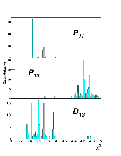
Figure 2: Histograms of the number of calculations resulting in $\chi^{2}$ values

Model Variant	Core	$S_{11}$	$P_{11}$	$P_{13}$	$D_{13}$
$\chi^{2}$	5.14	4.47	3.47	3.75	3.35
Number of free parameters	4	5	5	6	6
Number of “good” calculations	15	1	64	1	8
Occam factor	1.000	3.278	5.556	0.018	1.167
Ratio of Posterior Probabilities	1.000	4.500	12.571	0.035	2.786

Table 1: Results from the fitting calculations. The various factors are explained in the text.

The “raw” $\chi^{2}$ results show that the $D_{13}$ model variant gives the best fit to data (in agreement with other predictions [10]), but that the $P_{11}$ and $P_{13}$ variants also give comparable fits. However, once the Occam factor is taken into account, the ratio of posterior probabilities show that the $P_{11}$ variant is favoured by a factor of 4.5 over $D_{13}$ and a factor of 359 over $P_{13}$. It is interesting to note that this mirrors the “intuitive” feeling we obtained when examining the distributions of $\chi^{2}$ results shown in figure 2, i.e. the model variant with the greater number of low $\chi^{2}$ calculations ($P_{11}$) is favoured over the one with very few ($P_{13}$). It is also interesting to note that $S_{11}$ is slightly favoured over $D_{13}$, even although the raw fit to data is not as good; this presumably reflects the fact that $D_{13}$ contains more parameters than $S_{11}$.

The main points we would like to conclude from this are:

1. The available data show evidence that, within our model framework, an additional resonance is required.

2. The quantum numbers of the additional resonance are not possible to ascertain (given the amount of experimental data), but the present data set give greatest support to the hypothesis that it is a $P_{11}$.

4.2 Comparison with the data used in the fitting procedure

In order to show how well each model variant can fit the data, we present a selection of plots which show the comparison. For each variant, the parameters found by the fitting calculation which produced the best $\chi^{2}$ value have been used. Our previous work [14] showed calculations using many different fitted parameter sets to make the point that a great deal of ambiguity remained after fits to data. However, now that we have included new data points in the fitting process, namely the photon beam asymmetry and electroproduction data, the ambiguity in parameters within the same model has been drastically reduced. We therefore restrict ourselves to plotting one calculation for each model variant, since the differences within a model variant are much smaller than the differences amongst the different variants.

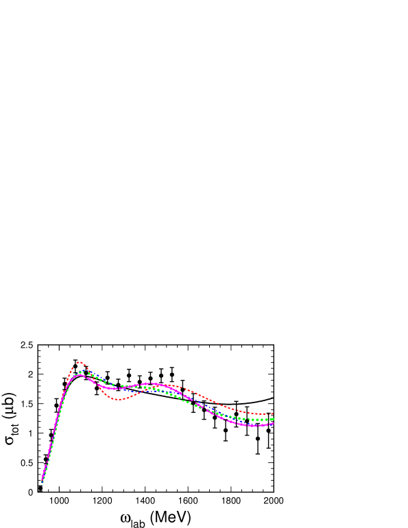
Figure 3: Total cross-section for the $p(\gamma,K^{+})\Lambda$ reaction. The data points are from [11]. The model variant calculations are: core set (solid line), $S_{11}$ (dashed line), $P_{11}$ (small circles), $P_{13}$ (dot-dashed line) and $D_{13}$ (solid plus circles).

Figure 3 shows the comparison of all the model variants to the total $p(\gamma,K^{+})\Lambda$ cross-section data, whilst figures 4 and 5 show typical differential cross-section and recoil polarization fits respectively. At this point we note that the four model variants which include an additional resonance are able to reproduce a “resonant bump” in the total cross-section, whilst the core variant cannot.

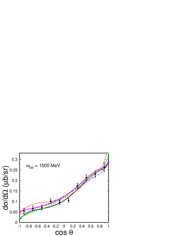
Figure 4: Fit of each model variant to differential cross-section data. The lines have the same meaning as in figure 3.

The recoil polarizaton in figure 5 again shows that an additional resonance is required in order to reproduce the data especially at backward angles. Whilst a “bump” in the total cross-section was reproduced by Saghai [13] by altering an ingredient of the background processes, it is unlikely that the tuning of the background could result in a substantial non-zero recoil polarization as seen in the data. This observation may be a further indication that an additional resonance is required in this energy range.

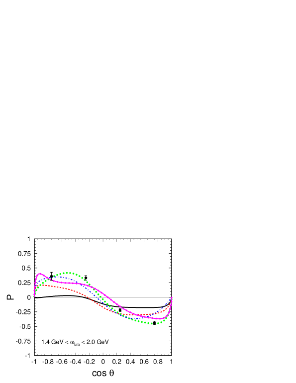
Figure 5: Fit of each model variant to the recoil polarisation data. The lines have the same meaning as in figure 3.

Figure 6 shows the calculations compared to the recent SPring-8 photon asymmetry [15]. It is clear that these data have greatly influenced the overall fit, since they tie down all the calculations at forward angles. Indeed, we predicted that this would be the case [14]. However, especially at the lower energy setting (1.55 GeV), it is still the case that there is a large difference in the model calculations over most of the angular range. Measurements over an extended range of angle would therefore be very useful to constrain further the fitting procedure. At 1.55 GeV, even an asymmetry averaged over the entire angular range would discriminate between the $P_{11}$ and $D_{13}$ calculations, since the predictions are negative and positive respectively.

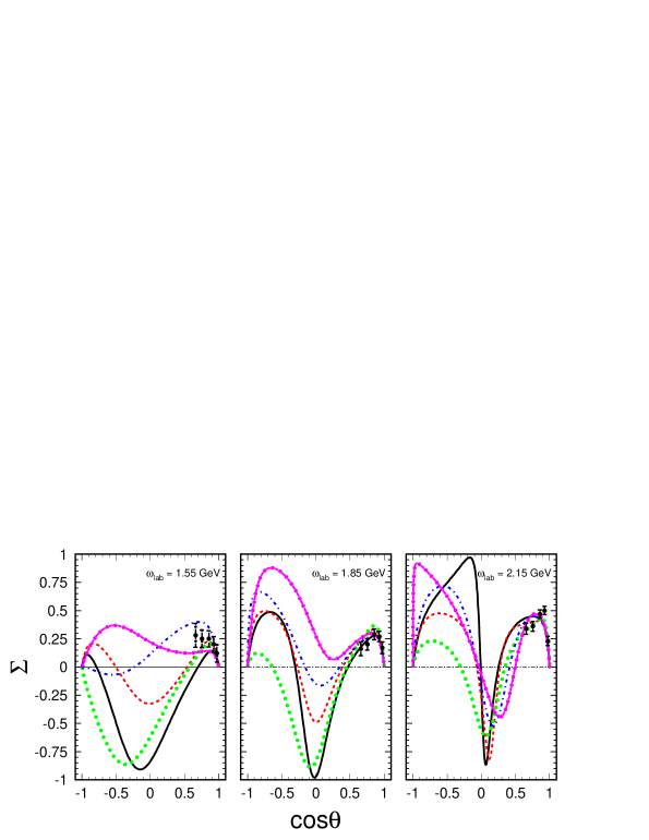
Figure 6: Fit of each model variant to photon beam asymmetry data. The data are from [15], and the lines have the same meaning as in figure 3.

Comparisons with electroproduction data are presented in figure 7. Longitudinal, transverse and combined differential cross-sections are shown. It is clear that agreement with the transverse cross section is the least good of all the comparisons with data, and is probably responsible for the residual high values of $\chi^{2}$ found in the fitting process. However, we note that there is virtually no difference amongst the model variants in the combined cross-sections, and only a small scale and form difference in the separated cross-sections. In other words, these electroproduction observables are relatively insensitive to details of the resonances in the reaction, and mirror our previous work [19] where we concluded that they are highly influenced by “background” processes.

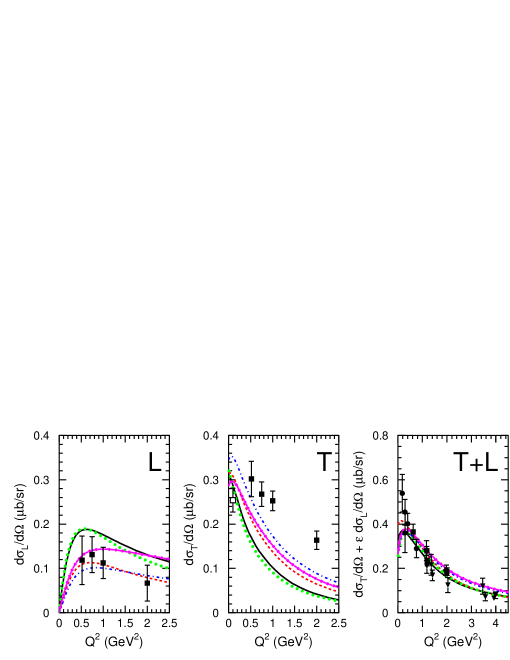
Figure 7: Fits of model variants to electroproduction data. The separated longitudinal (L) and transverse (T) differential cross section filled square data are from [16] at $W=1.84$GeV and $\theta_{qK}^{\star}=0^{\circ}$, and the $Q^{2}=0$ (photoproduction point) from [11] is shown as a comparison. The combined (T+L) differential cross-section data are from [24, 25, 26] at $W=2.15$GeV and $\theta_{qK}^{\star}=8^{\circ}$. The lines have the same meaning as in figure 3.

For completeness, and to summarize the results of our analysis, we show in table 2 the values of the resonance coupling constants which correspond to the best fit calculation for each model variant. In addition, we show graphically the range and correlation of the coupling constant values in figure 8, for those coupling constants which are common to all models. Error bars (where shown) indicate the spread (standard deviation) of the values for the “best” calculations, defined in table 1, otherwise the spread is less than the size of the symbol. This plot indicates that the values extracted from the process are indeed highly correlated with the choice of additional resonance, as there are no discernable similarities in values and there is also a sizeable spread.

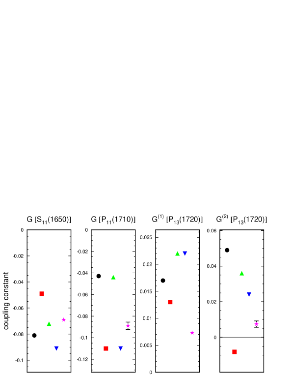
Figure 8: Depiction of the values of the main coupling constant found for each model variant. The meaning of the symbols are: circle - core set, square - $S_{11}$, upright triangle - $P_{11}$, downwards triangle - $P_{13}$ and star - $D_{13}$.

	Model Variant
Coupling Constant	Core	$S_{11}$	$P_{11}$	$P_{13}$	$D_{13}$
$G[S_{11}(1650)]$	$-8.1\times 10^{-2}\pm 3.6\times 10^{-5}$	$-4.9\times 10^{-2}$	$-7.2\times 10^{-2}\pm 2.1\times 10^{-4}$	$-9.1\times 10^{-2}$	$-6.9\times 10^{-2}\pm 2.2\times 10^{-4}$
$G[P_{11}(1710)]$	$-4.3\times 10^{-2}\pm 9.4\times 10^{-5}$	$-1.1\times 10^{-1}$	$-4.4\times 10^{-2}\pm 1.4\times 10^{-3}$	$-1.1\times 10^{-1}$	$-8.9\times 10^{-2}\pm 3.5\times 10^{-3}$
$G^{(1)}[P_{13}(1720)]$	$1.7\times 10^{-2}\pm 1.2\times 10^{-5}$	$1.3\times 10^{-2}$	$2.2\times 10^{-2}\pm 1.6\times 10^{-4}$	$2.2\times 10^{-2}$	$7.3\times 10^{-3}\pm 2.8\times 10^{-4}$
$G^{(2)}[P_{13}(1720)]$	$4.9\times 10^{-2}\pm 6.0\times 10^{-5}$	$-8.2\times 10^{-3}$	$3.6\times 10^{-2}\pm 6.9\times 10^{-4}$	$2.4\times 10^{-2}$	$7.4\times 10^{-3}\pm 1.8\times 10^{-3}$
$G[S_{11}(1895)]$	-	$8.7\times 10^{-2}$	-	-	-
$G[P_{11}(1895)]$	-	-	$-3.8\times 10^{-1}\pm 5.5\times 10^{-4}$	-	-
$G^{(1)}[P_{13}(1895)]$	-	-	-	$2.1\times 10^{-2}$	-
$G^{(2)}[P_{13}(1895)]$	-	-	-	$2.1\times 10^{-2}$	-
$G^{(1)}[D_{13}(1895)]$	-	-	-	-	$-2.2\times 10^{-1}\pm 5.7\times 10^{-4}$
$G^{(2)}[D_{13}(1895)]$	-	-	-	-	$-2.5\times 10^{-2}\pm 8.0\times 10^{-4}$

Table 2: The values of the coupling constants extracted from the fitting procedures.

4.3 Comparisons with other data

A recent experiment using the CLAS detector at Jefferson Lab [32] has measured the transferred polarization in the exclusive $p(\vec{e},e^{\prime}K^{+})\vec{\Lambda}$ reaction. Figure 9 shows the comparison of the model variants with this data set. We have not used this data in the fitting routine because the calculation of each point would require an averaging over the phase-space of each data bin, thereby significantly increasing the computational time. Instead we show the predictions for each model variant, based on the extracted free parameters described in 4.2. All the calculations show moderate agreement with the data, with the exception of the $P_{x}^{\prime}$ observable which was measured to be consistent with zero, where none of the model variants appear to be able to reproduce this behaviour. It was suggested in [32] that this may be due to the production of $s\bar{s}$ quark pairs with anti-aligned spins. This is beyond the scope of the present hadrodynamical model. However, in common with the separated longitudinal and transverse differential cross-sections, there is relatively little sensitivity to details of which resonances are included in the reaction calculations, which indicates that this reaction is not best one to search for missing resonances.

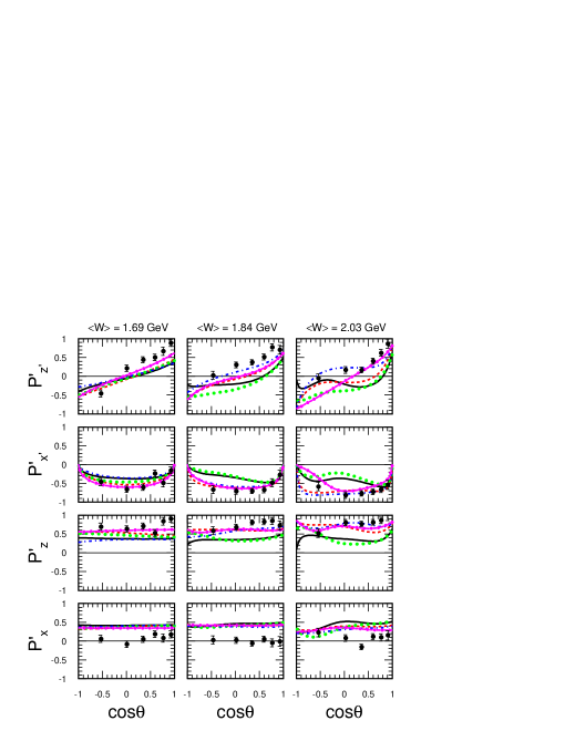
Figure 9: Comparison with the double polarization electroproduction data of ref. [32]. The line conventions are the same as Fig. 3.

4.4 Predictions for other observables

We have already seen that a more comprehensive measurement of the photon beam asymmetry would be highly sensitive to the choice of resonance in the reaction. With the prospect of double polarization photoproduction experiments [33], we present some predictions, based on the models described above and using the parameters found in the fitting procedures. The authors of [33] have proposed to measure beam-target, target-recoil and beam-recoil polarizations for both $p(\gamma,K^{+})\Lambda$ and $p(\gamma,K^{+})\Sigma$ reactions at a photon beam energy of 1.5 GeV.

Figures 10 and 11 show the results of the calculations using each of our models of beam-recoil and beam-target polarization for the $p(\gamma,K^{+})\Lambda$ reaction only. Beam-target, target-recoil and beam-recoil polarizations are not independent, although in practice the measurement of all three would be desirable to limit systematic effects. All the observables show a high degree of sensitivity to the choice of resonance. One could therefore imagine that the measurement of a few selected points would be highly valuable in determining the dynamics of the reaction.

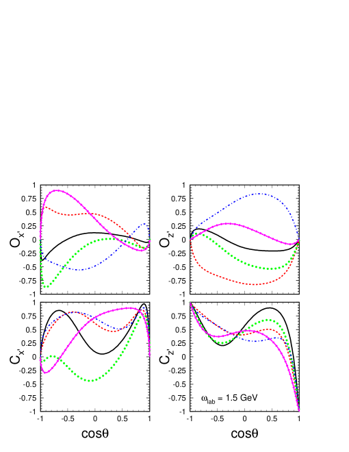
Figure 10: Beam-recoil polarization prediction for linearly (top panels) and circularly (bottom panels) polarized photons.

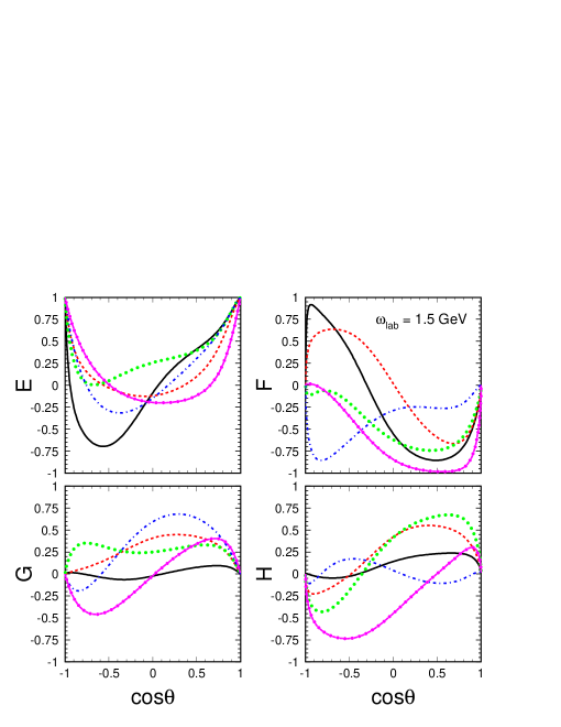
Figure 11: Beam-target polarization prediction for circularly (top panels) and linearly (bottom panels) polarized photons.

5 Conclusion

A framework for analysing $p(\gamma,K^{+})\Lambda$ reaction data sets has been presented. Using the foundation of a tree-level hadrodynamical model, we have shown that the extraction of coupling constants by fitting to data is not trivial. The strong suggestion from our work is that fitting procedures should be carried out several times in order to establish how reliable the extracted numbers are. Carrying out the fitting procedure using a hybrid of a genetic algorithm and a traditional minimizer has been shown to play to the strengths of both strategies, and carrying out many calculations in parallel allows a thorough investigation of the character of the search space. Any conclusions from such procedures must take into account the uncertainty resulting from calculations which converge on different optima in parameter space.

From the analysis shown here, we have reasonable evidence that an extra resonance is required to explain the $p(\gamma,K^{+})\Lambda$ reaction data within our model. The study shows that the data currently favour the presence of an additional $P_{11}$ resonance of mass 1895 MeV, but that $S_{11}$ and $D_{13}$ resonances are also weakly supported and cannot therefore be ruled out. We have not studied how combinations of additional resonances might improve the description. A firm conclusion awaits further data and a full-blown theoretical coupled-channel analysis to pin down the remaining uncertainty. There is a strong possibility that a GA may be of great value in the minimization required in a coupled-channel approach.

We have shown that whilst the different model variants do a reasonable job of describing the $p(e,e^{\prime}K^{+})\Lambda$ data, they are relatively insensitive to the details of the contributing resonances. The polarization observables in photoproduction reactions remain the best candidates for investigating the nature of any additional resonances.

We are aware that further comprehensive data sets have been published [34, 35]. We look forward to being able to use this to improve the quality of the information extracted in our approach. In addition, the inclusion of radiative kaon capture data [36] may provide further constraints on the values of resonance couplings. However, we note that in this reaction, which is crossed-symmetric to the $p(\gamma,K^{+})\Lambda$ studied above, coupled channel effects have been shown to be important [37, 38].

This work was supported by the UK’s Engineering and Physical Sciences Research Council, and the Fund for Scientific Research - Flanders.

Appendix: Model comparison

We compare the relative success of the different model variants by evaluating the ratios of the maximum posterior probabilities [39]. To compare variants $A$ and $B$ the ratio, after application of Bayes Theorem, becomes

$$\frac{P\left(A|D\right)}{P\left(B|D\right)}=\frac{P\left(D|A\right)P\left(A\right)}{P\left(D|B\right)P\left(B\right)}\,,$$

where $P\left(A|D\right)$ is the maximum posterior probability for variant $A$, $P\left(D|A\right)$ is the probability that the data would be obtained, assuming variant $A$ to be true, $P\left(A\right)$ is the a priori probability that variant $A$ is correct and similarly for variant $B$. With no prior prejudice as to which variant is correct, we obtain the ratio of likelihoods:

$$\frac{P\left(D|A\right)}{P\left(D|B\right)}\,.$$

The likelihood $P\left(D|A\right)$ is an integral over the joint likelihood $P\left(D,\left\{\lambda_{i}\right\}|A\right)$, where $\left\{\lambda_{i}\right\}$ represents a set of free parameters:

$$\begin{array}[]{ccl}P\left(D|A\right)&=&\int P\left(D,\lambda_{i}|A\right)d\lambda_{i}\\ &=&\int P\left(D|\lambda_{i},A\right)P\left(\lambda_{i}|A\right)d\lambda_{i}\end{array}\,,$$ (3)

where we have dropped the curly brackets for convenience. Model variants may have different numbers of parameters, and the multi-dimensional integral in equation 3 is the formal means of handling the problem. The function $P\left(\lambda_{i}|A\right)$ is the prior probability that the parameters take on specific values. With no prior prejudice, we assume that each parameter $\lambda_{i}$ lies in the range $\lambda_{i}^{min}\leq\lambda_{i}\leq\lambda_{i}^{max}$, and we can write the prior as the reciprocal of the volume of a hypercube in parameter search space (N-dimensional for N free parameters):

$$P\left(\lambda_{i}|A\right)=\frac{1}{\prod_{i}^{N}\left(\lambda_{i}^{max}-\lambda_{i}^{min}\right)}\,.$$

To evaluate the volume of the hypercube in parameter space for each variant, the limits defined after the first GA plus MINUIT calculations were used, and in general they were different for each variant.

The factor $P\left(D|\lambda_{i},A\right)$ in the integrand of equation 3 is not trivial to evaluate. If the errors in the fitted parameters, $\delta\lambda_{i}^{MP}$ corresponding to the maximum likelihood are multivariate Gaussian, it can be shown that

$$P\left(D|\lambda_{i},A\right)\propto P\left(D|\lambda_{i}^{MP},A\right)Det^{-\frac{1}{2}}\left(\frac{\mathbf{H}}{2\pi}\right)\,,$$ (4)

where $H=-\bigtriangledown^{2}\ln P\left(\lambda|D,A\right)$ is the Hessian matrix, and is the inverse of the error matrix obtained in the fitting process which yields $\lambda^{MP}$. The explanations for this are given in standard texts on Bayesian data analysis [39].

Equation 4 can thus be written as

$$P\left(D|A\right)\propto P\left(D|\lambda_{i}^{MP},A\right)\frac{Det^{-\frac{1}{2}}\left(\frac{\mathbf{H}}{2\pi}\right)}{\prod_{i}^{N}\left(\lambda_{i}^{max}-\lambda_{i}^{min}\right)}\,,$$ (5)

where the second factor is the Occam factor. We make a further simplification in our case. As mentioned in the main text, some of the free parameters, such as those respresenting coupling constants associated with Born amplitudes and cutoff parameters tended to migrate to limits. Apart from being physically “uninteresting”, this also caused the determinant of the error matrix to be very sensitive to details of these fitted parameters, since the errors on each were very small. The physically interesting parameters are the ones which relate to resonances in the $s$-channel.

Rather than re-doing the whole minimization procedure with fixed Born amplitudes and cutoffs (which we deemed unnecessary due to the likely inaccuracy of the results from fitting to a limited data set), we took the errors on the most probable parameter values from the MINUIT calculations. MINUIT returns values which take into account the effect of correlations amongst parameters, so we applied the approximation

$$Det^{-\frac{1}{2}}\left(\frac{\mathbf{H}}{2\pi}\right)=\prod_{i}^{M}\delta\lambda_{i}^{MP}\,,$$

where $M$ is the reduced number of parameters.

The Occam factor for each variant was therefore reduced to

$$\frac{\prod_{i}^{M}\delta\lambda_{i}^{MP}}{\prod_{i}^{M}\left(\lambda_{i}^{max}-\lambda_{i}^{min}\right)}\,.$$

The first factor in equation 5 can be evaluated up to a scale factor by

$$P\left(D|\lambda^{MP},A\right)\propto\exp\left(-\frac{\chi^{2}}{2}\right)\,.$$

Hence, by taking a ratio of the total likelihoods for two variants, all common factors will divide out, leaving a figure which represents the relative probability of two variants being correct.

References

- [1] S. Capstick, W. Roberts, Phys. Rev. D 58 (1998) 074011.
- [2] M. Oettel, R. Alkofer, L. von Smekal, Eur. Phys. J A8 (2000) 553.
- [3] Particle Data Group, D.E. Groom et al., Eur. Phys. J. C 15 (2000) 1.
- [4] S. Capstick, W. Roberts, Phys Rev D 49 (1994) 4570.
- [5] D. Manley, E. Saleski, Phys. Ref. D 45 (1992) 4002.
- [6] T. Vrana, S. Dytman, T.-S. Lee, Phys. Rept. 328 (1999) 181.
- [7] G. Penner, U. Mosel, Phys. Rev. C 66 (2002) 055212.
- [8] W.-T. Chiang, F. Tabakin, T.-S. Lee, B. Saghai, Phys. Lett. B 517 (2001) 101.
- [9] N. Kaiser, T. Waas, W. Weise, Nucl. Phys. A 612 (1997) 297.
- [10] T. Mart, C. Bennhold, Phys. Rev. C 61 (2000) (R)012201.
- [11] M.Q. Tran et al., Phys. Lett. B 445 (1998) 20.
- [12] R. Crawford, in: S. Dytman, S. Swanson (Eds.), Proceedings of the NSTAR 2002 Workshop on The Physics of Excited Nucleons, World Scientific, New Jersey, 2002, p. 256.
- [13] B. Saghai, nucl-th/0105001 .
- [14] S. Janssen, D. Ireland, J. Ryckebusch, Phys. Lett. B 562 (2003) 51.
- [15] R.G.T. Zegers et al., Phys. Rev. Lett. 91 (9) (2003) 092001–1.
- [16] R.M. Mohring et al., Phys. Rev. C 67 (2003) 055205.
- [17] S. Janssen, J. Ryckebusch, W. Van Nespen, D. Debruyne, T. Van Cauteren, Eur. Phys. J. A 11 (2001) 105.
- [18] S. Janssen, J. Ryckebusch, D. Debruyne, T. Van Cauteren, Phys. Rev. C 65 (2002) 015201.
- [19] S. Janssen, J. Ryckebusch, T. Van Cauteren, Phys. Rev. C 67 (2003) 052201(R).
- [20] H. Haberzettl, Phys. Rev. C 56 (1997) 2041.
- [21] R. Davidson, R. Workman, Phys. Rev. C 63 (2001) 025210.
- [22] A. Y. Korchin, O. Scholten, Phys. Rev. C 68 (2003) 045206.
- [23] T. Feuster, U. Mosel, Phys. Rev. C 59 (1999) 460.
- [24] C.J. Bebek et al., Phys. Rev. Lett. 32 (1974) 21.
- [25] C.J. Bebek et al., Phys. Rev. D 15 (1977) 594.
- [26] C.N. Brown et al., Phys. Rev. Lett. 28 (1972) 1086.
- [27] S. Janssen, Ph.D. thesis, Universiteit Gent (2002).
- [28] CERN, MINUIT 95.03, cern library d506 Edition (1995).
- [29] L. Davis, Handbook of Genetic Algorithms, Van Nostrand Reinhold, New York, 1991.
- [30] D. Goldberg, Genetic Algorithms in Search, Optimization and Machine Learning, Addison Wesley, Reading, MA, 1989.
- [31] S. Janssen, J. Ryckebusch, D. Debruyne, T. Van Cauteren, Phys. Rev. C 66 (2002) 035202.
- [32] D.S. Carman et al., Phys. Rev.Lett. 90 (13) (2003) 131804.
- [33] F.J. Klein, et al., CLAS proposal e-02-112, TJNAF, Newport News, VA, US (2002).
- [34] K.-H. Glander et al., Eur. Phys. J. A 19 (2004) 251.
- [35] J.W.C. McNabb et al., Phys. Rev. C 69 (2004) 042201.
- [36] N. Phaisangittisakul, Ph.D. thesis, UCLA (2001).
- [37] P. Siegel, B. Saghai, Phys. Rev. C 52 (1995) 392.
- [38] T.-S. Lee, J. Oller, E. Oset, A. Ramos, Nucl. Phys. A 643 (1998) 402.
- [39] D. Sivia, Data Analysis - A Bayesian Tutorial, Oxford University Press, Oxford, UK, 1996.