Quark distributions in nuclear matter and the EMC effect

Abstract

Quark light cone momentum distributions in nuclear matter and the structure function of a bound nucleon are investigated in the framework of the Nambu-Jona-Lasinio model. This framework describes the nucleon as a relativistic quark-diquark state, and the nuclear matter equation of state by using the mean field approximation. The scalar and vector mean fields in the nuclear medium couple to the quarks in the nucleon and their effect on the spin independent nuclear structure function is investigated in detail. Special emphasis is placed on the important effect of the vector mean field and on a formulation which guarantees the validity of the number and momentum sum rules from the outset.

1 Introduction

The question of how the properties of hadrons bound in the nuclear medium differ from the properties of free hadrons is a very important and active field of recent experimental and theoretical research. Examples where such medium modifications are important are the nuclear structure functions for muon and neutrino scattering [1, 2], proton knock-out processes [3], photoproduction of pions from nuclei [4], etc. In this work we will be concerned with the medium modifications of the spin independent nuclear structure functions measured in deep inelastic scattering (DIS) of leptons, that is, the EMC effect [1]. It is known [5, 6] that the Fermi motion and binding effects on the level of nucleons alone cannot explain the observed reduction of the nuclear structure function in the range of Bjorken $x$ between 0.3 and 0.8. As a result, one must face the challenging task of describing the nuclear systems in terms of nucleons with internal quark structure which responds to the nuclear environment and then investigating whether the binding effects at the quark level can account for the observations.

At the present time a direct description of many nucleon systems within QCD itself is out of reach, and so effective quark theories are the best tools available. Since we are interested in the effects of the nuclear medium, these models should account not only for the properties of the free nucleon, such as the structure functions, but also for the saturation properties of nuclear matter (NM). Early work on this problem [7] was based on the quark-meson coupling model. More recently, using the Nambu-Jona-Lasinio (NJL) model [8] as an effective chiral quark theory, it has been shown that [9, 10] the quark-diquark description of the single nucleon [11, 12], which is based on the relativistic Faddeev approach [13], can be combined successfully with the mean field description of the NM equation of state (EOS). The completely covariant description of the nucleon facilitates the investigation of off-shell effects, and allows a rigorous incorporation of the Ward identities for baryon number and momentum conservation from the outset. This is particularly important in the description of the DIS structure functions [11]. The model therefore provides a powerful testing ground for investigating the origin of the EMC effect in terms of nuclear binding at the quark level. In order to achieve such a description of nuclear structure functions, while retaining the simplicity of the NJL model description, we will restrict our consideration in the present paper to the case of infinite NM.

The approach which we will follow here is similar in spirit to the previous investigations of the EMC effect [7] using the model of Guichon and collaborators [14, 15], which is based on the MIT bag model description of the single nucleon. However, one of the purposes of our present work is to present a more systematic study of the effects of the nuclear mean fields, in particular of the vector field, on the quark light cone (LC) momentum distributions in NM. It is also important to present a framework which is consistent with the baryon number and momentum sum rules. We will, as a first step toward this aim, restrict ourselves to a valence quark description of the single nucleon, and to a mean field description of nuclear matter. Thus, for example, the effects of the pion cloud [16, 17, 18, 19], which gives rise to the leading non-analytic behaviour of the parton distribution functions as a function of quark mass [20], will not be discussed here. It has, however, been included in the NJL model description of the free nucleon structure functions [11] and will be incorporated in the nuclear calculations in future work.

The outline of this paper is as follows. In Sect. 2 we discuss the LC momentum distributions of quarks in NM by using the convolution formalism. Our main task is to explain the important effect of the mean vector field in a manner consistent with the sum rules. In Sect. 3 we introduce the model used to describe both the single nucleon and the EOS of NM, while in Sect. 4 we present the numerical results and discussions concerning the origin of the EMC effect in our description. A summary and conclusions are given in Sect. 5.

2 Light cone momentum distributions

The LC momentum distribution of quarks per nucleon in a nucleus with mass number $A$ is defined as

$$f_{q/A}(x_{A})=\frac{P_{-}}{A^{2}}\int\frac{{\rm d}w^{-}}{2\pi}e^{iP_{-}x_{A}w^{-}/A}<A,P|\overline{\psi}(0)\gamma^{+}\psi(w^{-})|A,P>\,.$$ (2.1)

Here $P^{\mu}$ is the total 4-momentum of the nucleus and $P_{-}$ its “minus component , and $\psi$ is the quark field. Because we consider only the isoscalar case, $N=Z$, without the Coulomb force, we need only the isospin symmetric combination, $f_{q/A}\equiv f_{u/A}+f_{d/A}$.

Equation (2.1) corresponds to the quark 2-point function in the nucleus, where the minus component of the quark momentum is fixed as $k_{-}=P_{-}x_{A}/A$, and the other LC components are integrated out. The variable $x_{A}$ is therefore $A$ times the fraction of the minus component of the total momentum carried by a quark: $x_{A}=A\,k_{-}/P_{-}.$ We will work in the rest frame of the nucleus, where $P^{\mu}=(M_{A},{\mbox{\boldmath${0}$}})$, and

$$P_{-}/A=\overline{M}_{N}/\sqrt{2}\,$$ (2.2)

where $\overline{M}_{N}=M_{A}/A$ is the mass per nucleon. In this frame we have $x_{A}=\sqrt{2}k_{-}/\overline{M}_{N}$, or

$$x_{A}=\frac{M_{N0}}{\overline{M}_{N}}\,x\,,$$ (2.3)

where $x$ is the ordinary Bjorken variable for DIS on a free nucleon with mass  $M_{N0}=940$ MeV.

Since in the nuclear medium there is no Lorentz invariance with respect to the motion of a single nucleon, it is natural to use a non-covariant normalization of state vectors. In this work we use the “non-covariant LC normalization”, where

$$<A,P|\overline{\psi}\gamma^{+}\psi|A,P>=3\,A.$$ (2.4)

In this normalization, the vertex function of a bound state, like the nucleon, is defined by the residue of the $t$-matrix in the corresponding channel at the pole in the plus component of the momentum of the bound state – see Subsect. 3.1 for the case of the nucleon.

In this Section we wish to discuss some features of the distribution (2.1) which are largely independent of the details of the model for the nucleon and NM. There are two approximations which we need for this purpose. The first, which corresponds to the mean field approximation, is that in the presence of the nuclear scalar and vector mean fields the energy spectrum of a single nucleon with 3-momentum ${p}$ has the form

$$p_{0}=\epsilon_{p}=\sqrt{M_{N}^{2}+{\mbox{\boldmath${p}$}}^{2}}+3\,V_{0}\equiv E_{p}+3\,V_{0}\,.$$ (2.5)

Here the effective nucleon mass, $M_{N}=M_{N}(M)$, is obtained as a function of the effective (constituent) quark mass, $M$, by solving the bound state equation for the nucleon using the solution of the in-medium gap equation for $M$. We denote by $V^{\mu}=(V_{0},{\mbox{\boldmath${0}$}})$ the constant mean vector field acting on a quark in the nuclear medium. That is, the quark Hamiltonian in the mean field approximation for NM at rest has the form

$$\hat{H}_{q}=\hat{h}_{q}+V_{0}\,\hat{Q},$$ (2.6)

where $\hat{h}_{q}$ is the quark Hamiltonian without the mean vector field, and
${\displaystyle\hat{Q}=\int{\rm d}^{3}x\,\psi^{\dagger}(x)\psi(x)}$ is the quark number operator. We also define the “kinetic momentum” of the nucleon in the medium as

$$p_{\rm N}^{\mu}=p^{\mu}-3\,V^{\mu}\,.$$ (2.7)

The second assumption is that the distribution (2.1) can be evaluated by using the familiar one-dimensional convolution formula

$$f_{q/A}(x_{A})=\int{\rm d}y_{A}\int{\rm d}z\,\delta(x_{A}-y_{A}z)\,f_{q/N}(z)\,f_{N/A}(y_{A})\,,$$ (2.8)

where $f_{q/N}(z)$ and $f_{N/A}(y_{A})$ are the LC momentum distributions of quarks in the nucleon, and of nucleons in the nucleus (per nucleon), respectively:

$$f_{q/N}(z) = p_{-}\int\frac{{\rm d}w^{-}}{2\pi}e^{ip_{-}zw^{-}}<N,p|\overline{\psi}(0)\gamma^{+}\psi(w^{-})|N,p>,$$ (2.9)

$$f_{N/A}(y_{A}) = \frac{P_{-}}{A^{2}}\int\frac{{\rm d}w^{-}}{2\pi}e^{iP_{-}y_{A}w^{-}/A}<A,P|\overline{\psi}_{N}(0)\gamma^{+}\psi_{N}(w^{-})|A,P>\,.$$

Here $\psi_{N}$ is the nucleon field , and the normalizations are

$$<N,p|\overline{\psi}\gamma^{+}\psi|N,p> = 3\,,$$ (2.11)

$$<A,P|\overline{\psi}_{N}\gamma^{+}\psi_{N}|A,P> = \frac{1}{\sqrt{2}}<A,P|\psi_{N}^{\dagger}\psi_{N}|A,P>=A\,,$$ (2.12)

where the first equality in Eq. (2.12) holds in the rest system of NM. It follows from the expressions (2.9) and (LABEL:fna) that $z$ is the fraction of the minus component of the nucleon momentum ($p^{\mu}$) carried by a quark, $z=k_{-}/p_{-}$, and $y_{A}$ is $A$ times the fraction of the minus component of the nuclear momentum ($P^{\mu}$) carried by a nucleon, $y_{A}=A\,p_{-}/P_{-}=\sqrt{2}p_{-}/\overline{M}_{N}$.

In the following two Subsections we will discuss the distributions $f_{q/N}(z)$ and $f_{N/A}(y_{A})$ separately. In particular, we focus on their dependence on the mean vector field and the validity of the baryon number and momentum sum rules. In Subsect. 2.3 we will return to the convolution formula (2.8).

2.1 Quark LC momentum distribution in the nucleon

If one has a model to describe the nucleon as a bound state of quarks, the evaluation of the distribution $f_{q/N}(z)$ of Eq.(2.9) can be reduced to a straightforward Feynman diagram calculation by noting that it can be expressed as follows [5, 11] :

$$f_{q/N}(z)=-i\int\frac{{\rm d}^{4}k}{(2\pi)^{4}}\,\delta\left(z-\frac{k_{-}}{p_{-}}\right)\,{\rm tr}\left(\gamma^{+}M(p,k)\right)\,,$$ (2.13)

where the quark two-point function in the nucleon is given by

$$M_{\beta\alpha}(p,k)=i\int{\rm d}^{4}w\,e^{ik\cdot w}\,\langle N,p|T\,\left[\overline{\psi}_{\alpha}(0)\,\psi_{\beta}(w)\right]|N,p\rangle\,,$$ (2.14)

and the trace in (2.13) refers to the Dirac and isospin indices. In the quark-diquark model, which will be introduced in Sect.3, such a direct calculation is based on the Feynman diagrams of Fig.1 – as discussed in Appendix A.

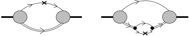
Figure 1: Graphical representation of the function $f_{q/N}(z)$ of Eq.(2.13) in the quark-diquark model. The single (double) line denotes the quark propagator (scalar diquark t-matrix), the hatched circle stands for the quark-diquark vertex function and the operator insertion, denoted by a cross, stands for $\gamma^{+}\delta\left(z-k_{-}/p_{-}\right)$.

The difference with respect to the free nucleon case considered in Ref. [11] is that all propagators have to be replaced by those including the scalar and vector mean fields. The effect of the scalar field can easily be incorporated into the effective masses, but the effect of the vector field is a bit more subtle. In this Subsection we wish to determine this dependence on the vector field more generally, without explicit reference to Feynman diagrams.

For this purpose, we note the following two points. First, the quark field satisfies

$$\psi(w)=e^{i{\hat{P}}_{q}\cdot w}\psi(0)e^{-i{\hat{P}}_{q}\cdot w}\,,$$ (2.15)

where ${\hat{P}}_{q}^{\mu}=({\hat{H}}_{q},{\hat{\mbox{\boldmath${P}$}}}_{q})$ the 4-momentum operator for quarks. The dependence of the quark Hamiltonian on the vector field has been given in Eq. (2.6). Since $[\hat{h}_{q},\hat{Q}]=0$ and $\hat{Q}$ is time independent, we have

$$\frac{\partial\psi(w)}{\partial V_{0}}=iw^{0}[{\hat{Q}},\psi(w)]=-iw^{0}\psi(w),$$

the solution of which can be written in the form of a local gauge transformation :

$$\psi(w)=e^{-iV\cdot w}\psi_{0}(w).$$ (2.16)

Here $\psi_{0}$ is the quark field in the absence of the vector potential.

Second, if the nucleon state $|N,p\rangle$ is an eigenstate of the quark Hamiltonian, ${\hat{H}}_{q}$, with eigenvalue $p^{0}$ given by Eq.(2.5), and of the quark number operator ${\hat{Q}}$ with eigenvalue $3$, it is also an eigenstate of ${\hat{h}}_{q}$ with eigenvalue $p_{\rm N}^{0}$, which is related to $p^{0}$ by Eq.(2.7). We can express this fact in the following way:

$$|N,p\rangle=|N,p_{\rm N}\rangle_{0}\,,$$ (2.17)

where the subscript $0$ characterizes a nucleon state without the external vector field, which we normalize in the same way as Eq. (2.11). If we insert the relations (2.16) and (2.17) into Eq.(2.9), we obtain

$$f_{q/N}(z)=\frac{p_{-}}{p_{{\rm N}-}}\,f_{q/N0}(z^{\prime}\equiv\frac{p_{-}}{p_{{\rm N}-}}z-\frac{V_{-}}{p_{{\rm N}-}})\,,$$ (2.18)

where $f_{q/N0}(z^{\prime})$ is the distribution function in the absence of the vector potential and can simply be evaluated by following the method for the free nucleon case [11] with modified masses. Since in our valence quark picture (no sea quarks) the function $f_{q/N0}(z^{\prime})$ has support for $0<z^{\prime}<1$ [11, 21], the distribution $f_{q/N}(z)$ has support in the region $R_{N}(z)$ defined by

$$R_{N}(z):\,\,\,\,\,\,\,\,\,\,\,\,\,\,\,\,\,\,\,\,\frac{V_{-}}{p_{-}}<z<1-\frac{2V_{-}}{p_{-}}\,\,\,\,\,\,\,\,\,\,\,\,\,\,\,({\rm support}\,\,{\rm of}\,\,f_{q/N}(z))\,.$$ (2.19)

Here we make several comments. First, in the quark-diquark model, the result (2.18) also follows from a straightforward calculation of the Feynman diagrams of Fig.1 – as shown in Appendix A. Second, this discussion concerning the dependence on the vector field can easily be generalized to any hadron (H) with quark number $H$. This leads to

$$f_{q/H}(z)=\frac{p_{-}}{p_{{\rm H}-}}\,f_{q/H0}(z^{\prime}\equiv\frac{p_{-}}{p_{{\rm H}-}}z-\frac{V_{-}}{p_{{\rm H}-}})\,,$$ (2.20)

where $p^{\mu}$ is the momentum of the hadron and

$$p_{\rm H}^{\mu}=p^{\mu}-H\,V^{\mu}$$ (2.21)

is its kinetic momentum. The distribution (2.20) has support in the region $R_{H}(z)$ defined by

$$R_{H}(z):\,\,\,\,\,\,\,\,\,\,\,\,\,\,\,\,\,\,\,\,\frac{V_{-}}{p_{-}}<z<1-\frac{(H-1)V_{-}}{p_{-}}\,\,\,\,\,\,\,\,\,\,\,\,\,\,\,({\rm support}\,\,{\rm of}\,\,f_{q/H}(z))\,.$$ (2.22)

The quark number, $H=3$, corresponds to the case of the nucleon (H=N), which was discussed above. Third, the relation (2.18) shows that $f_{q/N}(z)$ actually depends not only on $z$, but also on $p_{-}$, or on $y_{A}$ (since $y_{A}=Ap_{-}/P_{-}$), although we do not indicate this fact explicitly in our notation. This dependence on the nucleon momentum, which arises because in the medium there is no Lorentz invariance with respect to the motion of a single nucleon, has to be taken into account in the convolution integral (2.8), as will be discussed in Sect.3. Fourth, in Appendix B we show the consistency of (2.22) with the spectral representation

$$f_{q/H}(z)=p_{-}\,\sqrt{2}\sum_{n}\delta(p_{-}(1-z)-p^{(n)}_{-})\,\,|\langle n|\psi_{(+)}|H,p\rangle|^{2}\,,$$ (2.23)

where $\psi_{(+)}=\Lambda_{+}\,\psi$ with $\Lambda_{+}=\gamma^{0}\gamma^{+}/\sqrt{2}$. That is, following the discussions in Ref.[21], there are contributions from connected and semi-connected diagrams to the r.h.s. of Eq.(2.23) and the connected piece (diagram 1 of Fig. 8 in Appendix B) has support only in the region (2.22), while the semi-connected pieces have support in different regions of $z$. The connected piece can be interpreted as the LC momentum distribution of quarks in the hadron H in the sense of the parton model.

If we suppose that the distribution $f_{q/H0}(z)$ satisfies the number and momentum sum rules, which is the case in the quark-diquark model for the nucleon ($H=N$) [11], Eq.(2.20) can be used to confirm the validity of these sum rules for $f_{q/H}(z)$:

$$\int_{R_{H}}{\rm d}z\,f_{q/H}(z) = \int_{0}^{1}{\rm d}z^{\prime}\,f_{q/H0}(z^{\prime})=H\,,$$ (2.24)

$$\int_{R_{H}}{\rm d}z\,z\,f_{q/H}(z) = \frac{p_{{\rm H}-}}{p_{-}}\int_{0}^{1}{\rm d}z^{\prime}\,z^{\prime}\,f_{q/H0}(z^{\prime})+\frac{V_{-}}{p_{-}}\int_{0}^{1}{\rm d}z^{\prime}\,f_{q/H0}(z^{\prime})$$ (2.25)

$$= \frac{p_{{\rm H}-}}{p_{-}}+\frac{HV_{-}}{p_{-}}=1\,.$$

This derivation clearly shows that the shift of the momentum fraction induced by the vector potential (see Eq.(2.20)) is necessary to satisfy the number and momentum sum rules at the same time.

2.2 Nucleon LC momentum distribution in nuclear matter

The function $f_{N/A}(y_{A})$ of Eq.(LABEL:fna) has been discussed in detail in Ref.[6] for the case of a mean field description of NM and we briefly summarize the derivation here for convenience. First we express (LABEL:fna) as follows:

$$f_{N/A}(y_{A})=\frac{-i}{A}\int\frac{{\rm d}^{4}p}{(2\pi)^{4}}\,\delta\left(y_{A}-\frac{\sqrt{2}p_{-}}{\overline{M}_{N}}\right)\,{\rm tr}\left(\gamma^{+}G_{N}(p)\right)\,,$$ (2.26)

where we used Eq.(2.2) and introduced the nucleon two-point function in the medium

$$G_{N,\beta\alpha}(p)=i\int{\rm d}^{4}w\,e^{ip\cdot w}\,\langle A,P|T\,\left[\overline{\psi}_{N,\alpha}(0)\,\psi_{N,\beta}(w)\right]|A,P\rangle\,.$$ (2.27)

The relation to the familiar Feynman propagator in the medium $S_{N}(p)$ [22] is given by

$$G_{N}(p)=V\sqrt{2}\,S_{N}(p)\,,$$ (2.28)

where $V$ is the volume of the system. The propagator $S_{N}(p)$ consists of a “Feynman part” $S_{NF}(p)=\left(\mbox{$\!\not\!p$}_{\rm N}-M_{N}+i\epsilon\right)^{-1}$, and a density dependent part, $S_{ND}(p)$, which takes into account the fact that NM consists of nucleons with momenta up to the Fermi momentum $p_{F}$:

$$S_{ND}(p)=\frac{\mbox{$\!\not\!p$}_{\rm N}+M_{N}}{E_{p}}\,i\pi\,\delta\left(p_{{\rm N}0}-E_{p}\right)\,\Theta(p_{F}-|{\mbox{\boldmath${p}$}}|)\,,$$ (2.29)

where the kinetic momentum $p_{\rm N}$ in these expressions was defined in Eq.(2.7). In the mean field description of the NM ground state, we have to replace [22] $S_{N}\rightarrow S_{ND}$ in loop integrals like in Eq.(2.26), which becomes

$$f_{N/A}(y_{A})=\frac{-i\sqrt{2}}{\rho}\int\frac{{\rm d}^{4}p}{(2\pi)^{4}}\,\delta\left(y_{A}-\frac{\sqrt{2}p_{-}}{\epsilon_{F}}\right)\,{\rm tr}\left(\gamma^{+}S_{ND}(p)\right)\,.$$ (2.30)

Here $\rho$ is the baryon density and we used the fact that at the saturation density the mass per nucleon is equivalent to the Fermi energy  that is, using Eq.(2.5),

$$\overline{M}_{N}=\epsilon_{F}=\sqrt{p_{F}^{2}+M_{N}^{2}}+3V_{0}\equiv E_{F}+3V_{0}.$$ (2.31)

The expression (2.30), which is graphically represented by Fig.2, can easily be evaluated with the result

$$f_{N/A}(y_{A})=\frac{3}{4}\left(\frac{\epsilon_{F}}{p_{F}}\right)^{3}\left[\left(\frac{p_{F}}{\epsilon_{F}}\right)^{2}-(1-y_{A})^{2}\right]$$ (2.33)

$$1-\frac{p_{F}}{\epsilon_{F}}<y_{A}<1+\frac{p_{F}}{\epsilon_{F}}.$$

Figure 2: Graphical representation of the function $f_{N/A}(y_{A})$ of Eq.(2.30). The closed line denotes the nucleon propagator $S_{ND}$, and the operator insertion, denoted by a cross, stands for $\gamma^{+}\delta\left(p_{-}-\frac{\epsilon_{F}\,y_{A}}{\sqrt{2}}\right)$.

It is easy to verify that (2.33) satisfies the relation 

$$f_{N/A}(y_{A})=\frac{\epsilon_{F}}{E_{F}}f_{N/A0}\left(y^{\prime}_{A}\equiv\frac{\epsilon_{F}}{E_{F}}y_{A}-\frac{3V_{0}}{E_{F}}\right)\,,$$ (2.34)

where $f_{N/A0}(y^{\prime}_{A})$ is the distribution obtained by setting $V_{0}=0$ in Eqs. (2.33) and (2.33):

$$f_{N/A0}(y^{\prime}_{A})=\frac{3}{4}\left(\frac{E_{F}}{p_{F}}\right)^{3}\left[\left(\frac{p_{F}}{E_{F}}\right)^{2}-(1-y^{\prime}_{A})^{2}\right]$$ (2.36)

$$1-\frac{p_{F}}{E_{F}}<y^{\prime}_{A}<1+\frac{p_{F}}{E_{F}}.$$

The number and momentum sum rules for the nucleons are easily verified by noting that any function of the form ${\displaystyle f(y)=\frac{3}{4}\frac{1}{a^{3}}\left[a^{2}-(1-y)^{2}\right]}$, where $1-a<y<1+a$, satisfies ${\displaystyle\int{\rm d}y\,f(y)=\int{\rm d}y\,y\,f(y)=1}$ for any value of $a$. That is, both $f_{N/A}$ and $f_{N/A0}$ satisfy the baryon number and momentum sum rules

$$\int{\rm d}y_{A}\,f_{N/A}(y_{A}) = \int{\rm d}y_{A}\,y_{A}\,f_{N/A}(y_{A})=1\,,$$ (2.37)

$$\int{\rm d}y^{\prime}_{A}\,f_{N/A0}(y^{\prime}_{A}) = \int{\rm d}y^{\prime}_{A}\,y^{\prime}_{A}\,f_{N/A0}(y^{\prime}_{A})=1\,,$$ (2.38)

where the ranges of integration are given by Eqs. (2.33) and (2.36).

Although the form (2.33) formally satisfies the sum rules for any values of $p_{F}$ and $\epsilon_{F}$, one should keep in mind that it is valid only at the saturation point – since we used the relation (2.31) which follows from the saturation condition. Neither the momentum sum rule, nor the relation (2.34), would hold if one were to take $\overline{M}_{N}$ to be a fixed parameter.

2.3 Quark momentum distribution in nuclear matter

In order to obtain the dependence of the quark LC momentum distributions in NM on the vector field, we have to insert (2.18) and (2.34) into the convolution formula (2.8). As we pointed out already, because of the presence of the mean vector field, which refers to the NM rest frame, $f_{q/N}(z)$ actually depends also on $y_{A}$. Convolution integrals of the type (2.8) are treated generally in Appendix C and the result is as follows:

$$f_{q/A}(x_{A})=\frac{\epsilon_{F}}{E_{F}}f_{q/A0}(x^{\prime}_{A}=\frac{\epsilon_{F}}{E_{F}}x_{A}-\frac{V_{0}}{E_{F}}).$$ (2.39)

Here the distribution without the explicit effect of the mean vector field is denoted by $f_{q/A0}(x^{\prime}_{A})$ and defined as

$$f_{q/A0}(x^{\prime}_{A})=\int{\rm d}y^{\prime}_{A}\int{\rm d}z^{\prime}\,\delta(x^{\prime}_{A}-y^{\prime}_{A}z^{\prime})\,f_{q/N0}(z^{\prime})\,f_{N/A0}(y^{\prime}_{A})\,.$$ (2.40)

The distribution $f_{q/A0}(x^{\prime}_{A})$ includes, besides the Fermi motion of nucleons, only the effect of the scalar field, which is incorporated easily into the effective masses. Because of the constraint $0<z^{\prime}<1$ and the support of $y_{A}^{\prime}$ given in Eq. (2.36), the distribution (2.40) has support for $0<x_{A}^{\prime}<1+p_{F}/E_{F}$ and the distribution (2.39), which includes the effect of the mean vector field, has support in the region

$$R_{A}(x_{A}):\,\,\,\,\,\,\,\,\,\,\,\,\,\,\,\,\,\,\,\,\frac{V_{0}}{\epsilon_{F}}<x_{A}<\frac{E_{F}+p_{F}+V_{0}}{\epsilon_{F}}\,\,\,\,\,\,\,\,\,\,\,\,\,\,\,({\rm support}\,\,{\rm of}\,\,f_{q/A}(x_{A}))\,.$$ (2.41)

Since we have already shown the sum rules for $f_{q/N}$ and $f_{N/A}$, the sum rules for $f_{q/A}(x_{A})$ follow immediately from the convolution formula (2.8). One can also make direct use of Eq. (2.39) to check the validity of the sum rules, which shows the importance of the shift arising from the mean vector field more explicitly. Indeed, using the fact that the distribution (2.40) satisfies the number and momentum sum rules, we obtain

$$\int_{R_{A}}{\rm d}x_{A}\,f_{q/A}(x_{A}) = \int_{0}^{1+a_{0}}{\rm d}x_{A}^{\prime}\,f_{q/A0}(x_{A}^{\prime})=3\,,$$ (2.42)

$$\int_{R_{A}}{\rm d}x_{A}\,x_{A}\,f_{q/A}(x_{A}) = \frac{E_{F}}{\epsilon_{F}}\int_{0}^{1+a_{0}}{\rm d}x_{A}^{\prime}\,x_{A}^{\prime}\,f_{q/A0}(x_{A}^{\prime})+\frac{V_{0}}{\epsilon_{F}}\int_{0}^{1+a_{0}}{\rm d}x_{A}^{\prime}\,f_{q/A0}(x_{A}^{\prime})$$ (2.43)

$$= \frac{E_{F}}{\epsilon_{F}}+\frac{3V_{0}}{\epsilon_{F}}=1\,,$$

where ${\displaystyle a_{0}=\frac{p_{F}}{E_{F}}}$.

3 Model for the nucleon and nuclear matter

In order to evaluate the quark distributions and structure functions in NM, we need a model for the nucleon and the EOS of NM. In this work, we use the NJL model as an effective quark theory to describe the nucleon as a quark-diquark bound state and NM in the mean field approximation. The details are explained in Refs. [9, 10], and here we will only briefly summarize those points which will be needed for our calculations.

The NJL model is characterized by a chirally symmetric 4-fermi interaction between the quarks. Any such interaction can be Fierz symmetrized and decomposed into various $q\overline{q}$ channels [13]. Writing out explicitly only those channels which are relevant for our present discussion, we have

$${\cal L}={\overline{\psi}}\left(i\mbox{$\!\not\!\partial$}-m\right)\psi+G_{\pi}\left(\left(\overline{\psi}\psi\right)^{2}-\left(\overline{\psi}(\gamma_{5}\mbox{\boldmath${\tau}$})\psi\right)^{2}\right)-G_{\omega}\left(\overline{\psi}\gamma^{\mu}\psi\right)^{2}+\ldots$$ (3.1)

where $m$ is the current quark mass. The quark bilinears $\overline{\psi}\psi$ and $\overline{\psi}\gamma^{\mu}\psi$ have expectation values in the NM ground state $|\rho\rangle$, which we will separate as usual according to $\overline{\psi}\psi=\langle\rho|\overline{\psi}\psi|\rho\rangle+(:\overline{\psi}\psi:)$ and $\overline{\psi}\gamma^{\mu}\psi=\langle\rho|\overline{\psi}\gamma^{\mu}\psi|\rho\rangle+(:\overline{\psi}\gamma^{\mu}\psi:)$. The Lagrangian can then be expressed as

$${\cal L}={\overline{\psi}}\left(i\mbox{$\!\not\!\partial$}-M-\mbox{$\!\not\!V$}\right)\psi-\frac{(M-m)^{2}}{4G_{\pi}}+\frac{V_{\mu}V^{\mu}}{4G_{\omega}}+{\cal L}_{I},$$ (3.2)

where $M=m-2G_{\pi}\langle\rho|\overline{\psi}\psi|\rho\rangle$ and $V^{\mu}=2G_{\omega}\langle\rho|\overline{\psi}\gamma^{\mu}\psi|\rho\rangle$, and ${\cal L}_{I}$ is the normal ordered interaction Lagrangian, including the counter terms linear in the normal ordered products.

In order to fully define the model one has to define a cut-off procedure. In all calculations in this paper we will use the proper time regularization scheme [23, 9], where one evaluates loop integrals over a product of propagators by introducing Feynman parameters, performing the Wick rotation and replacing the denominator ($A$) of the loop integral according to

$$\frac{1}{A^{n}}\rightarrow\frac{1}{(n-1)!}\int_{1/\Lambda_{\rm UV}^{2}}^{1/\Lambda_{\rm IR}^{2}}{\rm d}\tau\,\tau^{n-1}\,e^{-\tau A}\,\,\,\,\,\,\,\,\,(n\geq 1),$$ (3.3)

where $\Lambda_{\rm IR}$ and $\Lambda_{\rm UV}$ are the infrared (IR) and ultraviolet (UV) cut-offs, respectively. Although there are no IR divergences in the theory, the IR cut-off plays the important role of eliminating the imaginary part of the loop integrals. That is, it eliminates the unphysical thresholds for the decay of the nucleon and mesons into quarks [23], thereby taking into consideration a particular aspect of confinement physics. It has been shown in Ref.[9] that this is crucial to describe saturation of the NM binding energy in the NJL model.

3.1 Model for the nucleon

One can use a further Fierz transformation to decompose ${\cal L}_{I}$ into a sum of $qq$ channel interaction terms [13]. For our purposes we need only the interaction in the scalar diquark ($J^{\pi}=0^{+},T=0$, color ${\overline{3}}$) channel:

$${\cal L}_{I,s}=G_{s}\left(\overline{\psi}\left(\gamma_{5}C\right)\tau_{2}\beta^{A}\overline{\psi}^{T}\right)\left(\psi^{T}\left(C^{-1}\gamma_{5}\right)\tau_{2}\beta^{A}\psi\right),$$ (3.4)

where $\beta^{A}=\sqrt{3/2}\,\,\lambda^{A}\,\,(A=2,5,7)$ are the color ${\overline{3}}$ matrices and $C=i\gamma_{2}\gamma_{0}$. The coupling constant $G_{s}$ will be determined so as to reproduce the free nucleon mass.

The reduced t-matrix in the scalar diquark channel is given by [9]

$$\tau(q)=\frac{4iG_{s}}{1+2G_{s}\Pi_{s}(q)}=\tau_{0}(q_{\rm D})$$ (3.5)

with the scalar $qq$ bubble graph

$$\Pi_{s}(q)=6i\int\frac{{\rm d}^{4}k}{(2\pi)^{4}}tr_{D}\left[\gamma_{5}S(k)\gamma_{5}S\left(-(q-k)\right)\right]=\Pi_{s0}(q_{\rm D})\,.$$ (3.6)

In the second equalities of Eqs. (3.5) and (3.6) we indicated that these quantities can be obtained from their expressions without the effect of the mean vector field by replacing $q\rightarrow q_{\rm D}$, where $q_{\rm D}$ is the kinetic momentum of the diquark defined by $H=2$ in (2.21). This is easily seen by using the following form of the quark propagator in the presence of the mean vector field:

$$S(k)=\left(\mbox{$\!\not\!k$}_{\rm Q}-M+i\epsilon\right)^{-1}=S_{0}(k_{\rm Q})\,,$$ (3.7)

where the kinetic momentum of the quark is defined by $H=1$ in (2.21) and $S_{0}$ is the usual Feynman propagator without the effect of the external vector field.

The relativistic Faddeev equation in the NJL model has been solved numerically for the free nucleon in earlier work [13]. For the present purposes, however, because we need to solve the equation many times in order to obtain self-consistency in-medium, we restrict ourselves to the static approximation to the Faddeev equation [24], where the momentum dependence of the quark exchange kernel is neglected. The solution for the quark-diquark t-matrix then takes the simple analytic form

$$T(p)=\frac{3}{M}\frac{1}{1+\frac{3}{M}\Pi_{N}(p)}=T_{0}(p_{\rm N})\,,$$ (3.8)

with the quark-diquark bubble graph given by

$$\Pi_{N}(p)=-\int\frac{{\rm d}^{4}k}{(2\pi)^{4}}\,S(k)\,\tau(p-k)=\Pi_{N0}(p_{\rm N}).$$ (3.9)

In these relations, again, the subscript $0$ characterizes the quantities without the effect of the mean vector field. The nucleon mass $M_{N}$ is defined as the pole of (3.8) at $\mbox{$\!\not\!p$}_{\rm N}=M_{N}$ and the positive energy spectrum has the form given in Eq.(2.5).

The nucleon vertex function in the non-covariant LC normalization is defined by the pole behavior of the quark-diquark t-matrix in the variable $p_{+}\,$:

$$T(p)\rightarrow\frac{\Gamma_{N}(p)\,\overline{\Gamma}_{N}(p)}{p_{+}-\tilde{\epsilon}_{p}}\,\,\,\,\,\,\,\,\,\,\,\,\,\,\,{\rm as}\,\,\,p_{+}\rightarrow\tilde{\epsilon}_{p}\,,$$ (3.10)

where $\tilde{\epsilon}_{p}$ is the “LC energy”. From this definition and Eq.(3.8) one obtains

$$\Gamma_{N}(p)=\sqrt{-Z_{N}\,\frac{M_{N}}{p_{{\rm N}-}}}\,\,u_{N}(p_{\rm N})\,,$$ (3.11)

where $u_{N}$ is a free Dirac spinor for mass $M_{N}$ normalized as $\overline{u}_{N}u_{N}=1$ and for an on-shell nucleon we have $p_{{\rm N}-}=(E_{p}-p_{3})/\sqrt{2}$. The normalization factor $Z_{N}$ is given by

$$Z_{N}=\left[\left(-\frac{\partial\Pi_{N0}(p)}{\partial\mbox{$\!\not\!p$}}\right)_{\mbox{$\!\not\!p$}=M_{N}}\right]^{-1}\,.$$ (3.12)

We note that in this normalization the vertex function satisfies the relation

$$\overline{\Gamma}_{N}(p)\,\left(\frac{\partial\Pi_{N0}(p)}{\partial p_{+}}\right)\,\Gamma_{N}(p)=1.$$ (3.13)

In the numerical calculations of this paper, we will approximate the quantity $\tau_{0}$ by

$$\tau_{0}(q)\rightarrow 4iG_{s}-\frac{i\,g_{D}}{q^{2}-M_{D}^{2}}.$$ (3.14)

Here the diquark mass $M_{D}$ is the pole of $\tau_{0}$ of Eq.(3.5) and the residue is given by

$$g_{D}=2\left[\left(-\frac{\partial\Pi_{s0}(q)}{\partial q^{2}}\right)_{q^{2}=M_{D}^{2}}\right]^{-1}\,.$$ (3.15)

3.2 Evaluation of quark distributions via the moments

The calculation of the distribution $f_{q/N0}$, which appears in the convolution integral (2.40), in the quark-diquark model follows the lines explained in Ref.[11] for the free nucleon. The difference, however, is that here we are using the proper time regularization scheme, which is defined in the Euclidean formulation after Wick rotation. In this case, the regularized LC momentum distribution cannot be calculated directly from the Feynman diagrams of Fig.1, since in the loop integrals one has to fix the minus component of the quark momentum to a real value, see Eq.(2.13), which is not possible in the Euclidean formulation. We therefore consider first the moments

$$A_{n}=\int_{0}^{1}{\rm d}x\,x^{n-1}\,f_{q/N0}(x)\,,$$ (3.16)

and then derive an expression for the quark distributions which can easily be used in Euclidean regularization schemes.

In the following, we will outline the calculations for the “quark diagram” (first diagram of Fig. 1) and the “diquark diagram” (second diagram of Fig. 1) separately, leaving the details to Appendix D . The contribution from the quark (diquark) diagram will be denoted as $f_{q/N0}^{(Q)}(x)$ ($f_{q/N0}^{(D)}(x)$) and the total isoscalar quark distribution in the nucleon is then given by the sum

$$f_{q/N0}(x)=f_{q/N0}^{(Q)}(x)+f_{q/N0}^{(D)}(x)\,.$$ (3.17)

Here, as in the previous subsection, the subindex ($0$) indicates that the effect of the mean vector field is not included. The contribution of the quark diagram to the n-th moment of $f_{q/N0}(x)$ is given by 

$$A_{n}^{(Q)}=-\overline{\Gamma}_{N}(p)\frac{\partial}{\partial p_{+}}\left(\int\frac{{\rm d}^{4}k}{(2\pi)^{4}}\,\left(\frac{k_{-}}{p_{-}}\right)^{n-1}\,S_{0}(k)\,\,\tau_{0}(p-k)\right)\Gamma_{N}(p).$$ (3.18)

From (3.13) and (3.9) it follows that the contribution of the quark diagram to the first moment (quark number) is equal to $1$.

Because of the derivative in (3.18), only the pole term in the expression (3.14) for $\tau_{0}$ contributes. Introducing a Feynman parameter ($\alpha$), and observing that $g^{--}=0$, we obtain (see Appendix D)

$$A_{n}^{(Q)}=-ig_{D}\,Z_{N}\,\frac{\partial}{\partial\mbox{$\!\not\!p$}}\,\int\frac{{\rm d}^{4}k}{(2\pi)^{4}}\,\int_{0}^{1}{\rm d}\alpha\,\alpha^{n-1}\frac{\left(\mbox{$\!\not\!p$}\alpha+M\right)+\frac{n-1}{2\alpha M_{N}}\left(k_{0}^{2}-k_{3}^{2}\right)}{\left(k^{2}-A(\alpha,p^{2})\right)^{2}}\,,$$

(3.19)

where for the calculation of the derivative it is understood that $p^{2}=\mbox{$\!\not\!p$}^{2}$ and at the end one sets $\mbox{$\!\not\!p$}=M_{N}$. The quantity $A(\alpha,p^{2})$ is defined as

$$A(\alpha,p^{2})=M^{2}(1-\alpha)+M_{D}^{2}\alpha-p^{2}\alpha(1-\alpha)\,.$$ (3.20)

From (3.12) we obtain the following form of the normalization factor $Z_{N}$:

$$Z_{N}^{-1}=-ig_{D}\,\frac{\partial}{\partial\mbox{$\!\not\!p$}}\,\int\frac{{\rm d}^{4}k}{(2\pi)^{4}}\,\int_{0}^{1}{\rm d}\alpha\,\frac{\left(\mbox{$\!\not\!p$}\alpha+M\right)}{\left(k^{2}-A(\alpha,p^{2})\right)^{2}}\,,$$ (3.21)

and from Eqs. (3.19), (3.21) we see that $A_{1}^{(Q)}=1$.

If we perform a partial integration in $\alpha$ for the term $\propto n-1$ in Eq.(3.19) and compare the resulting expression to the definition of the moments (Eq.(3.16)), we can directly read off the distribution function:

$$f_{q/N0}^{(Q)}(x)=-i\,g_{D}\,Z_{N}\,\frac{\partial}{\partial\mbox{$\!\not\!p$}}\,\int\frac{{\rm d}^{4}k}{(2\pi)^{4}}\,\left(\mbox{$\!\not\!p$}x+M-\frac{k_{0}^{2}-k_{3}^{2}}{2M_{N}}\frac{\rm d}{{\rm d}x}\right)\frac{1}{\left(k^{2}-A(x,p^{2})\right)^{2}}$$

(3.22)

for $0<x<1$ and zero otherwise. This expression can readily be used in Euclidean regularization schemes. Performing a Wick rotation and introducing the proper time regularization scheme (3.3), we finally obtain

$$f_{q/N0}^{(Q)}(x)=\frac{g_{D}\,Z_{N}}{16\pi^{2}}(1-x)\int_{1/\Lambda_{\rm UV}^{2}}^{1/\Lambda_{\rm IR}^{2}}\frac{{\rm d}\tau}{\tau}e^{-\tau A(x,M_{N}^{2})}\left[1+\tau x\left(\left(M_{N}+M\right)^{2}-M_{D}^{2}\right)\right]\,.$$

(3.23)

The contribution of the diquark diagram of Fig.1 to the distribution $f_{q/N0}$ can be expressed as a convolution integral, involving the quark distribution in a virtual diquark ($f_{q/D0}$) and the diquark distribution in the nucleon ($f_{D/N0}$). For simplicity we use here the on-shell approximation for the diquark distribution, that is, we assume that $f_{D/N0}$ has a sharp peak at the diquark virtuality $q_{0}^{2}=M_{D}^{2}$, so that $f_{q/D0}$ can be replaced by its on-shell value and taken out of the integral over the virtuality. Then we use the relation [11] ${\displaystyle\int{\rm d}q_{0}^{2}\,f_{D/N0}(y,q_{0}^{2})=f_{q/N0}^{(Q)}(1-y)}$, where $f_{q/N0}^{(Q)}$ was evaluated above, see (3.23). The contribution of the diquark diagram is then given by

$$f_{q/N0}^{(D)}(x)=\int_{0}^{1}{\rm d}y\int_{0}^{1}{\rm d}z\,\delta(x-yz)f_{q/D0}(z)\,f_{q/N0}^{(Q)}(1-y)\,.$$ (3.24)

Here $f_{q/N0}^{(Q)}$ is given by Eq.(3.23) and we anticipated the fact that $f_{q/D0}(z)$ has support for $0<z<1$. To evaluate $f_{q/D0}(z)$, we use the moments (see Eq.(3.10) of Ref.[11])

$$A_{n}^{(q/D)}=-6i\,g_{D}\,\frac{\partial}{\partial q^{2}}\int\frac{{\rm d}^{4}k}{(2\pi)^{4}}\left(\frac{k_{-}}{q_{-}}\right)^{n-1}\,{\rm Tr}_{D}\left(\gamma_{5}S_{0}(k)\gamma_{5}S_{0}(k-q)\right)\,,$$ (3.25)

where one has to set $q^{2}=M_{D}^{2}$ at the end.

Before giving the explicit expressions, let us confirm the number and momentum sum rules. From the form of $g_{D}$ given in (3.15), it follows that $A_{1}^{(q/D)}=2$, and because we have already confirmed that the $n=1$ moment of $f_{q/N0}^{(Q)}$ is equal to $1$, the convolution (3.24) shows that the diquark diagram gives a contribution equal to $2$ to the number sum rule. The number sum rule value for the total distribution (3.17) is therefore

$$\int_{0}^{1}{\rm d}x\,f_{q/N0}(x)=3\,.$$ (3.26)

For the momentum sum rule we obtain

$$\int_{0}^{1}{\rm d}x\,x\,f_{q/N0}(x) = \int_{0}^{1}{\rm d}x\,x\,f_{q/N0}^{(Q)}(x)$$

$$+ \left(\int_{0}^{1}{\rm d}y\,y\,f_{q/N0}^{(Q)}(1-y)\right)\cdot\left(\int_{0}^{1}{\rm d}z\,z\,f_{q/D0}(z)\right)\,.$$

Using the fact that $f_{q/D0}(z)$ is symmetric around ${\displaystyle z=\frac{1}{2}}$ and that its $n=1$ moment is equal to $2$, we see that ${\displaystyle\int_{0}^{1}{\rm d}z\,z\,f_{q/D0}(z)=1}$. The momentum sum rule (LABEL:msum1) then becomes

$$\int_{0}^{1}{\rm d}x\,x\,f_{q/N0}(x)=\int_{0}^{1}{\rm d}x\,x\,f_{q/N0}^{(Q)}(x)+\int_{0}^{1}{\rm d}x\,(1-x)\,f_{q/N0}^{(Q)}(x)=1\,.$$ (3.28)

We now continue with the evaluation of (3.25) and the distribution $f_{q/D0}(x)$. By using a Feynman parameter ($\alpha$) and observing that $g^{--}=0$ we obtain (see Appendix D)

$$A_{n}^{(q/D)} = -24i\,g_{D}\,\frac{\partial}{\partial q^{2}}\int\frac{{\rm d}^{4}k}{(2\pi)^{4}}\int_{0}^{1}{\rm d}\alpha\,\alpha^{n-1}$$ (3.29)

$$\times \frac{M^{2}+q^{2}\alpha(1-\alpha)-k^{2}+\frac{n-1}{2\alpha}(1-2\alpha)(k_{0}^{2}-k_{3}^{2})}{\left(k^{2}+q^{2}\alpha(1-\alpha)-M^{2}\right)^{2}}\,.$$

If we perform a partial integration in $\alpha$ for the term $\propto n-1$ in Eq.(3.29) and compare to the definition of the moments (Eq.(3.16), we obtain

$$f_{q/D0}(x) = -24i\,g_{D}\,\frac{\partial}{\partial q^{2}}\int\frac{{\rm d}^{4}k}{(2\pi)^{4}}\left(M^{2}+q^{2}\alpha(1-\alpha)-k^{2}-\frac{k_{0}^{2}-k_{3}^{2}}{2}\frac{\rm d}{{\rm d}x}\left(1-2x\right)\right)$$ (3.30)

$$\times \frac{1}{\left(k^{2}+q^{2}x(1-x)-M^{2}\right)^{2}}\,,$$

where the derivative ${\rm d}/{\rm d}x$ acts on the whole function on its r.h.s. Performing a Wick rotation and introducing the proper time regularization (3.3), we finally obtain

$$f_{q/D0}(x)=\frac{3g_{D}}{4\pi^{2}}\int_{1/\Lambda_{\rm UV}^{2}}^{1/\Lambda_{\rm IR}^{2}}\frac{{\rm d}\tau}{\tau}\,e^{-\tau\left(M^{2}-M_{D}^{2}x(1-x)\right)}\left(1+M_{D}^{2}\tau x(1-x)\right)\,.$$

(3.31)

The results (3.23) and (3.31) are then inserted into the convolution formula (3.24) to give the contribution of the diquark diagram to the quark distribution function.

3.3 Model for nuclear matter

The EOS of NM in the mean field approximation to the NJL model can be derived in a formal way [10] from the quark Lagrangian (3.2) by using hadronization techniques. Equivalently, but more intuitively, one can use the “hybrid model assumption” that the expectation value of any local quark operator, like the quark Hamiltonian density, can be split into the expectation value in the valence quark vacuum $|0\rangle=|\rho=0\rangle$ and an average over the nucleon Fermi sea consisting of correlated valence quarks. The resulting energy density of isospin symmetric NM at rest has the form [9, 10]

$${\cal E}={\cal E}_{V}-\frac{V_{0}^{2}}{4G_{\omega}}+4\int\frac{d^{3}p}{(2\pi)^{3}}\,\Theta\left(p_{F}-|{\mbox{\boldmath${p}$}}|\right)\,\epsilon_{p},$$ (3.32)

where $\epsilon_{p}$ is given by (2.5) and the vacuum contribution (quark loop) is

$${\cal E}_{V}=12i\int\frac{{\rm d}^{4}k}{(2\pi)^{4}}\,{\rm ln}\,\,\frac{k^{2}-M^{2}+i\epsilon}{k^{2}-M_{0}^{2}+i\epsilon}+\frac{(M-m)^{2}}{4G_{\pi}}-\frac{(M_{0}-m)^{2}}{4G_{\pi}}\,.$$ (3.33)

The condition $\partial{\cal E}/\partial V_{0}=0$ leads to

$$V_{0}=6\,G_{\omega}\,\rho\,,$$ (3.34)

and we can eliminate the vector field in (3.32) in favor of the baryon density. The resulting expression has then to be minimized with respect to the constituent quark mass $M$ for fixed density. For zero density this condition becomes identical to the familiar gap equation of the NJL model, and for finite density the nonlinear $M$-dependence of the nucleon mass $M_{N}$, which is obtained from the pole of $T_{0}(p)$ (see Eq.(3.8)), is essential to obtain saturation of the binding energy per nucleon [9].

4 Results and discussions

In this Section we present our numerical results for the quark LC momentum distributions, the structure functions and the EMC effect. The parameters used in the calculation are the same as in Refs. [9, 10]. The IR cut-off $\Lambda_{\rm IR}$ is fixed at 200 MeV, while the values of $m$, $G_{\pi}$ and $\Lambda_{\rm UV}$ are determined so as to reproduce $M_{0}=400$ MeV by the gap equation in the vacuum, $m_{\pi}=140$ MeV from the pole of the t-matrix in the pionic $q\overline{q}$ channel and $f_{\pi}=93$ MeV from the one quark loop diagram for pion decay. The resulting values are $m=16.9$ MeV, $G_{\pi}=19.60$ GeV^-2, and $\Lambda_{\rm UV}=638.5$ MeV. The coupling constant $G_{s}$ of (3.4) is determined so as to reproduce $M_{N0}=940$ MeV as the pole of the quark-diquark t-matrix at zero density (see Eq. (3.8)), which gives the ratio $r_{s}=G_{s}/G_{\pi}=0.508$. Finally, the coupling constant $G_{\omega}$ is determined so that the curve for the NM binding energy per nucleon $(E_{B}/A$) as a function of the density passes through the empirical saturation point ($\rho,E_{B}/A)=(0.16$ fm${}^{-3},\,15$ MeV), which gives the ratio $r_{\omega}=G_{\omega}/G_{\pi}=0.37$. From the pole of the t-matrix in the vector $q\overline{q}$ channel, this value gives an $\omega$ meson mass in vacuum[10] of $827$ MeV, which is larger than the experimental value ($783$ MeV), but is nevertheless reasonable.

We recall from Ref.[9] that, in this simple NJL model, $G_{\omega}$ is the only free parameter for the NM calculation. Therefore, although the binding energy curve passes through the empirical saturation point, its minimum is at a different point, ($\rho,E_{B}/A)=(0.22$ fm${}^{-3},\,17.3$ MeV), see Fig. 6 of Ref.[9]. As we discussed in Sect.2, in the derivation of Eq. (2.39) for the quark distribution in NM we assumed that $\overline{M}_{N}=\epsilon_{F}$, which holds only at the minimum of the binding energy curve. Therefore, although our calculated saturation density $\rho=0.22$ fm^-3 is larger than the empirical one, we have to use this density in our numerical calculations for consistency .

In Table 1 we list the effective quark, diquark and nucleon masses, the vector field acting on the quark ($V_{0}$), the nucleon Fermi energy and the mass per nucleon $\overline{M}_{N}=M_{N0}-E_{B}/A$ at $\rho=0$, $\rho=0.16$ fm^-3, and $\rho=0.22$ fm^-3. We note that for $\rho=0.22$ fm^-3 the sum $M+M_{D}$ is smaller than $M_{N}$, which is possible because of the absence of unphysical thresholds in our regularization procedure.

	$\rho=0$	$\rho=0.16$fm-3	$\rho=0.22$fm-3
$M$	400	308	276
$M_{D}$	576	413	355
$M_{N}$	940	707	634
$V_{0}$	0	53	75
$\epsilon_{F}$	940	914	923
$\overline{M}_{N}$	940	925	923

Table 1: Effective masses $M$, $M_{D}$ and $M_{N}$ for the quark, the diquark and the nucleon, the vector field for quarks ($V_{0}$), the nucleon Fermi energy ($\epsilon_{F}$), and the mass per nucleon $\overline{M}_{N}=M_{N0}-E_{B}/A$ (all in MeV) at $\rho=0$, $\rho=0.16$ fm^-3 and $\rho=0.22$ fm^-3. The saturation density in the present calculation is $\rho=0.22$fm^-3. The values of the quark-diquark coupling constant $g_{D}$ (see Eq.(3.14)) are 18.23, 16.16, and 15.64 for $\rho=0$, $\rho=0.16$ fm^-3, and $\rho=0.22$ fm^-3, respectively.

We first show our results for the valence up and down quark distributions in the free proton in Figs. 3 and 4. They are given by

$$u_{v}(x) = f_{q/N0}^{(Q)}(x)+\frac{1}{2}\,f_{q/N0}^{(D)}(x)\,,$$ (4.1)

$$d_{v}(x) = \frac{1}{2}\,f_{q/N0}^{(D)}(x)\,,$$ (4.2)

where the contributions from the quark diagram (Eq. (3.23)) and the diquark diagram (Eq. (3.24)) refer to the case $\rho=0$ of Table 1.

Figure 3: The valence up quark LC momentum distribution in the free nucleon, multiplied by $x$. The solid line shows the NJL model result ($Q_{0}^{2}=0.16$ GeV²), the dashed line shows the result after the evolution up to $Q^{2}=10$ GeV², and the dotted line shows the empirical parametrization of Ref.[30].

Figure 4: Same as Fig. 3 for the valence down quark.

The solid lines show our NJL model results. We see clearly that $d_{v}(x)$ is softer than $u_{v}(x)$ – that is, the peak position of $d_{v}(x)$ is at smaller values of $x$. This difference comes from the diquark correlations [27, 12], or, in other words, from the difference between the “hard” distribution $f_{q/N0}^{(Q)}$ and the “soft” one $f_{q/N0}^{(D)}$. The total LC momentum fraction carried by the $u$ quarks is $71\%$ and that of the $d$ quark is $29\%$.

In order to make contact to the measured structure functions, we associate the distributions calculated in the NJL model with some low energy scale $Q_{0}$, where a description in terms of quark degrees of freedom alone is expected to be valid. We then perform the evolution according to the Dokshitzer-Gribov-Lipatov-Altarelli-Parisi (DGLAP) equations [28] up to the value of $Q$ where experimental data for DIS and empirical parametrizations of parton distributions are avaliable . Here we fix $Q_{0}=400$ MeV as in our earlier calculations [11, 12], and perform the evolution up to $Q^{2}=10$ GeV². The resulting valence quark distributions are shown by the dashed lines in Figs. 3 and 4 and they are compared with the empirical distributions of Ref.[30] shown by the dotted lines. We see that our calculation reproduces the main features of the empirical distributions. The calculated total LC momentum fractions at $Q^{2}=10$ GeV² are $29\%$ and $12\%$ for the valence $u$ quarks and the valence $d$ quark, respectively, while the rest is carried by the gluons and sea quarks which are generated by the $Q^{2}$ evolution.

We now discuss the modifications of the quark LC momentum distribution at finite density. For this purpose, we first replace the free quark, diquark and nucleon masses by the effective ones given in the last column of Table 1, which gives the distribution $f_{q/N0}$. Then we calculate the convolution with the nucleon LC momentum distribution according to Eq.(2.40) to obtain $f_{q/A0}$. Finally we include the effect of the vector potential through the scale transformation (2.39) to get the total result, $f_{q/A}$. The results are shown in Fig. 5. The dotted line shows isoscalar valence quark distribution for the free nucleon and the dashed line shows the result when all masses are replaced by the effective ones. We see that the distribution becomes somewhat stiffer – i.e., it has more support for large momentum fractions. This can be understood as follows: For large $x$ the spectator quark, which corresponds to the quark diagram of Fig. 1, gives the most important contribution. From the spectral representation (2.23) it follows that the typical LC momentum fraction carried by the spectator quark is $1-M_{D}/M_{N}$ – in agreement with Ref. [27]. Since in our calculation the ratio $M_{D}/M_{N}$ decreases as the density increases (see Table 1), the fraction carried by the spectator quark increases .

Figure 5: Sum of the valence up and down quark LC momentum distributions at the low energy scale ($Q_{0}^{2}=0.16$ GeV²), multiplied by the LC momentum fraction. The dotted line shows the distribution in the free nucleon, the dashed line is obtained by replacing the free masses by the effective ones, the dot-dashed line shows the result of the convolution (2.40), and the solid line is the final result obtained from the scale transformation (2.39). The LC momentum fraction on the horizontal axis generically refers to the proper variable of each distribution, i.e., $x$ for the dotted and dashed lines, and $x_{A}$ for the dot-dashed and solid lines.

The result of the convolution (2.40) with the nucleon momentum distribution is shown by the dot-dashed line in Fig. 5. Because the nucleon momentum distribution $f_{N/A0}(y)$ has a finite width and is symmetric around $y=1$ (see Eq.(2.36)), the result of the convolution shows the familiar effects of Fermi motion. The support extends beyond $x=1$ and, relative to the dashed line, there is a depletion for intermediate values of $x$. However, we have to note two points here. First, since at this stage the effect of the vector field is not yet included, the convolution (2.40) involves the nucleon momentum distribution (2.36) without the explicit effect of the vector potential, and has an appreciably larger width than the “full” distribution (see (2.33) and (2.36)). Therefore, the effect of the Fermi motion, which is seen by comparing the dashed and dot-dashed lines in Fig. 5, is more pronounced than in the calculations of Ref.[6], where the convolution of the quark distribution in a free nucleon with the full $f_{N/A}$ was considered. Second, Fig. 5 clearly shows that the EMC effect cannot be explained by taking into account only the effects of the scalar potential and Fermi motion: in comparison with the dotted line, the dot-dashed line shows an enhancement in the valence quark region ($x\simeq 0.7$) instead of a quenching.

We now come to the discussion of the effect of the mean vector field on the quark distribution function, as expressed by Eq.(2.39) and shown by the solid line in Fig. 5. If we compare the solid line with the dot-dashed line, we see that the effect of the vector field is to squeeze the quark distribution both from the small and large $x$ side, leading to a reduction of the width, a quenching in the valence quark region and an enhancement in the region of smaller $x$. To understand the origin of this effect, we recall the key points which led to the scaling relation (2.39): The presence of the vector field leads to a shift of the quark momentum according to $k^{\mu}=k_{\rm Q}^{\mu}+V^{\mu}$, see Eq.(2.21) for $H=1$, and of the nucleon chemical potential (mass per nucleon) according to $\epsilon_{F}=E_{F}+3V_{0}$, see Eq.(2.31). Then the ratio of the quark LC momentum to the chemical potential without the effect of the vector field (${\displaystyle x_{A}^{\prime}=\frac{k_{{\rm Q}-}}{E_{F}/\sqrt{2}}}$) is related to the one including the effect of the vector field (${\displaystyle x_{A}=\frac{k_{-}}{\epsilon_{F}/\sqrt{2}}}$) by

$$x_{A}^{\prime}=\frac{k_{-}-V_{-}}{E_{F}/\sqrt{2}}=x_{A}\frac{\epsilon_{F}}{E_{F}}-\frac{V_{0}}{E_{F}},$$ (4.3)

which is just the rescaling of the variables expressed in Eq.(2.39). Using (2.31), this linear relationship between $x_{A}^{\prime}$ and $x_{A}$ can also be expressed as

$$x_{A}^{\prime}=x_{A}\left(1+3v\right)-v\,,$$ (4.4)

where $v=V_{0}/E_{F}$. From Eq.(4.4) we see that for ${\displaystyle x_{A}=\frac{1}{3}}$ we also have ${\displaystyle x_{A}^{\prime}=\frac{1}{3}}$ and for ${\displaystyle x_{A}>\frac{1}{3}}$ we have $x_{A}^{\prime}>x_{A}$, while for ${\displaystyle x_{A}<\frac{1}{3}}$ we have $x_{A}^{\prime}<x_{A}$. Thus, if $f_{q/A0}(x_{A})$ has the shape of a typical valence quark distribution with a peak around ${\displaystyle x_{A}=\frac{1}{3}}$, the distribution ${\displaystyle f_{q/A0}(x_{A}^{\prime}=x_{A}\frac{\epsilon_{F}}{E_{F}}-\frac{V_{0}}{E_{F}})}$, viewed as a function of $x_{A}$, will be squeezed from both sides ($x_{A}<1/3$ and $x_{A}>1/3$), with the amount of squeezing being larger for large $x_{A}$. According to (2.39), this distribution is then multiplied by an overall factor ${\displaystyle\frac{\epsilon_{F}}{E_{F}}}$ so as to satisfy the number and momentum sum rules. This mechanism, which is clearly seen by comparing the dot-dashed and the solid curves in Fig. 5 , is largely responsible for the explanation of the EMC effect in a mean field description of NM, where the vector field couples to the quarks inside the nucleons.

If we finally compare the dotted and solid curves of Fig. 5, we observe an enhancement for momentum fractions between $0.2$ and $0.4$, and a depletion for larger $x$, besides the enhancement for $x\rightarrow 1$ arising from the Fermi motion. These features are consistent with the EMC effect.

We next show in Fig. 6 our results for the nuclear structure function per nucleon, calculated for isospin symmetric NM,

$$F_{2A}(x_{A})=\frac{5}{18}\,x_{A}\,f_{q/A}(x_{A})\,,$$ (4.5)

in comparison to the isoscalar structure function of a free nucleon

$$F_{2N}(x)=\frac{1}{2}\left(F_{2p}(x)+F_{2n}(x)\right)=\frac{5}{18}\,x\,f_{q/N0}(x)\,.$$ (4.6)

Figure 6: The solid line shows the structure function per nucleon in symmetric NM given by Eq.(4.5). It is plotted as a function of $x$ by using the relation ${\displaystyle x_{A}=\frac{M_{N0}}{{\overline{M}}_{N}}\,x}$. The dashed line shows the isoscalar free nucleon structure function of Eq. (4.6).

The curves of Fig. 6 were obtained by evolving the quark distributions shown by the solid and dotted lines in Fig. 5 up to $Q^{2}=10$ GeV². In order to plot the nuclear structure function (4.5) as a function of $x$, we used the relation ${\displaystyle x_{A}=\frac{M_{N0}}{\epsilon_{F}}\,x=1.02\,x}$, see Eqs.(2.3), (2.31) and Table 1. Although this “binding effect” is on the level of a few percent, it gives a non-negligible contribution at large $x$. Fig. 6 clearly shows the suppression of the structure function at large $x$ and the enhancement at smaller $x$, which we discussed above for the distribution function at the low energy scale.

From the two curves of Fig. 6, we obtain the ratio between the nuclear and the nucleon structure functions

$$R_{A/N}(x)=\frac{F_{2A}(x_{A})}{F_{2N}(x)}\,,$$ (4.7)

which is shown in Fig. 7. The data points in this figure are the extrapolations of nuclear DIS data to the NM case [32] .

Figure 7: The ratio (4.7) of the nuclear to the nucleon structure function. The data points are the extrapolations of nuclear DIS data to the NM case [32].

We see that the calculation can reproduce the main features of the EMC effect, namely the suppression at large $x$ and the enhancement at smaller $x$. [The fact that in our calculation the saturation density is too large ($\rho=0.22$ fm^-3) leads to an EMC effect that is slightly too strong at large $x$. This is clear if we compare to the results discussed in Appendix E for $\rho=0.16$ fm^-3 – see Fig. 11.]

5 Summary and conclusions

In this paper we have discussed the modifications of the structure function of a nucleon bound in the nuclear medium. For this purpose, we used an effective chiral quark theory which can account for the quark substructure of a single nucleon, as well as for the saturation properties of the NM binding energy. Our description of NM was carried out in the mean field approximation, which is characterized by mean scalar and vector fields coupling to the quarks inside the nucleons. Our aim was to assess the effects which arise from the quark structure of the bound nucleon.

It is well known that the effects of the mean scalar and vector fields on the level of nucleons, including the Fermi motion, cannot explain the EMC effect. We have investigated these medium modifications at the level of the quark structure and our findings can be summarized as follows. The mean scalar field can simply be incorporated into the effective masses and together with the Fermi motion of nucleons it cannot explain the observed reduction of the EMC ratio in the intermediate $x$ region. The vector field, on the other hand, influences the form of the quark LC momentum distributions directly – on top of its indirect influence through the EOS of the system. This direct modification of the quark distribution by the mean vector field is expressed by Eq.(2.39). As our discussion in Sect.4 showed, it plays a key role in explaining the EMC effect, in the framework of a mean field description of NM in terms of quarks. We note that the relation (2.39) includes the combined effect of the mean vector field on the quark momentum distribution in the nucleon and on the nucleon momentum distribution in NM. While the effect of the mean vector field on the nucleon momentum distribution alone tends to cancel the effect of the scalar field [6], its combined effect is appreciable and works in a direction which is consistent with the EMC data. It is therefore crucial to include the quark substructure of the nucleon for the explanation of the EMC effect.

Our findings are reminiscent of the discussions in Ref. [9] (and, of course Refs. [14]), which emphasized the importance of the fact that the mean scalar field couples to the quarks in the nucleon, instead of to the nucleon as a whole, for the stability of the NM ground state in chiral effective quark theories. Concerning the mean vector field, on the other hand, the quark substructure of the nucleon is not essential as long as we consider only the bulk properties of the system. It is essential, however, for the structure functions and the EMC effect, as we have shown in this paper. The further study of the influence of the quark substructure on medium modifications of nucleon properties along these lines is an important aspect of what has come to be called quark nuclear physics.

Acknowledgment

This work was supported by the Grant in Aid for Scientific Research of the Japanese Ministry of Education, Culture, Sports, Science and Technology, Project No. C2-13640298, the Australian Research Council and The University of Adelaide. The authors wish to thank K. Saito, F. Steffens, K. Tsushima and A. Williams for helpful discussions.

Appendices

Appendix A Verification of Eq.(2.18) from Feynman diagrams

In this Appendix we show that the result of an explicit evaluation of the Feynman diagrams shown in Fig.1 satisfies the general relation (2.18).

First we consider the quark diagram of Fig.1, which gives the following contribution to the distribution function (see Eq.(3.7) of Ref.[11]):

$$f_{q/N}^{(Q)}(x)={\overline{\Gamma}}_{N}(p)\left(\frac{\partial}{\partial p_{+}}\Pi_{N}(x,p)\right)\Gamma_{N}(p)$$ (A.1)

with

$$\Pi_{N}(x,p)=-\int\frac{{\rm d}^{4}k}{(2\pi)^{4}}\delta\left(x-\frac{k_{-}}{p_{-}}\right)S(k)\tau(p-k)\,.$$ (A.2)

Here we make use of (see (3.7) and (3.5))

$$S(k)=S_{0}(k_{\rm Q})\,\,;\,\,\,\,\,\,\,\,\,\,\tau(p-k)=\tau_{0}\left((p-k)_{\rm D}\right)=\tau_{0}(p_{\rm N}-k_{\rm Q})\,,$$ (A.3)

where the kinetic momenta are defined as in (2.21) for H=Q, D and N, corresponding to the quark numbers $H=1,\,2,\,3$. If we make a shift $k\rightarrow k+V$ in (A.2), the $\delta$ function becomes

$$\delta\left(x-\frac{k_{-}+V_{-}}{p_{-}}\right)=\frac{p_{-}}{p_{{\rm N}-}}\,\delta\left(x^{\prime}-\frac{k_{-}}{p_{{\rm N}-}}\right)\,,$$ (A.4)

where ${\displaystyle x^{\prime}=\frac{p_{-}}{p_{{\rm N}-}}x-\frac{V_{-}}{p_{{\rm N}-}}}$. By noting that the on-shell value of $p_{\rm N}^{0}$ is $E_{p}$, see Eq.(2.5), and that the nucleon spinor $\Gamma_{N}(p)$ of Eq.(3.11) differs from the one for a free nucleon (quark-diquark bound state) only by the replacement of the free nucleon mass by the effective one, we immediately obtain the relation

$$f_{q/N}^{(Q)}(x)=\frac{p_{-}}{p_{{\rm N}-}}\,f_{q/N0}^{(Q)}(x^{\prime}=\frac{p_{-}}{p_{{\rm N}-}}x-\frac{V_{-}}{p_{{\rm N}-}})\,,$$ (A.5)

where the distribution $f_{q/N0}^{(Q)}(x^{\prime})$ differs from the expression for a free nucleon only by the replacement of the free masses by the effective ones.

In the on-shell approximation for the diquark, to which our actual calculations of Subsect.3.2 refer, the contribution of the diquark diagram of Fig.1 to the quark distribution function has the form [11]

$$f_{q/N}^{(D)}(x)=\int{\rm d}y\,\int{\rm d}z\,\delta(x-yz)f_{q/D}(z)\,f_{D/N}(y)\,,$$ (A.6)

where

$$f_{D/N}(y)=f^{(Q)}_{q/N}(1-y)=\frac{p_{-}}{p_{{\rm N}-}}f_{D/N0}\left(y^{\prime}=\frac{p_{-}}{p_{{\rm N}-}}y-\frac{2V_{-}}{p_{{\rm N}-}}\right)\,.$$ (A.7)

To derive the second equality in (A.7), we used the result (A.5), and $f_{D/N0}(y^{\prime})=f^{(Q)}_{q/N}(1-y^{\prime})$. The quark distribution in an on-shell diquark is given by (cf. Eq. (3.19) of ref.[11])

$$f_{q/D}(z)=\frac{2}{\partial\Pi_{s}(q)/\partial q_{+}}\,\frac{\partial\Pi_{s}(z,q)}{\partial q_{+}}$$ (A.8)

at the on-shell value $q_{\rm D}^{2}=M_{D}^{2}$. Here the scalar bubble graph is given by (3.6), and

$$\Pi_{s}(z,q)=6i\int\frac{{\rm d}^{4}k}{(2\pi)^{4}}\delta\left(z-\frac{k_{-}}{q_{-}}\right){\rm tr}_{D}\left[\gamma_{5}\,S(k)\gamma_{5}\,S(-(q-k))\right]\,.$$ (A.9)

Here we use again the relations $S(k)=S_{0}(k_{\rm Q}),\,S(-(q-k))=S_{0}(-(q-k)_{\rm Q})=S_{0}(k_{\rm Q}-q_{\rm D})$. Then we perform a shift $k\rightarrow k+V$, and rewrite the delta function as

$$\delta\left(z-\frac{k_{-}+V_{-}}{q_{-}}\right)=\frac{q_{-}}{q_{{\rm D}-}}\delta\left(z^{\prime}-\frac{k_{-}}{q_{{\rm D}-}}\right)\,,$$ (A.10)

where ${\displaystyle z^{\prime}\equiv\frac{q_{-}}{q_{{\rm D}-}}z-\frac{V_{-}}{q_{{\rm D}-}}}$. Noting also that $\Pi_{s}(q)=\Pi_{s0}(q_{\rm D})$, we obtain

$$f_{q/D}(z)=\frac{q_{-}}{q_{{\rm D}-}}\,f_{q/D0}\left(z^{\prime}=\frac{q_{-}}{q_{{\rm D}-}}z-\frac{V_{-}}{q_{{\rm D}-}}\right)\,.$$ (A.11)

The distributions (A.7) and (A.11) must then be inserted into the convolution (A.6). Here we must note that, because of the presence of the vector field, the distribution (A.11) actually depends not only on $z$, but only on $q_{-}$, or on $y$ (since $y=q_{-}/p_{-}$). Convolution integrals of this type are treated generally in Appendix C, and here we have a special case of (C.1) for $h=D$ and $H=N$. Therefore we can immediately read off the result from (C.11):

$$f_{q/N}^{(D)}(x)=\frac{p_{-}}{p_{{\rm N}-}}\,f_{q/N0}^{(D)}(x^{\prime}=\frac{p_{-}}{p_{{\rm N}-}}x-\frac{V_{-}}{p_{{\rm N}-}})\,,$$ (A.12)

where the distribution $f_{q/N0}^{(D)}(x^{\prime})$ differs from the free nucleon expression only by the replacement of the free masses by the effective ones. The sum of (A.5) and (A.12) then reproduces the more general relation (2.18) of the main text.

Appendix B Spectral representations of LC momentum distributions

In this Appendix we show that the support of $f_{q/H}(z)$ given by Eq.(2.22) is consistent with the spectral representation (2.23). Following the discussion of Ref.[21], the contributions to the spectral sum on the r.h.s. of (2.23) can be represented by the four diagrams of Fig.8 .

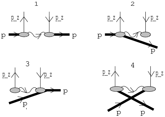
Figure 8: Diagrammatic representation of the r.h.s. of the spectral representation (2.23). The bold line denotes the external hadron H, the thin line a quark, and the wavy line the intermediate state.

In all four diagrams, we have from (2.23)

$$p_{-}^{(n)}=p_{-}(1-z)\,.$$ (B.1)

In the following we discuss the support from these diagrams separately:

1. Diagram 1: The intermediate state $|n>$ has quark number $(H-1)$, where $H$ is the quark number of the initial hadron H. Because the minus component of the kinetic momentum must be positive definite, we obtain

   $$p_{-}^{(n)}-(H-1)V_{-}=p_{-}(1-z)-(H-1)V_{-}>0\,,$$

   which gives the support

   $$z<1-\frac{(H-1)V_{-}}{p_{-}}\,\,\,\,\,\,\,\,\,\,({\rm diagram}\,\,1)\,.$$ (B.2)

2. Diagrams 2 and 3: The intermediate state is $|n>=|n^{\prime}>\otimes|H,p>$, where $|n^{\prime}>$ is indicated by the wavy line in the diagrams, and has quark number $-1$ and minus momentum component given by

   $$p_{-}^{(n^{\prime})}=p_{-}^{(n)}-p_{-}=-p_{-}\,z\,,$$ (B.3)

   where we used (B.1) in the second step. Since the minus component of the kinetic momentum of the state $|n^{\prime}>$ must be positive definite, we obtain

   $$p_{-}^{(n^{\prime})}+V_{-}=-p_{-}\,z+V_{-}>0\,,$$

   which gives the support

   $$z<\frac{V_{-}}{p_{-}}\,\,\,\,\,\,\,\,\,\,({\rm diagrams}\,\,2\,\,{\rm and}\,\,3)\,.$$ (B.4)

3. Diagram 4: The intermediate state is $|n>=|n^{\prime}>\otimes|H,p>\otimes|H,p>$, where $|n^{\prime}>$ is indicated by the wavy line in the diagram, and has quark number $-(H+1)$ and minus momentum component given by

   $$p_{-}^{(n^{\prime})}=p_{-}^{(n)}-2p_{-}=-p_{-}\,(1+z)$$ (B.5)

   where we used (B.1) in the second step. Since the minus component of the kinetic momentum of the state $|n^{\prime}>$ must be positive definite, we obtain

   $$p_{-}^{(n^{\prime})}+(H+1)\,V_{-}=-p_{-}\,(1+z)+(H+1)V_{-}>0\,,$$

   which gives the support

   $$z<-1+\frac{(H+1)V_{-}}{p_{-}}\,\,\,\,\,\,\,\,\,\,({\rm diagram}\,\,4)$$ (B.6)

We therefore see that in the region

$$\frac{V_{-}}{p_{-}}<z<1-\frac{(H-1)V_{-}}{p_{-}}$$ (B.7)

only diagram 1 contributes. Since diagram 1 corresponds to the “quark distribution” in the parton model sense, we obtain the support as given by Eq. (2.19).

Appendix C Convolution integrals

Here we consider convolution integrals of the form

$$f_{q/H}(x)=\int{\rm d}y\int{\rm d}z\,\delta(x-yz)\,f_{q/h}(z)\,f_{h/H}(y)\,,$$ (C.1)

where the distributions refer to hadrons H and h with quark numbers $H$ and $h$, respectively, and the dependence on the mean vector field is expressed as

$$f_{h/H}(y) = \frac{P_{-}}{P_{{\rm H}-}}\,f_{h/H0}\left(y^{\prime}=\frac{P_{-}}{P_{{\rm H}-}}y-\frac{hV_{-}}{P_{{\rm H}-}}\right)$$ (C.2)

$$f_{q/h}(z) = \frac{p_{-}}{p_{{\rm h}-}}\,f_{q/h0}\left(z^{\prime}=\frac{p_{-}}{p_{{\rm h}-}}z-\frac{V_{-}}{p_{{\rm h}-}}\right)\,.$$ (C.3)

The minus momentum components of the hadronic states H and h are $P_{-}$ and $p_{-}$, respectively, and their kinetic momenta are defined as in (2.7). For the case of the convolution (2.8), which is needed in the main text, we have to identify H=A, h=N, and $P_{-}\equiv\epsilon_{F}/\sqrt{2}$, $P_{{\rm H}-}\equiv E_{F}/\sqrt{2}$.

To evaluate (C.1), we make the transformation of variables

$$(y,z) \rightarrow (p_{-},k_{-}),\,\,\,\,\,\,\,\,\,\,{\rm where}$$

$$y \equiv \frac{p_{-}}{P_{-}};\,\,\,\,\,\,\,\,\,\,z\equiv\frac{k_{-}}{p_{-}}\,,$$ (C.4)

and obtain from the Jacobian of this transformation

$${\rm d}y\,{\rm d}z=\frac{1}{P_{-}\,p_{-}}{\rm d}p_{-}\,{\rm d}k_{-}\,.$$ (C.5)

In terms of these variables we have $x=k_{-}/P_{-}$, and the quantities $y^{\prime}$ and $z^{\prime}$ in (C.2) and (C.3) are expressed as

$$y^{\prime}=\frac{p_{{\rm h}-}}{P_{{\rm H}-}}\,\,\,\,\,\,\,\,\,\,\,\,z^{\prime}=\frac{k_{{\rm Q}-}}{p_{{\rm h}-}}\,.$$ (C.6)

Then Eq.(C.1) becomes

$$f_{q/H}(x) = \int{\rm d}k_{-}\int{\rm d}p_{-}\,\delta\left(x-\frac{k_{-}}{P_{-}}\right)\frac{1}{P_{{\rm H}-}\,p_{{\rm h}-}}f_{h/H0}\left(\frac{p_{{\rm h}-}}{P_{{\rm H}-}}\right)\,f_{q/h0}\left(\frac{k_{{\rm Q}-}}{p_{{\rm h}-}}\right)$$ (C.7)

$$= \int{\rm d}k_{{\rm Q}-}\int{\rm d}p_{{\rm h}-}\,\delta\left(x-\frac{k_{{\rm Q}-}+V_{-}}{P_{{\rm H}-}+HV_{-}}\right)\frac{1}{P_{{\rm H}-}\,p_{{\rm h}-}}$$

$$\times f_{h/H0}\left(\frac{p_{{\rm h}-}}{P_{{\rm H}-}}\right)\,f_{q/h0}\left(\frac{k_{{\rm Q}-}}{p_{{\rm h}-}}\right)\,,$$

where we performed a shift $(k_{-},p_{-})\rightarrow(k_{{\rm Q}-},p_{{\rm h}-})$ in the second step. We then introduce the variables

$$y^{\prime} = \frac{p_{{\rm h}-}}{P_{{\rm H}-}},\,\,\,\,\,\,\,\,\,\,z^{\prime}=\frac{k_{{\rm Q}-}}{p_{{\rm h}-}}$$

$$\Rightarrow p_{{\rm h}-}=P_{{\rm H}-}\,y^{\prime},\,\,\,\,\,\,\,\,\,\,k_{{\rm Q}-}=P_{{\rm H}-}\,y^{\prime}z^{\prime}$$

$$\Rightarrow \,\delta\left(x-\frac{k_{{\rm Q}-}+V_{-}}{P_{{\rm H}-}+HV_{-}}\right)=\frac{P_{-}}{P_{{\rm H}-}}\,\delta\left(\frac{P_{-}}{P_{{\rm H}-}}x-z^{\prime}y^{\prime}-\frac{V_{-}}{P_{{\rm H}-}}\right)$$

$$\equiv \frac{P_{-}}{P_{{\rm H}-}}\,\delta\left(x^{\prime}-z^{\prime}y^{\prime}\right)\,,$$ (C.9)

where in the last step we defined

$$x^{\prime}\equiv\frac{P_{-}}{P_{{\rm H}-}}x-\frac{V_{-}}{P_{{\rm H}-}}\,.$$ (C.10)

Then we obtain finally

$$f_{q/H}(x) = \frac{P_{-}}{P_{{\rm H}-}}\int{\rm d}y^{\prime}\int{\rm d}z^{\prime}\,\delta(x^{\prime}-y^{\prime}z^{\prime})\,f_{h/H0}(y^{\prime})f_{q/h0}(z^{\prime})$$ (C.11)

$$= \frac{P_{-}}{P_{{\rm H}-}}f_{q/H0}\left(x^{\prime}=\frac{P_{-}}{P_{{\rm H}-}}x-\frac{V_{-}}{P_{{\rm H}-}}\right)\,.$$

Appendix D Moments and distribution functions in the proper time regularization scheme

In this Appendix we derive the quark distribution functions in the absence of the vector field given in Subsect.3.2.

The contribution of the quark diagram of Fig.1 to the moments is given by (3.18), where only the pole term of $\tau_{0}$ (see Eq.(3.14)) contributes. We combine the two denominators by a Feynman parameter $\alpha$, and shift the loop momentum according to $k\rightarrow k+p\alpha$ to obtain

$$A_{n}^{(Q)}=i\,g_{D}\,{\overline{\Gamma}}_{N}(p)\frac{\partial}{\partial p_{+}}\int\frac{{\rm d}^{4}k}{(2\pi)^{4}}\,\int_{0}^{1}{\rm d}\alpha\left(\frac{k_{-}+p_{-}\alpha}{p_{-}}\right)^{n-1}\frac{\mbox{$\!\not\!k$}+\mbox{$\!\not\!p$}\alpha+M}{\left(k^{2}-A(\alpha,p^{2})\right)^{2}}\,\Gamma_{N}(p)\,,$$

where $A(\alpha,p^{2})$ is defined in Eq.(3.20). In general, invariant integration over a function of the form ${\displaystyle f(k^{2})k^{\alpha}k^{\beta}\dots}$ gives a sum of products of contractions $g^{\alpha\beta}\dots$. If we note that $g^{--}=0$, it is easy to see that, in the expansion of $\left(k_{-}+p_{-}\alpha\right)^{n-1}$, all terms $\propto(k_{-})^{m}$ give no contributions if $m\geq 2$. We can therefore replace $\left(k_{-}+p_{-}\alpha\right)^{n-1}\rightarrow\left(p_{-}\alpha\right)^{n-1}+(n-1)k_{-}\left(p_{-}\alpha\right)^{n-2}$. If we further use ${\displaystyle\mbox{$\!\not\!k$}=k_{+}\gamma_{-}+k_{-}\gamma_{+}-{\mbox{\boldmath${k}$}}_{\perp}\cdot{\mbox{\boldmath${\gamma}$}}_{\perp}}$, as well as the form (3.11) of the nucleon spinor, we obtain

$$A_{n}^{(Q)} = -ig_{D}\,Z_{N}\,\frac{M_{N}}{p_{-}}{\overline{u}}_{N}(p)\left[\frac{\partial}{\partial p_{+}}\int\frac{{\rm d}^{4}k}{(2\pi)^{4}}\,\int_{0}^{1}{\rm d}\alpha\,\alpha^{n-1}\right.$$

$$\times \left.\frac{\alpha\mbox{$\!\not\!p$}+M+\frac{n-1}{2\alpha p_{-}}\left(k_{0}^{2}-k_{3}^{2}\right)\,\gamma_{-}}{\left(k^{2}-A(\alpha,p^{2})\right)^{2}}\right]u_{N}(p)\,.$$

By using the Dirac equation, we can replace $\gamma_{-}\rightarrow p_{-}/M_{N}$ in the last term of the above expression. Because of $p^{2}={\mbox{$\!\not\!p$}}^{2}$, the integrand can then be considered as a function $F({\mbox{$\!\not\!p$}})$, and by noting that

$$\frac{M_{N}}{p_{-}}\overline{u}_{N}(p)\left(\frac{\partial}{\partial p_{+}}\,F(\mbox{$\!\not\!p$})\right)u_{N}(p)=\left(\frac{\partial F}{\partial{\mbox{$\!\not\!p$}}}\right)_{\mbox{$\!\not\!p$}=M_{N}}$$

we arrive at the form (3.19) given in the main text. If we perform a partial integration in $\alpha$ and note that the surface term is independent of $\!\not\!p$, we obtain the expression (3.22) for the distribution function.

We perform a Wick rotation in (3.22), and note that in any $O(4)$ invariant Euclidean regularization scheme we can replace $k_{0}^{2}+k_{3}^{2}\rightarrow k^{2}/2$, where now our notation refers to Euclidean metric ($k^{2}=k_{0}^{2}+{\mbox{\boldmath${k}$}}^{2}$). By introducing the proper time regularization scheme (3.3), we obtain

$$f_{q/N0}^{(Q)}(x)=g_{D}\,Z_{N}\,\frac{\partial}{\partial{\mbox{$\!\not\!p$}}}\int\frac{{\rm d}^{4}k}{(2\pi)^{4}}\,\int_{1/\Lambda_{\rm UV}^{2}}^{1/\Lambda_{\rm IR}^{2}}\,\tau\,{\rm d}\tau\,\left(\mbox{$\!\not\!p$}x+M+\frac{k^{2}}{4M_{N}}\frac{\rm d}{{\rm d}x}\right)e^{-\tau\left(k^{2}+A(x,p^{2})\right)}$$

It is then easy to perform the loop integral and the required derivatives to arrive at the result (3.23) of the main text.

Next we consider the quark LC momentum distribution in the diquark. The moments are given by Eq.(3.25). We calculate the Dirac trace, introduce a Feynman parameter $\alpha$, and shift the loop momentum according to $k\rightarrow k+q\alpha$ to obtain

$$A_{n}^{(q/D)} = -24i\,g_{D}\,\frac{\partial}{\partial q^{2}}\int\frac{{\rm d}^{4}k}{(2\pi)^{4}}\int_{0}^{1}{\rm d}\alpha\,\left(\frac{k_{-}+q_{-}\alpha}{q_{-}}\right)^{n-1}$$

$$\times \frac{M^{2}+q^{2}\alpha(1-\alpha)-k^{2}+k\cdot q(1-2\alpha)}{\left(k^{2}+q^{2}\alpha(1-\alpha)-M^{2}\right)^{2}}\,,$$

where one has to set $q^{2}=M_{D}^{2}$ at the end. Following the same argument as given above for the quark diagram, there are no contributions from $(k_{-})^{m}\,\,(m\geq 2)$ in the expansion of $(k_{-}+q_{-}\alpha)^{n-1}$ because of $g^{--}=0$. By using $k\cdot q=k_{+}q_{+}+k_{-}q_{-}-{\mbox{\boldmath${k}$}}_{\perp}\cdot{\mbox{\boldmath${q}$}}_{\perp}$, we obtain the expression (3.29) of the main text. Performing a partial integration in $\alpha$ and noting that the surface term is independent of $q^{2}$ leads to the distribution function (3.30). We then perform a Wick rotation in (3.30), and note again that in any $O(4)$ invariant Euclidean regularization scheme we can replace $k_{0}^{2}+k_{3}^{2}\rightarrow k^{2}/2$, where now $k^{2}=k_{0}^{2}+{\mbox{\boldmath${k}$}}^{2}$. By introducing the proper time regularization scheme (3.3), we obtain

$$f_{q/D0}(x) = 24\,g_{D}\,\frac{\partial}{\partial q^{2}}\int\frac{{\rm d}^{4}k}{(2\pi)^{4}}\int_{1/\Lambda_{\rm UV}^{2}}^{1/\Lambda_{\rm IR}^{2}}\,{\rm d}\tau$$

$$\times \left(1+2q^{2}x(1-x)\tau+\frac{k^{2}\tau}{4}\frac{\rm d}{{\rm d}x}(1-2x)\right)e^{-\tau\left(k^{2}+M^{2}-q^{2}x(1-x)\right)}\,,$$

where the derivative ${\rm d}/{\rm d}x$ acts on the whole function on its r.h.s. It is then easy to perform the loop integral and the required derivatives to arrive at the result (3.31) of the main text.

Appendix E Results for the case ${\mbox{\boldmath${\rho}$}=}$0.16 fm^-3

The numerical calculations discussed in Sect.4 were performed at the saturation density in our model ($\rho=0.22$ fm^-3), which is too high compared to the empirical value. In order to indicate the dependence on the density, we will show the results for $\rho=0.16$ fm^-3 in this Appendix, using the effective masses and energies listed in Table 1. One should keep in mind, however, that in the derivations of the main text, for example of Eqs.(2.34) and (2.39), the relation ${\overline{M}}_{N}=\epsilon_{F}$ was assumed. As this is satisfied only at the saturation density (see Table 1), the results shown in this Appendix should serve only to indicate qualitatively the density dependence of the results.

Fig.9 shows how the results of Fig. 5 change if we decrease the density to $\rho=0.16$ fm^-3.

Figure 9: Same as Fig.5 for the density $\rho=0.16$ fm^-3.

We see that the various medium modifications of the quark distribution function show a very similar behavior, but their magnitudes are smaller because of the smaller density. The structure function per nucleon in nuclear matter (see Eq.(4.5)) is compared to the free nucleon structure function in Fig. 10. In order to plot the function (4.5) against $x$, we used the relation (2.3) with ${\overline{M}}_{N}$ equal to the mass per nucleon at the density $\rho=0.16$ fm^-3 given in Table 1.

Figure 10: Same as Fig.6 for the density $\rho=0.16$ fm^-3.

The qualitative behavior is the same as in Fig. 6, but the difference between the dashed and solid lines is smaller. Finally, the ratio (4.7) is shown in Fig.11. Compared to Fig.7, the magnitude of the EMC effect is reduced.

Figure 11: Same as Fig.7 for the density $\rho=0.16$ fm^-3.

References

• [1] J. Aubert et al., Phys. Lett. B 123 (1982) 275;
A. Bodek et al., Phys. Rev. Lett. 51 (1983) 534;
R.G. Arnold et al., Phys. Rev. Lett. 52 (1984) 727.
• [2] M. Arneodo, Phys. Rep. 240 (1994) 240;
D.F. Geesaman, K. Saito and A.W. Thomas, Ann. Rev. Nucl. Part. Sci. 45 (1995) 337;
G. Piller and W. Weise, Phys. Rep. 330 (2000) 1.
• [3] S. Strauch et al., Phys. Rev. Lett. 91 (2003) 052301;
D.H. Lu, K. Tsushima, A.W. Thomas, A.G. Williams and K. Saito, Phys. Lett. 417 (1998) 217; Phys. Rev. C 60 (1999) 068201.
• [4] J. G. Messchendorp et al., Phys. Rev. Lett. 89 (2002) 222302;
Z. Aouissat, Nucl. Phys. A 721 (2003) 76c.
• [5] R.L. Jaffe, in Proceedings of the 1985 Los Alamos School on Relativistic Dynamics and Quark Nuclear Physics, edited by M.B. Johnson and A. Pickleseimer (Wiley, New York, 1985).
• [6] G.A. Miller and J. R. Smith, Phys. Rev. C 65 (2002) 015211.
• [7] A. W. Thomas, A. Michels, A. W. Schreiber and P. A. M. Guichon, Phys. Lett. B 233 (1989) 43.
• [8] Y. Nambu and G. Jona-Lasinio, Phys. Rev. 122 (1960) 345; 124 (1961) 246.
• [9] W. Bentz and A.W. Thomas, Nucl. Phys. A 696 (2001) 138.
• [10] W. Bentz, T. Horikawa, N. Ishii and A.W. Thomas, Nucl. Phys. A 720 (2003) 95.
• [11] H. Mineo, W. Bentz and K. Yazaki, Phys. Rev. C 60 (1999) 065201.
• [12] H. Mineo, W. Bentz, N. Ishii and K. Yazaki, Nucl. Phys. A 703 (2002) 785.
• [13] N. Ishii, W. Bentz and K. Yazaki, Nucl. Phys. A 578 (1995) 617;
M. Oettel, R. Alkofer and L. von Smekal, Eur. Phys. J. A 8 (2000) 553.
• [14] P. A. M. Guichon, Phys. Lett. B 200 (1988) 235; P. A. M. Guichon, K. Saito, E. N. Rodionov and A. W. Thomas, Nucl. Phys. A 601 (1996) 349; K. Saito, K. Tsushima and A. W. Thomas, Phys. Rev. C 55 (1997) 2637.
• [15] K. Saito and A.W. Thomas, Nucl. Phys. A 574 (1994) 659.
• [16] A. W. Thomas, Phys. Lett. B 126 (1983) 97.
• [17] M. Ericson and A. W. Thomas, Phys. Lett. B 128 (1983) 112.
• [18] C. H. Llewellyn Smith, Phys. Lett. B 128 (1983) 107.
• [19] M. Ericson and A. W. Thomas, Drell-Yan Process,” Phys. Lett. B 148 (1984) 191.
• [20] D. B. Leinweber, A. W. Thomas and R. D. Young, Phys. Rev. Lett.  86 (2001) 5011.
• [21] R.L. Jaffe, Nucl. Phys. B 229 (1983) 205.
• [22] B.D. Serot and J.D. Walecka, Adv. Nucl. Phys. 11 (1986) 1.
• [23] D. Ebert, T. Feldmann and H. Reinhardt, Phys. Lett. 388 (1996) 154;
G. Hellstern, R. Alkofer and H. Reinhardt, Nucl. Phys. A 625 (1997) 697.
• [24] A. Buck, R. Alkofer and H. Reinhardt, Phys. Lett. 286 (1992) 29.
• [25] N. Ishii, W. Bentz and K. Yazaki, Phys. Lett. B 301 (1993) 165.
• [26] N. Ishii, nucl-th/0306028.
• [27] F.E. Close and A.W. Thomas, Phys. Lett. B 212 (1988) 227;
A.W. Thomas, Phys. Lett. B 126 (1983) 97.
• [28] V.N. Gribov and L.N. Lipatov, Sov. J. Nucl. Phys. 15 (1972) 438; 15 (1972) 675;
G. Altarelli and G. Parisi, Nucl. Phys. B 126 (1977) 298;
Yu. L. Dokshitzer, Zh. Eksp. Teor. Fiz. 73 (1977) 1216 [Sov. Phys. JETP 46 (1977) 641].
• [29] M. Miyama and S. Kumano, Comput. Phys. Commun. 94 (1996) 185.
• [30] A.D. Martin, R.G. Roberts, W.J. Stirling and R.S. Thone (MRST2002), Eur. Phys. J. C 28 (2003) 455 (available electronically at: http://durpdg.dur.ac.uk/hepdata/pdf.html).
• [31] W. Bentz et al., Prog. Theor. Phys. Suppl. 151 (2003) 176.
• [32] I. Sick and D. Day, Phys. Lett. B 274 (1992) 16.