Meson-Meson Interactions and Resonances in the ’t Hooft Model

Abstract

We studied meson-meson interactions using the ’t Hooft model, which represents QCD in $1+1$ dimensions and assumes a large number of colors ($N_{c}$). The dominant interactions in this large $N_{c}$ limit are generated by quark exchange. Our results show that QCD in $1+1$ dimensions allows the realization of a constituent-type quark model for the mesons, and generates a scalar “$\sigma$”-like meson-meson resonance, whose effective coupling and mass are determined by the underlying QCD dynamics. These results suggest an interpretation of the lightest scalar mesons as $q\bar{q}q\bar{q}$ systems.

I Introduction

At low energies, systems which are due to, or interact through, the strong nuclear interaction may be described by effective field theories, examples of which are Quantum Hadrodynamics (QHD) Walecka and Chiral Perturbation Theory gary ), or simple constituent quark models Isgur . With more or less phenomenological content, those frameworks are in general very successful, but there are still questions not completely answered.

For instance, whether the nature of the broad $\sigma$ meson corresponds truly to a simple quark structure, or to a resonance in the meson-meson dynamics, or to an unusual quark structure as a meson-glueball combination, or even to some combination of these, is still an open issue. Models of QCD did not yet resolve this question quantitatively. In general for the light scalar mesons, arguments have been advanced for the importance of a $q\bar{q}q\bar{q}$ component Close at short distances, compatible with a dominant meson-meson component at large distances. A very recent lattice calculation Jaffe also indicates that a $q\bar{q}q\bar{q}$ bound state may exist, just below threshold in the non-exotic channel of pseudoscalar-pseudoscalar s-wave scattering.

In this work we apply the ’t Hooft model thooft , a formulation of QCD in 1+1 dimensions and in the large $N_{c}$ limit, to the meson-meson scattering process. The ’t Hooft model has no physical gluons, thus it includes no glueballs. Furthermore, due to the large $N_{c}$ limit, quark exchange dominates gluon exchange and only a finite number of diagrams contribute. Since the finite sum of regular contributing diagrams is unable to produce a pole at real energies, no meson-meson bound states can be produced.

However, while meson-meson bound states are excluded in this framework, complex energy resonant states should still be possible. It is the purpose of this paper to calculate the meson-meson scattering amplitude based on meson-$q\bar{q}$ vertex functions obtained in the ’t Hooft model, and to look for low-lying resonances. As we will show, the ’t Hooft model indeed supports the existence of meson-meson resonances, suggesting the relevance of the $q\bar{q}q\bar{q}$ structure for the light scalar mesons.

A calculation of $\pi-\pi$ forward and backward scattering in the Dyson-Schwinger, Bethe-Salpeter approach and in the rainbow-ladder approximation was presented in Ref. Cotanch . It uses an effective $q\bar{q}$ interaction and incorporates features of QCD. Based on this approach, a scalar meson emerges as a resonance in $\pi-\pi$ scattering. However, the calculation is performed using the Euclidian metric. In our work, while simplifying the problem by working in 1+1 dimensions, we use the Minkowski metric througout.

Clearly, a model in 1+1 dimensions is limited in its scope, and one has to be very cautious when comparing its results to phenomena in the real world. Nevertheless, for kinematic conditions of scattering processes with a negligible component of the momentum transfer in the transverse direction, we may conjecture that the ’t Hooft model, and thus the calculation presented here, has the main features of realistic microscopic QCD, and that its results are valid at least qualitatively.

Section II reviews the model and introduces the calculational framework. Section III presents the input for the description of the meson-meson scattering transition amplitude. Section IV shows the results, and section V presents the conclusions.

II Formalism

II.1 The ‘t Hooft model and the choice of gauge

This work models the meson-meson interaction using the ’t Hooft model. Here we review briefly the dynamics of this model by starting with the corresponding Lagrangian. Subsequently, we write the equations that we solved for the one body (quark propagator) and two body (quark-antiquark bound state) problems.

The QCD Lagrangian is

$${\cal L}=-\frac{1}{4}Tr\left[G^{\mu\nu}G_{\mu\nu}\right]+\bar{q}\left(iD_{\mu}\gamma^{\mu}-m_{0}\right)q\,,$$ (1)

with the notation

$$A^{\mu}= A^{\mu}_{a}\frac{\lambda_{a}}{2}\,,$$

$$G_{\mu\nu}= \partial_{\mu}A_{\nu}-\partial_{\nu}A_{\mu}+i\alpha\left[A_{\mu},A_{\nu}\right]\,,$$

$$D_{\mu}= \partial_{\mu}+i\alpha A_{\mu}\,,$$ (2)

where $A^{\mu}_{a}$ are the gluon fields with the Lorentz index $\mu$ and the color index $a$, the $\lambda_{a}$’s are the generators of the $SU(N)$ color group, $G_{\mu\nu}$ is the field tensor, $q$ is the quark field, $m_{0}$ is the bare quark mass and $\alpha$ is the quark-gluon coupling strength. Following ’t Hooft thooft , the coupling strength $\alpha$ depends on the number of colors in the following way:

$$\alpha=\frac{g}{\sqrt{N_{c}}}\,.$$ (3)

Introducing for an arbitrary two-vector $b$ the light cone variables:

$$b_{+}=\frac{1}{\sqrt{2}}(b^{0}+b^{1})\,,$$

$$b_{-}=\frac{1}{\sqrt{2}}(b^{0}-b^{1})\,,$$ (4)

the scalar product of any two vectors $a$ and $b$ becomes $a_{+}b_{-}+a_{-}b_{+}$, and the derivatives correspond to

$$\partial_{-}= \frac{\partial}{\partial x_{+}}=\frac{1}{\sqrt{2}}(\partial^{0}-\partial^{1})=\frac{1}{\sqrt{2}}(\frac{\partial}{\partial x^{0}}+\frac{\partial}{\partial x^{1}})\,,$$

$$\partial_{+}= \frac{\partial}{\partial x_{+}}=\frac{1}{\sqrt{2}}(\partial^{0}+\partial^{1})=\frac{1}{\sqrt{2}}(\frac{\partial}{\partial x^{0}}-\frac{\partial}{\partial x^{1}})\,.$$ (5)

In the same way, the $+$ and $-$ components of the $\gamma$ matrices are defined. The anticommutation relations read

$$\{\gamma_{-},\gamma_{-}\}=\{\gamma_{+},\gamma_{+}\}=0\,,$$

$$\{\gamma_{+},\gamma_{-}\}=2\,.$$ (6)

In the light cone variables, the nonvanishing components of the field strength tensor are

$$G_{+-}=-G_{-+}=\partial_{+}A_{-}-\partial_{-}A_{+}+i\alpha[A_{-},A_{+}]\,,$$ (7)

so that the free gauge field Lagrangian becomes

$${\cal L}_{free}=\frac{1}{2}G_{+-}^{2}\,.$$ (8)

We choose to work in the light cone gauge, $A_{-}=0$, so that the commutator contained in the field tensor $G_{+-}$ disappears. Moreover, since we consider only two dimensions, we do not have any physical gluonic degrees of freedom. In addition, because of the gauge condition, there is only one degree of freedom left. Consequently, the gluonic field is not a dynamical variable and does not couple to ghosts any longer.

In this parametrization the Lagrangian (1) becomes

$${\cal L}=\frac{1}{2}Tr\left[(\partial_{-}A_{+})^{2}\right]+\bar{q}\left(i\partial_{+}\gamma_{-}+i\partial_{-}\gamma_{+}-\alpha\gamma_{-}A_{+}-m_{0}\right)q\,.$$ (9)

Before quantizing the theory given by this Lagrangian, we calculate the gluonic field. The equation of motion related to this field is

$$(\frac{\partial}{\partial x_{+}})^{2}A_{+}=-\alpha\bar{q}\gamma_{-}q\,.$$ (10)

The solution of Eq. (10) is

$$A_{+}(x_{+},x_{-})=-\alpha\int dy_{+}\bar{q}(y_{+},x_{-})\gamma_{-}q(y_{+},x_{-}){\cal G}(y_{+}-x_{+})\,,$$ (11)

where the Green’s function ${\cal G}$ is given by

$${\cal G}(y_{+}-x_{+})=|y_{+}-x_{+}|+c_{1}(y_{+}-x_{+})+c_{2}\,.$$ (12)

The coefficients $c_{1}$ and $c_{2}$ are free parameters. This means that the gauge condition did not eliminate all the redundant degrees of freedom, just as the Coulomb or Lorentz gauge do not determine uniquely the photon propagator in QED (Gribov ambiguity). We can therefore set the coefficients $c_{1}$ and $c_{2}$ equal to zero in order to simplify our calculations.

The Fourier transform of the Green’s function (12) gives the gluon “propagator”, or more precisely the momentum dependence of the effective quark-quark interaction:

$$D(k)=D(k_{-})=\frac{1}{k_{-}^{2}}-\delta{(k_{-})}{\cal P}\int_{-\infty}^{\infty}\frac{d\ell_{-}}{\ell^{2}_{-}}\,.$$ (13)

The second term in Eq. (13) was first considered by Gross and Milana GROSS1 , in the different context of a quasi-potential two-body equation for the quark-antiquark system. It makes the potential $A_{+}$ finite everywhere.

From this point we proceed to solve the one body equation for the quark propagator.

II.2 Quark Dyson-Schwinger equation

The (undressed) fermion propagator is

$$S_{0}(k)=\frac{k_{-}\gamma_{+}+k_{+}\gamma_{-}+m_{0}}{2k_{+}k_{-}-m_{0}^{2}+i\epsilon}\,,$$ (14)

and the quark-gluon interaction is

$$-i{\cal V}=-i\alpha\gamma_{-}\,.$$ (15)

We determine the dressed single quark propagator $S(p)$ using the (one body) Dyson-Schwinger equation (DSE),

$$S(p)=S_{0}(p)+ig^{2}S(p)\bigl{[}{\cal P}\int\,\frac{d^{2}k}{(2\pi)^{2}}\,D(k-p)\,\gamma_{-}S(k)\gamma_{-}\bigr{]}S_{0}(p)\,,$$ (16)

which we show also graphically in Fig. 1.

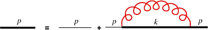
Figure 1: The quark Dyson-Schwinger equation. The curly line represents the strong interaction, the thin line the unperturbed quark propagator, and the solid line represents the dressed quark propagator.

Since for every internal loop there is a factor of $\alpha^{2}=g^{2}/N_{c}$, and a multiplicative factor of $N_{c}$, the color dependence disappears. The vertex corrections and the quark-gluon vertices do not have a multiplicative factor, being supressed in the large $N_{c}$ limit. Therefore, in this limit the rainbow approximation (undressed vertices and the absence of the quark loops from the gluon propagator) is justified thooft .

In Eq. (16) $d^{2}k=dk_{-}dk_{+}$, and since $D(k)$ does not depend on $k_{+}$, the principal part ${\cal P}\int d^{2}k$ does not depend on $p_{+}$. This allows the following parametrization of the full quark propagator,

$$S(p)=\frac{p_{-}\gamma_{+}+\left(p_{+}-\frac{\Sigma(p_{-})}{2}\right)\gamma_{-}+m_{0}}{2p_{-}\left(p_{+}-\frac{\Sigma(p_{-})}{2}\right)-m_{0}^{2}+i\epsilon}\,,$$ (17)

where the self-energy contribution $\Sigma$, originated by ${\cal P}\int d^{2}k$, depends only on $k_{-}$:

$$\Sigma(p_{-})=-\frac{4g^{2}}{(2\pi)^{2}i}{\cal P}\int dk_{-}dk_{+}D(k_{-}-p_{-})\frac{k_{-}}{2k_{-}k_{+}-k_{-}\Sigma(k_{-})-m_{0}^{2}+i\epsilon}\,.$$ (18)

Performing the $k_{+}$ integral first one obtains

$$\int dk_{+}\frac{k_{-}}{2k_{-}k_{+}-k_{-}\Sigma(k_{-})-m_{0}^{2}+i\epsilon}=-\frac{i\pi}{2}\mathrm{sgn}(k_{-})\,.$$ (19)

Substituting this result back into Eq. (18) one finds that

$$\Sigma(p_{-})=\frac{g^{2}}{2\pi p_{-}}{\cal P}\int dk_{-}D(k_{-}-p_{-})\mathrm{sgn}(p_{-})\,.$$ (20)

Using Eq. (13) for $D(k_{-}-p_{-})$ and performing the integral we get

$$\Sigma(p_{-})=-\frac{g^{2}}{\pi p_{-}}\,.$$ (21)

This, in combination with Eq. (17) results in

$$S(p)=\frac{(p_{+}+\frac{g^{2}}{2p_{-}\pi})\gamma_{-}+p_{-}\gamma_{+}+m_{0}}{2p_{+}p_{-}-(m_{0}^{2}-\frac{g^{2}}{\pi}-i\epsilon)}\,.$$ (22)

Note that the masspole has been shifted:

$$m_{0}^{2}\rightarrow m^{2}=m_{0}^{2}-\frac{g^{2}}{\pi}.$$ (23)

Having obtained the dressed propagator, we are ready to proceed to the next stage, namely the calculation of the $q$-$\bar{q}$ bound state.

II.3 Two-body bound states

In the following, we label the dressed quark mass by $m_{1}$. As for the antiquark (which might have a different flavor), we label its dressed mass by $m_{2}$. The total momentum of the bound state is denoted by $r$ and the momentum of the quark by $p$. The momentum of the antiquark is then $r-p$.

The bound state wave function $\Gamma(p,r)$ is given by the Bethe-Salpeter equation (also shown graphically in Fig. 2),

$$\Gamma(p,r)=ig^{2}{\cal P}\int\frac{d^{2}k}{(2\pi)^{2}}D(k_{-})\gamma_{-}S_{2}(p+k-r)\Gamma(p+k,r)S_{1}(p+k)\gamma_{-}\,,$$ (24)

where $S_{1}$ and $S_{2}$ are the quark- and the antiquark propagators, respectively.

Figure 2: The Bethe-Salpeter equation for the $q\bar{q}$ bound state.

With the substitution $\Gamma(p,r)=\gamma_{-}\psi(p,r)$ thooft Eq. (24) becomes

$$\psi(p,r)=i(2g)^{2}{\cal P}\int\frac{d^{2}k}{(2\pi)^{2}}\frac{D(k_{-})(p+k)_{-}(p+k-r)_{-}\psi(p+k,r)}{\left[(p+k)^{2}-m_{1}^{2}\right]\left[(p+k-r)^{2}-m_{2}^{2}\right]}\,.$$ (25)

The equal $x_{-}$ wave function is defined in the following fashion:

$$\varphi(p_{-},r_{-})=\int_{-\infty}^{\infty}dp_{+}\frac{p_{-}(p-r)_{-}\psi(p,r)}{(p^{2}-m_{1}^{2})\left[(p-r)^{2}-m_{2}^{2}\right]}\,.$$ (26)

By substituting this into Eq. (25) one gets

$$\psi(p,r)=\frac{g^{2}}{-i\pi^{2}}{\cal P}\int dk_{-}D(k_{-})\varphi(p_{-}+k_{-},r_{-})\,.$$ (27)

Note that $\psi(p,r)$ does not depend on $p_{+}$. Multiplying both sides of the former equation by $[p_{-}(p-r)_{-}]/[(p^{2}-m_{1}^{2})((p-r)^{2}-m_{2}^{2})]$ and integrating over $p_{+}$ we consider the two poles in the complex $p_{+}$-plane, namely $k_{1}=\frac{m_{1}^{2}}{2p_{-}}-i\epsilon\mathrm{sgn}(p_{-})$ and $k_{2}=\frac{m_{2}^{2}}{2(p_{-}-r_{-})}-i\epsilon\mathrm{sgn}(p_{-}-r_{-})$. If both of them are in the same half plane the integral over $p_{+}$ is zero, because the sum of the two residues is zero. If the first pole is in the upper half-plane and the second one is in the lower half-plane (which means that $p_{-}<0$ and $p_{-}-r_{-}>0$) the integral is $2\pi i/(k_{1}-k_{2})=2\pi i\theta(-p_{-})\theta(p_{-}-r_{-})/(k_{1}-k_{2})$. If the second pole is in the upper half-plane and the first one is in the lower half plane the integral is $-2\pi i\theta(p_{-})\theta(-p_{-}+r_{-})/(k_{1}-k_{2})$. Combining these two cases one obtains

$$\varphi(p,r)=\frac{\pi i}{2}\frac{\theta(-p_{-})\theta(p_{-}-r_{-})-\theta(p_{-})\theta(r_{-}-p_{-})}{\frac{m_{1}^{2}}{2p_{-}}-\frac{m_{2}^{2}}{2(p_{-}-r_{-})}-r_{+}}\psi(p,r)\,.$$ (28)

Whenever the combination of the $\theta$ functions does not vanish, it is easy to invert this relation:

$$\psi(p,r)=\frac{2}{\pi i}\left(\theta(-p_{-})\theta(p_{-}-r_{-})-\theta(p_{-})\theta(r_{-}-p_{-})\right)\left(\frac{m_{1}^{2}}{2p_{-}}-\frac{m_{2}^{2}}{2(p_{-}-r_{-})}-r_{+}\right)\varphi(p,r)\,.$$ (29)

Whenever this condition does not stand, we have to use Eq. (27) to compute $\psi$ from $\varphi$. Note that $\varphi$ has been normalized to $1/\sqrt{N_{c}}$ in order to get the correct charge normalization.

In order to determine $\varphi$, we transform Eq. (26) into a form suitable for a numerical calculation. The $\theta$ functions limit the range of $p_{-}$ to $0<p_{-}<r_{-}$, and for real particles only positive values for $r_{+}$ must be considered. After some algebraic manipulations, Eq. (28) becomes

$$\mu^{2}\varphi(x,r)=\left(\frac{\alpha_{1}}{x}+\frac{\alpha_{2}}{1-x}\right)\varphi(x,r)-{\cal P}\int_{0}^{1}dy\frac{\varphi(y,r)-\varphi(x,r)}{(y-x)^{2}}\,,$$ (30)

where the following notation was introduced:

$$\mu^{2}=\frac{2\pi r_{+}r_{-}}{g^{2}}\,,\qquad\alpha_{1}=\frac{\pi m_{1}^{2}}{g^{2}}\,,\qquad\alpha_{2}=\frac{\pi m_{2}^{2}}{g^{2}}\,,\qquad x=\frac{p_{-}}{r_{-}}\,,\qquad y=\frac{k_{-}}{r_{-}}\,.$$ (31)

We solve the integral equation (30) numerically. The wave function is expanded in cubic splines (since the wave function $\varphi$ is defined only in the range between $x=0$ and $x=1$, the boundary condition that they vanish at the limits of this interval is imposed). The resulting linear matrix equation for the expansion coefficients was solved with standard eigenvalue routines.

In the limit $m_{01}=m_{02}=0$, Eq. (30) yields a ground state of zero mass, and thus is consistent with chiral symmetry. To generate a solution that is related to the pion in the real world, we searched for a bound state solution of Eq. (30) with a mass of $140$ MeV. To obtain such a solution, we varied the bare mass $m_{01}$ of one of the quarks. For simplicity, the second quark mass $m_{02}$ was not taken as an independent free model parameter but determined by assuming a fixed mass ratio $\frac{m_{01}}{m_{02}}=3/4$, which lies within the accepted range between $0.2$ and $0.8$ PDG . The coupling parameter $g$ and the dressed masses $m_{1}$ and $m_{2}$ were adjusted accordingly, through Eqs.(30), (31) and (23).

We represent in Fig. 3 the values of the bare quark mass $m_{01}$, as a function of the coupling strength $g$, which generate a bound state with a mass of $140$ MeV.

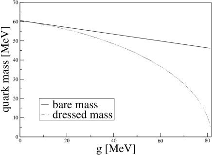
Figure 3: The bare mass (solid line) and the dressed mass (dashed line) of the first quark, as a function of the strong coupling constant $g$, with the constraints that the pion mass is $140$ MeV and the ratio $m_{01}/m_{02}=3/4$.

The bare masses are found to depend linearly on $g$. The slope and the $y$-axis intercept of the numerical straight line on Fig. 3 are easily determined through a fit, with the result

$$m_{01}=60.57-0.178\,g\quad{\rm MeV}\,.$$ (32)

With the help of Eq. (23) we can also predict the dependence of the dressed masses on $g$ from the curves for the bare masses. Therefore, in the ’t Hooft model the dressed masses are given as the following functions of $g$:

$$m_{1}^{2} = (60.57-0.178\phantom{q}g)^{2}-\frac{g^{2}}{\pi}\phantom{q}{\rm MeV}^{2}\,$$

$$m_{2}^{2} = (80.76-0.24\phantom{q}g)^{2}-\frac{g^{2}}{\pi}\phantom{q}{\rm MeV}^{2}\,.$$ (33)

We can also determine the largest value of $g$, such that each dressed mass is physical, i.e., not imaginary. For the first flavor this happens at $g=81.64$ MeV, while for the second flavor at $g=100.8$ MeV. The first value is therefore the largest possible for $g$, such the ’t Hooft model may support a constituent quark model interpretation, where the dressed masses correspond to constituent quark masses.

III Meson-meson scattering

In this section we consider the meson-meson elastic scattering amplitude. We continue to assume two different flavors for the quarks, whose dressed masses are $m_{1}$ and $m_{2}$, and we consider the lowest $q\bar{q}$ bound state only.

The diagrams that dominate in the large $N_{c}$ limit are the quark exchange box diagram, represented in Fig. 4, and the quark exchange crossbox diagram, represented in Fig. 5. In the center of mass system, the momenta of the ingoing mesons are $P=(P^{0},P^{1})=(\sqrt{\mu^{2}+p^{2}},p)$ and ${\tilde{P}}=({\tilde{P}}^{0},{\tilde{P}}^{1})=(\sqrt{\mu^{2}+p^{2}},-p)$, where $\mu$ is the mass of the meson and $p$ the relative momentum. The outgoing particles then have the same (but interchanged) momenta.

Figure 4: The quark-exchange box diagram. The vertex functions are represented by filled circles, and the mesons by double lines. The power counting from the vertices is explicitely shown. An extra factor of $N_{c}$ comes from the color summation in the internal loop.

Figure 5: The quark-exchange crossed box diagram. As in Fig. 4, the power counting factors are explicitely shown. An extra factor $N_{c}$ comes from the color summation in the internal loop.

Both diagrams are symmetrized in terms of the outgoing states. Similar diagrams which are obtained from the former ones by interchanging $m_{1}$ and $m_{2}$ in the intermediate state are also considered. There are a total of eight diagrams which were calculated. When there is only one quark flavor, one does not need to interchange the two masses and there are only four diagrams. The sum of these diagrams is proportional to $1/N_{c}$.

As for the gluon exchange diagrams, such as in Fig. 6, they are suppressed in the large $N_{c}$ limit by a factor of $1/N_{c}$ compared to the quark exchange terms.

Figure 6: The gluon exchange diagram. Power counting is shown as previously. For this purpose the gluon line is represented as two parallel quark lines. An extra factor $N_{c}$ comes from the color summation in the internal loop.

Since the vertex function is independent of the $+$ component of the relative momentum, the momentum integral in the loops of Figs. 4 and 5 is simplified: we can first integrate the propagator products over $k_{+}$ analytically, and then perform numerically the second integration over $k_{-}$, which includes now the vertex functions.

As an illustrative example, we demonstrate the calculation of the box diagram (Fig. 4) in greater detail.

The corresponding scattering amplitude is

$${\cal M}_{\mathrm{box}} = \int_{\infty}^{\infty}dk_{-}\int_{\infty}^{\infty}dk_{+}\psi(-k,-P)\psi(k,{\tilde{P}})\psi(P+{\tilde{P}}-k,P)\psi(k-P-{\tilde{P}},-{\tilde{P}})$$ (34)

$$\times \frac{1}{k_{+}-\frac{m_{1}^{2}}{2k_{-}}+i\epsilon\,\mathrm{sgn}(k_{-})}\frac{1}{k_{+}-{\tilde{P}}_{-}-\frac{m_{2}^{2}}{2(k_{-}-{\tilde{P}}_{-})}+i\epsilon\,\mathrm{sgn}(k_{-}-{\tilde{P}}_{-})}$$

$$\times \frac{1}{k_{+}-P_{+}-{\tilde{P}}_{+}-\frac{m_{1}^{2}}{2(k_{-}-P_{-}-{\tilde{P}}_{-})}+i\epsilon\,\mathrm{sgn}(k_{-}-P_{-}-{\tilde{P}}_{-})}$$

$$\times \frac{1}{k_{+}-P_{+}-\frac{m_{2}^{2}}{2(k_{-}-P_{-})}+i\epsilon\,\mathrm{sgn}(k_{-}-P_{-})}\,.$$

The propagators have four poles:

$$k_{1} = \frac{m_{1}^{2}}{2k_{-}}-i\epsilon\,\mathrm{sgn}(k_{-})\,,$$

$$k_{2} = {\tilde{P}}_{+}+\frac{m_{2}^{2}}{2(k_{-}-{\tilde{P}}_{-})}-i\epsilon\,\mathrm{sgn}(k_{-}-{\tilde{P}}_{-})\,,$$

$$k_{3} = P_{+}+{\tilde{P}}_{+}+\frac{m_{1}^{2}}{2(k_{-}-P_{-}-{\tilde{P}}_{-})}-i\epsilon\,\mathrm{sgn}(k_{-}-P_{-}-{\tilde{P}}_{-})\,,$$

$$k_{4} = P_{+}+\frac{m_{2}^{2}}{2(k_{-}-P_{-})}-i\epsilon\,\mathrm{sgn}(k_{-}-P_{-})\,.$$ (35)

In order to perform the $k_{+}$ integration, one needs to close the contour in the complex plane and consider the residues of all poles inside the contour. There are $16$ different possible combinations of signs of the imaginary parts of the poles. Some of these cases can be excluded, because they correspond to values of $k_{-}$ which make the $k_{+}$ integral vanish.

For instance, a pole $k_{1}$ in the upper half plane implies that the pole $k_{2}$ cannot be in the lower half-plane, otherwise one would have $k_{-}>\tilde{P}_{-}=(\sqrt{\mu^{2}+p^{2}}+p)/\sqrt{2}>0$, in contradiction with the initial hypothesis $k_{-}<0$. Likewise the poles $k_{3}$ and $k_{4}$ cannot be in the lower half-plane either. Therefore, if $k_{1}$ is in the upper half-plane, the other 3 poles are also in the upper half plane. This would imply the $k_{+}$ integral to vanish, since one may close the contour below the $k_{+}$ axis. Therefore we can exclude the case when $k_{1}$ is in the upper half plane.

After a detailed analysis one finds that there are only three cases that have a non-vanishing contribution to the integral: (i) only $k_{3}$ is in the upper half plane, (ii) the poles $k_{2}$ and $k_{3}$ are in the upper half plane, (iii) only $k_{1}$ is in the lower half plane. As for case (i), it implies $k_{-}>{\tilde{P}}_{-}$ and $k_{-}<P_{-}+{\tilde{P}}_{-}$. Under these circumstances, $\psi(P+{\tilde{P}}-k,P)=\frac{2}{\pi i}(k_{3}-k_{2})|_{\epsilon=0}\varphi((P+{\tilde{P}}-k)_{-}/P_{-})$ and $\psi(k-P-{\tilde{P}},-{\tilde{P}})=\frac{2}{\pi i}(k_{2}-k_{1})|_{\epsilon=0}\varphi((P+{\tilde{P}}-k)_{-}/{{\tilde{P}}_{-}})$, due to Eq.  (29), while the other vertex functions have to be evaluated using Eq. (27). The contribution from case (i) becomes

$${\cal M}_{\mathrm{box}}|_{1} = -2\pi i\left(\frac{2}{\pi}\right)^{2}\int_{{\tilde{P}}_{-}}^{{\tilde{P}}_{-}+P_{-}}dk_{-}\frac{1}{(k_{3}-k_{4})|_{\epsilon=0}}$$

$$\times \varphi(\frac{(P+{\tilde{P}}-k)_{-}}{{P_{-}}})\varphi(\frac{(P+{\tilde{P}}-k)_{-}}{{\tilde{P}}_{-}})\psi(-k,-P)\psi(k,{\tilde{P}})\,.$$ (36)

This integral is computed numerically. We treat the other two cases in a similar fashion.

We note that the amplitude of Eq. (36) vanishes in the chiral limit, which supports that the ground state solution for the $q{\bar{q}}$ system has features of the pion. Indeed, since in the chiral limit Eq. (30) gives $\mu=0$, one has $P_{-}=\frac{1}{\sqrt{2}}(\sqrt{\mu^{2}+p^{2}}-p)=0$, implying that the two integration limits in (36) coincide, and therefore the amplitude vanishes. The same can be shown for the other terms of the amplitude not explicitly written here.

It is worth mentioning that we implemented stability tests of the numerical results against the number of gridpoints, the number of splines and the singularity regulator $\epsilon$ (the $k_{+}$ integral of the propagators is singular). These checks proceeded by imposing the following criteria: doubling each of the mentioned parameters, the relative change in the results should be less than 1% . Convergence is typically obtained for 440 gridpoints, 40 splines and $\epsilon=10^{-2}$.

IV Results

The numerical calculation of the meson-meson scattering amplitude (section III) starts with the evaluation of the two-body quark-antiquark wavefunction from the Bethe-Salpeter equation (section II.3). In turn, this demands as input the bare quark masses and the quark-gluon coupling constant $g$ (section II.2).

We constructed four representative models which correspond to four different choices of the quark-gluon coupling constant and bare quark masses. They are subjected to the constraint that the bound state mass of the $q\bar{q}$ system is the pion mass $m_{\pi}$=140 MeV.

	Model I	Model II	Model III	Model IV
$g$	1	20.1	80	2500
$m_{01}$	60.0	57.0	46.4	6.0
$m_{02}$	80.0	76.1	61.8	5.0
$m_{1}$	60.0	55.9	10.6	-
$m_{2}$	80.0	75.2	42.2	-
$m_{r}$ ($=E_{R}$)	280.0	282.4	280.7	300.0
$m_{i}$	4.4	68.6	80.7	139.3
$\Gamma$	0.07	16.4	23.2	64.7

Table 1: Constants and resonance parameters for models I–IV. The first five lines show the quark-gluon coupling constant, the bare the dressed quark masses (the latter are unphysical in model IV and thus not included). The following lines are the results of the s-channel resonance fit using Eq. (37). All parameters are in MeV.

The parameters defining the four models are shown in Table 1. The organization principle for these models is that, going from model I to model IV, the quark-gluon coupling constant increases and the quark masses decrease.

In models I and II, the sum of the dressed quark masses is close to the real pion mass. Consequently, they can be interpreted as constituent quark masses in a constituent quark model for the “pion”, generated by QCD within the ’t Hooft model assumptions. However, this correspondence breaks down for large couplings, as seen for the model considered next.

In model III, the value of the coupling $g$ is chosen slightly below the maximum value determined in section 2 for a constituent quark model interpretation, while in model IV that maximum value is exceeded substantially. In this last case, the dressed masses are imaginary and thus not physical.

Not surprisingly, the bare quark masses differ from the up and down current quark masses of QCD for all models. This is a known artifact of the ’t Hooft model: from Eq. (23) one can see that the mass shift due to the dressing decreases the quark mass, instead of increasing it as in 3+1 dimensional QCD.

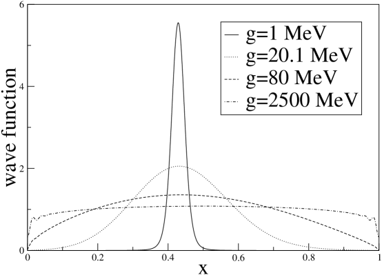
Figure 7: Bethe-Salpeter $q\bar{q}$ wave functions for models I–IV. $x=\frac{p_{-}}{r_{-}}$ is the momentum fraction (or Bjorken variable) defined in Eq. (31).

Figure 7 shows the obtained Bethe-Salpeter $q\bar{q}$ wave functions for each model. Clearly, the description of the quark-gluon vertices varies considerably. The wave functions are strongly peaked around $x$ close to 0.4 for small values of $g$, while for larger $g$ they become broader and more and more constant. This behavior can be easily understood: larger values of $g$ cause stronger attraction between quark and antiquark, leading to a tighter bound state and therefore a more spread out wave function in momentum space.

As described in the previous section, for each of these models we calculated the meson-meson scattering amplitude, the squares of which are displayed in Fig. 8. Since we are primarily interested in their structure, the amplitudes have been scaled such that the maximum of their absolute squares are equal to 1. In all four cases, we find a resonance structure close to threshold.

This feature could be a sign for the existence of a $q^{2}\bar{q}^{2}$ bound state, for which the lattice calculations of Ref. Jaffe found indications. We remind the reader that working in perturbation theory we cannot generate a bound state directly, but it would be interesting to see if in a non-perturbative extension of our calculation, such a bound state would also emerge from the ’t Hooft model.

On the other hand, the experimentally observed resonances have energies well above threshold. It may be necessary to include gluon exchange (not considered in our calculation) and higher order quark exchange terms in the expansion in powers of $1/N_{c}$ in order to achieve a description resembling more closely the real world.

$\begin{array}[]{c@{\hspace{1cm}}c}\psfig{width=202.35622pt}\hfil\hskip 28.45274pt&\psfig{width=202.35622pt}\\ \hfil\hskip 28.45274pt\\ \psfig{width=202.35622pt}\hfil\hskip 28.45274pt&\psfig{width=202.35622pt}\\ \end{array}$

Figure 8: Absolute squares of meson-meson scattering amplitudes for models I – IV close to threshold energies. A resonance structure is clearly visible. The solid lines are obtained using the ’t Hooft model, the dashed lines represent fits to a simple resonance model. The amplitudes are scaled to 1 at their maximum.

In order to determine approximately the position and width of the resonance, we compare the ’t Hooft model amplitudes to a simple resonance model. We calculate the amplitude for an intermediate s-channel resonance at tree level, the absolute square of which is

$$|{\cal M}|^{2}={\tilde{g}}^{4}\frac{1}{(s-m_{r}^{2})^{2}+m_{i}^{4}}\,,$$ (37)

where $m_{r}^{2}$ and $m_{i}^{2}$ are the real part and the imaginary part of the square of the resonance mass, respectively, and ${\tilde{g}}$ is the effective meson-meson-“$\sigma$” coupling constant. We then fit the parameters of this simple model to best reproduce the ’t Hooft model results.

In the non-relativistic limit, (37) becomes

$$|{\cal M}|^{2}\rightarrow{\tilde{g}}^{4}\frac{\frac{1}{4E_{R}^{2}}}{(E-E_{R})^{2}+\frac{m_{i}^{4}}{4E_{R}^{2}}}\,.$$ (38)

We can compare (38) with the well-known Breit-Wigner form,

$$|{\cal M}|^{2}\approx{\bar{g}}^{4}\frac{\Gamma^{2}/4}{(E-E_{R})^{2}+\Gamma^{2}/4}\,,$$ (39)

where $E_{R}$ is the resonance energy, $\Gamma$ is its width, and ${\bar{g}}$ the corresponding coupling strength, and simply read off the relations $\Gamma^{2}=m_{i}^{4}/m_{r}^{2}$ and $E_{R}=m_{r}$.

The parameters obtained in this way for all models are also displayed in Table 1. We verified in an independent fit directly to the Breit-Wigner form (39) that the parameters are not significantly altered in the non-relativistic limit. For comparison, the mass of the “real” sigma resonance is considered to be in the range of 400–1200 MeV, while its width lies in the interval 600–1000 MeV PDG . Clearly, one should not demand too much from the ’t Hooft model with its simplifying assumptions. However, we consider it a significant finding that it predicts a low energy resonance at all, based solely on the leading-order quark exchange diagrams.

In all four cases, the resonance is located very close to threshold, and it is very narrow. The width increases slowly with increasing quark-gluon coupling strength. On the other hand, the resonance position remains more or less unchanged as long as we restrict ourselves to models with real dressed masses (models I to III). Only for model IV, whose coupling constant is considerably larger, the resonance moves away from threshold to about 300 MeV.

One might have expected the resonance energy to increase smoothly and in a more pronounced manner with the quark-gluon coupling strength $g$. However, one has to keep in mind that the included quark-exchange processes do not directly depend on $g$, but only indirectly through changes of the vertex functions and of the dressed quark masses that appear in the quark propagators. Owing to the already mentioned peculiar feature of the ’t Hooft model that dressed quark masses decrease with increasing coupling strength $g$, the latter tend to decrease the resonance energy. Moreover, while a larger $g$ implies an effectively stronger attraction between the two mesons – once they overlap – through the stronger quark-quark attraction, the very probability of this overlap drops in turn, because the spatial size of the mesons decreases. These effects seems to counterbalance each other to a large extent, leaving the resonance position more or less unchanged.

Similarly, that the width of the meson-meson resonance increases with $g$ is also a consequence of the contraction of the mesons caused by the stronger quark-antiquark attraction. This shrinking in size leads to a larger spreading of the meson-$q\bar{q}$ vertex function in momentum space (see Fig. 7), which in turn contributes to the overlap integrals in the included Feynman diagrams in a wider momentum range, thereby broadening the resonance.

Finally, we should mention that our principal finding – the existence of a narrow low-lying resonance in our calculations – does not depend on the particular value chosen as a constraint for the $q\bar{q}$ bound-state mass. If we use, instead of 140 MeV, a much larger or a much smaller value, we find again a narrow resonance close to threshold.

V Conclusions

We calculated various models for quark-antiquark vertex functions within the ’t Hooft model by solving the corresponding $q\bar{q}$ Bethe-Salpeter equation. In all cases, the bare quark masses and the quark-gluon coupling constants were tuned such that the mass of the $q\bar{q}$ bound state coincides with the pion mass.

We found that, within a limited range of coupling constants and bare quark masses, one obtains $q\bar{q}$ bound states with the features of a constituent quark model, i. e., where the meson mass is approximately equal to the sum of the dressed quark masses. On the other hand, for larger values of the quark-gluon coupling constant this constituent quark picture is no longer sustained.

We used the calculated Bethe-Salpeter wave functions to derive meson-meson (“pion-pion”) scattering amplitudes within the ’t Hooft model. They are calculated from the leading-order quark-exchange diagrams. These QCD-based meson-meson amplitudes exhibit a resonance structure close to threshold in all considered cases. We extracted an effective mass and width of this “sigma-like” resonance by comparison with a simple s-channel resonance model where “pions” and “sigmas” instead of quarks are the effective degrees of freedom.

The extracted values are not meant to be completely realistic in the sense that they should reproduce the experimental data, since the ’t Hooft model is QCD only under simplifying assumptions. However, the results of this calculation demonstrate that the ’t Hooft model can accomodate a resonance for the four-quark system, already in the leading-order quark-exchange processes. In those exchange mechanisms, the diquark correlation, given by the quark-antiquark vertex function, plays an important role in determining the energy dependence of the meson-meson scattering amplitude.

The fact that in our ’t Hooft model calculations a narrow resonance lies close to threshold, while the broader sigma resonance is supposed to be located at higher energy, is indicative to the limitations of the ’t Hooft model. It also hints at the importance of higher-order quark exchange processes as well as of gluon exchange contributions (higher order terms in the $1/N_{c}$ expansion), which should be investigated in future work.

VI Acknowledgements

This work was supported by the Fundação para a Ciência e Tecnologia, Portugal, and FEDER, under grant number SFRH/BPD/5661/2001 (Z.B.), CERN/FIS/43709/2001 and POCTI/FNU/40834/2001 (M.T.P and A.S.).

References

- (1) B. D. Serot, J. D. Walecka, Int. J. Mod. Phys. E6, 515 (1997).
- (2) G. Colangelo, J. Gasser, H. Leutwyler, Nucl. Phys. B603, 125 (2001); G. Przeau, Phys. Rev. C 59, 2301 (1999).
- (3) S. Godfrey, N. Isgur, Phys. Rev. D 32, 189 (1985).
- (4) F. E. Close and N. A. Tornqvist, J. Phys. G 28, R249 (2002).
- (5) M. Alford and R. L. Jaffe, hep-lat/0306037.
- (6) G. ’t Hooft, Nucl. Phys. B72, 461 (1974).
- (7) S. R. Cotanch and P. Maris, Phys. Rev. D 66, 116010 (2002).
- (8) F. Gross and J. Milana, Phys. Rev. D 43, 2401 (1991); F. Gross and J. Milana, Phys. Rev. D 45, 969 (1992); F. Gross and J. Milana, Phys. Rev. D 50, 3332 (1994).
- (9) Z. Batiz and F. Gross, Phys. Rev. C 58, 2963 (1998).
- (10) K. Hagiwara it et al., Phys. Rev. D 66, 010001 (2002).