Three-body structure of the low-lying ¹⁷Ne-states

Abstract

The Borromean nucleus ¹⁷Ne (¹⁵O$+p+p$) is investigated by using the hyperspheric adiabatic expansion for a a three-body system. The measured size of ¹⁵O and the low-lying resonances of ¹⁶F (¹⁵O$+p$) are first used as constraints to determine both central and spin-dependent two-body interactions. Then, the ground state structure of ¹⁷Ne is found to be an almost equal mixture of $s^{2}$ and $d^{2}$ proton-¹⁵O relative states, the two lowest excited states have about 80% of $sd$-mixed components, and for the next two excited three-body states the proton-¹⁵O relative $s$-states do not contribute. The spatial extension is as in ordinary nuclei. The widths of the resonances are estimated by the WKB transmission through the adiabatic potentials and found in agreement with the established experimental limits. We compare with experimental information and previous works.

PACS:  21.45.+v, 27.20.+n, 21.10.Dr

1 Introduction

Halo nuclei are weakly bound and spatially extended systems, and they are expected to appear along the driplines, where nucleon single particle $s$ or $p$-states occur with sufficiently small separation energy [1, 2, 3, 4]. Few-body techniques have proved to be very successful to describe them [5]. The core degrees of freedom decouple from the ones of the halo nucleons, and a cluster description of the system becomes then appropriate [6].

Among the halo structures, the three-body Borromean bound systems (where the two-body subsystems are all unbound) are specially challenging [5, 7, 8]. For nuclei the most likely three-body halo candidates are Borromean systems with small binding energy. The reason is that three particles with attractive short-range interactions are more bound than only two of them. This is not necessarily true when also a sufficiently strong repulsive Coulomb interaction or Pauli repulsion is present. Furthermore the core should contain an even number of the nucleons surrounding it, because otherwise one valence nucleon would be pulled into the core leaving at most one with the larger spatial extension of a halo.

Along the neutron dripline the most studied three-body Borromean halos are ⁶He and ¹¹Li. Heavier neutron dripline systems present very interesting challenges, but the interaction ingredients are often not well established or the simple three-body structures are not directly applicable. Examples could be ¹⁴Be, ¹⁹B, ²²C, ³¹F and ³⁴Ne. Since the Coulomb interaction works against halo formation, on the proton dripline the appearance of halos is less likely, and the candidates necessarily require a relatively light core. In fact, heavier halos than Ne are not expected [9]. Still the degrees of freedom describing the core and the surrounding protons may decouple to some extent and a few-body treatment might be justified.

The interest in genuine two-proton decays have increased recently especially due to the improved experimental techniques [10, 11, 12]. This fact has motivated different investigations on light proton rich nuclei. An especially interesting case is the lightest Borromean dripline nucleus ¹⁷Ne (¹⁵O+p+p), whose excited resonance states are promising candidates to decay through direct two-proton emission [13, 14]. However, the structure of ¹⁷Ne is very controversial. The available publications predict very different content of the $s$ and $d$-waves [15, 16, 17, 18]. Inconsistencies prevail even in a very recent and detailed three-body calculation of the structure of ¹⁷Ne [19]. Nevertheless these models are used to predict new features of the delicate Thomas-Ehrman shifts between states in ¹⁷Ne and ¹⁷N [20].

These inconsistencies may be related to the fact that ¹⁵O has a non-vanishing spin which is difficult to handle consistently and therefore sometimes simply ignored. Unfortunately the finite core spin is a crucial ingredient in the structure of the excited resonance states, at least if they have to be related to the measured resonances of ¹⁶F nucleus. We therefore decided to investigate ¹⁷Ne with an established method which is well tested on the neutron dripline [21]. This method employs hyperspheric adiabatic expansion which is especially suited to describe large and weakly bound systems like halo nuclei [22]. Furthermore, simultaneous use of the complex scaling transformation converts the method into an efficient tool to compute three-body resonances [23, 24].

The inconsistencies might perhaps be related to simplified treatments of ¹⁷Ne as a three-body system of a core and two protons. However, all the lowest excited states in the ¹⁵O-core occur with positive parities between 5.2 MeV and 9 MeV with one exception of 3/2^- at about 6.2 MeV. The ground, first and second excited states of ¹⁷Ne occur with negative parities at -0.94 MeV, 0.34 MeV and 0.82 MeV from the two-proton threshold. These energies are small compared to even the lowest-lying core-excited states, which furthermore would have to be combined with proton valence states of negative parity only present in the next shell. Thus two suppressing effects must occur simultaneously to contribute to these states in ¹⁷Ne. In fact these arguments also apply to the third and fourth excited state in ¹⁷Ne although now the energies are only a factor of two smaller than the core-excited states.

The 3/2^- state at 6.2 MeV is then the most likely contributor, but its energy is still relatively high. We can not exclude small contributions form this core excitation but it seems unlikely that the ground state is affected, since then the two protons should pay a prize of combining into either one $d$-wave or two $p$-waves. Again this is double suppression and rather unlikely. Still contributions to the excited states of ¹⁷Ne are not as strongly excluded. In any case such a core-excitation cannot be the origin of the inconsistencies.

Insignificant contributions from core-excitations is equivalent to the assumption of a structureless core. The probability distributions of core and valence particles may still be overlapping provided the corresponding degrees of freedom are dynamically decoupled. The restriction to the smaller Hilbert space in a few-body treatment necessitates a matching renormalization of the interaction achieved by phenomenological constraints on the effective potential. The related difficulty of antisymmetry between core and valence nucleons is approximately accounted for by use of phase equivalent potentials [25].

In the present work we investigate in detail the characteristics of the low-lying states in ¹⁷Ne in a three-body model. We arrive at a consistent picture describing simultaneously the two-body properties of the internal subsystems and the global three-body properties. The contributions to the ¹⁷Ne states from the different partial waves are carefully analyzed. We do not encounter any sign of a break between properties of ground and excited states as a signal of substantial contribution of core-excitation from the possible 3/2^- state. The convergence of the model and possible uncertainties from the details of the two-body interactions are also investigated. In this attempt to arrive at a consistent picture we shall confront our calculations with results from previous work and if possible determine the origin of discrepancies. We already in [26] discussed a specific application to the Thomas-Ehrman shifts.

The paper is organized as follows: In section 2 we describe very briefly the method used to compute three-body bound state wave functions and three-body resonances as well as the proton-proton and proton-¹⁵O interactions. With the three-body model and the input properly defined we then in section 3 discuss the structure of the low-lying states of ¹⁷Ne. The accuracy of the results and the relation to previous works are discussed in sections 4 and 5. We close the paper with a summary and conclusions.

2 Basic ingredients

An accurate description of a three-body system requires a suitable method to solve the Faddeev (or Schrödinger) equations and the interactions between the constituent particles. We first very briefly sketch the method and then we give a few details about the most important of the two-body interactions

2.1 The three-body method

We use the hyperspheric adiabatic expansion method as described in details for instance in [7, 21]. The three-body wave function is a sum of three Faddeev components $\psi^{(i)}(\mbox{\boldmath$x$}_{i},\mbox{\boldmath$y$}_{i})$ ($i$=1,2,3), each of them expressed in one of the three possible sets of Jacobi coordinates $\{\mbox{\boldmath$x$}_{i},\mbox{\boldmath$y$}_{i}\}$. Each component is then expanded in terms of a complete set of angular functions $\{\phi_{n}^{(i)}\}$

$$\psi^{(i)}={1\over\rho^{5/2}}\sum_{n}f_{n}(\rho)\phi_{n}^{(i)}(\rho,\Omega_{i});(\Omega_{i}\equiv\{\alpha_{i},\Omega_{x_{i}},\Omega_{y_{i}}\}),$$ (1)

where $\rho=\sqrt{x^{2}+y^{2}}$, $\alpha_{i}=\arctan({x_{i}/y_{i}})$, $\Omega_{x_{i}}$, and $\Omega_{y_{i}}$ are the hyperspheric coordinates. Writing the Faddeev equations in terms of these coordinates, and inserting the expansions (1), the Faddeev equations can be separated into angular and radial parts:

$$\hat{\Lambda}^{2}\phi_{n}^{(i)}+\frac{2m\rho^{2}}{\hbar^{2}}V_{jk}(x_{i})\left(\phi_{n}^{(i)}+\phi_{n}^{(j)}+\phi_{n}^{(k)}\right)=\lambda_{n}(\rho)\phi_{n}^{(i)}$$ (2)

$$\left[-\frac{d^{2}}{d\rho^{2}}+\frac{2m}{\hbar^{2}}(V_{3b}(\rho)-E)+\frac{1}{\rho^{2}}\left(\lambda_{n}(\rho)+\frac{15}{4}\right)\right]f_{n}(\rho)$$

$$+\sum_{n^{\prime}}\left(-2P_{nn^{\prime}}\frac{d}{d\rho}-Q_{nn^{\prime}}\right)f_{n^{\prime}}(\rho)=0$$ (3)

where $V_{jk}$ is the two-body interaction between particles $j$ and $k$, $\hat{\Lambda}^{2}$ is an angular operator [21] and $m$ is the normalization mass. In Eq.(3) $E$ is the three-body energy, $V_{3b}$ is a three-body potential used for fine-tuning and the functions $P_{nn^{\prime}}$ and $Q_{nn^{\prime}}$ are given for instance in [21].

It is important to note that the set of angular functions used in the expansion (1) are precisely the eigenfunctions of the angular part of the Faddeev equations. Their corresponding eigenvalues are denoted by $\lambda_{n}(\rho)$, and enter in the radial equations (3) as an essential ingredient in the diagonal part of the effective radial potentials:

$$V_{\mbox{eff}}(\rho)=\frac{\hbar^{2}}{2m}\frac{\lambda_{n}(\rho)+15/4}{\rho^{2}}+V_{3b}(\rho)$$ (4)

The complex scaling method [27] amounts to rotation of the hyperradius ($\rho\rightarrow\rho e^{i\theta}$), while the hyperangles remain unchanged [24]. As soon as the rotation angle $\theta$ is larger than the argument of any given resonance, then this resonance together with the bound states is obtained as an exponentially decreasing solution to the coupled set of radial equations (3). The problem of matching with the non trivial Coulomb asymptotics is thus avoided, since the resonance corresponds to a solution with “bound state” asymptotics. It was shown in [24] that the complex scaling method allows reliable calculations of resonance energies, also for three-body systems with the long-range Coulomb interaction.

2.2 Two-body potentials

The two-body potentials must describe the properties of the two-body subsystems. However, unreflected reproduction of the low-lying spectra of the two-body systems is not sufficient. The subsequent use in the context of a specific Hilbert space could be crucial. This becomes particularly evident when a number of degrees of freedom are frozen in the three-body computation while simultaneously also necessary to conserve symmetries of the effective Hamiltonian. An appropriate example is the spin-dependence of the assumed form of the effective two-body potentials. A bad choice can lead to catastrophic results for the three-body system [28].

For the proton-proton interaction we use the parametrization given in [26, 29]. Other choices have been tried as well but the three-body results do not change significantly.

For the proton-¹⁵O interaction spin-dependent operators are indispensable to reproduce the properties of the low-lying ¹⁶F resonances. We parametrize by use of operators that conserve the proton total angular momentum $\mbox{\boldmath$j$}_{p}$=$\ell$+$\mbox{\boldmath$s$}_{p}$ and the total two-body angular momentum $j$=$\mbox{\boldmath$j$}_{p}$+$\mbox{\boldmath$s$}_{c}$, where $\ell$ is the relative orbital angular momentum, and $\mbox{\boldmath$s$}_{c}$ and $\mbox{\boldmath$s$}_{p}$ are the core (¹⁵O) and proton spins, respectively. These operators permit a clear energy separation of the usual mean-field spin-orbit partners $\ell_{\ell+1/2}$ and $\ell_{\ell-1/2}$. It is then possible to use a proton-core interaction such that the low-lying states have well defined $\ell_{j_{p}}$ quantum numbers, like the $d_{5/2}$ states in ¹⁶F. This is especially important when one of these states is forbidden by the Pauli principle, like for instance the $p_{3/2}$ waves in ¹⁰Li [28].

In [26] we introduced an $\ell$-dependent proton-core interaction of the form:

$$V^{(\ell)}_{p-core}(r)=$$

$$S_{c}^{(\ell)}f^{(\ell)}_{c}(r)+S_{ss}^{(\ell)}f^{(\ell)}_{ss}(r)\mbox{\boldmath$s$}_{c}\cdot\mbox{\boldmath$j$}_{p}-S_{so}^{(\ell)}\frac{1}{r}\frac{d}{dr}f^{(\ell)}_{so}(r)\mbox{\boldmath$\ell$}\cdot\mbox{\boldmath$s$}_{p}+\frac{Z_{c}e^{2}}{r}{\rm Erf}(r/b_{c})\;,$$

where the shapes of the central ($f^{(\ell)}_{c}$), spin-spin ($f^{(\ell)}_{ss}$) and spin-orbit ($f^{(\ell)}_{so}$) radial potentials are chosen to be Woods-Saxon functions, $1/(1+\exp{((r-b_{\ell})/a)})$, with the same diffuseness $a$ in all terms. The proton number of the core is $Z_{c}$. The error function ${\rm Erf}$ describes the proton-core Coulomb interaction of a gaussian core-charge distribution. The range parameter $b_{c}$=2.16 fm reproduces the experimental rms charge radius in ¹⁵O of 2.65 fm.

In [26] the parameters of the Woods-Saxon radial potentials were adjusted to reproduce the experimental energies of the four lowest states in ¹⁶F, and simultaneously, after switching off the Coulomb interaction, the energies of the corresponding states in the mirror nucleus ¹⁶N. The resulting parameters are given in table 1.

Table 1: Radius ($b_{\ell}$) and strengths of the central ($S_{s}^{(\ell)}$), spin-spin ($S_{ss}^{(\ell)}$), and spin-orbit ($S_{so}^{(\ell)}$) potentials in Eqs.(2.2) and (6), that correspond to the Woods-Saxon (WS) and Gaussian (G) proton-core interactions, respectively. In (2.2) the diffuseness $a$ is 0.65 fm in all the cases.

$\ell$	$b_{\ell}$ (fm)		$S_{c}^{(\ell)}$ (MeV)		$S_{ss}^{(\ell)}$ (MeV)		$S_{so}^{(\ell)}$ (MeV$\cdot$fm2, MeV)
	WS	G	WS	G	WS	G	WS	G
$0$	3.00	2.60	$-53.91$	$-76.56$	0.92	1.34	–	–
$1$	2.70	2.80	$-19.99$	$-21.42$	0.69	1.04	$-25.0$	$-8.2$
$2$	2.85	2.80	$-58.45$	$-75.89$	0.24	0.32	$-25.0$	$-8.2$

In order to investigate the dependence of the results on the two-body interactions we have constructed an additional proton-core potential with gaussian form factors. Assuming that the (possibly $\ell$-dependent) range of the gaussians is the same for central, spin-spin, and spin-orbit terms we can write the two-body interaction as:

$$V^{(\ell)}_{p-core}(r)=e^{-(r/b_{\ell})^{2}}\left(S_{c}^{(\ell)}+S_{ss}^{(\ell)}\mbox{\boldmath$s$}_{c}\cdot\mbox{\boldmath$j$}_{p}+S_{so}^{(\ell)}\mbox{\boldmath$\ell$}\cdot\mbox{\boldmath$s$}_{p}\right).$$ (6)

The $s$ and $d$-wave parameters are adjusted to reproduce the experimental energies of the 0^-, 1^-, 2^-, and 3^- states in ¹⁶N and ¹⁶F, see table 1. The accuracy is rather good and very similar to the Woods-Saxon case [28] as seen in table 2 where both computed and measured energies are given.

The experimental energies of the second 1^-/2^- doublet is used to adjust the value of the $d$-wave spin-orbit parameter. These two states must come from the coupling of a $d_{3/2}$-wave and the 1/2^- state of the core. In the same way, the measured 1⁺/2⁺ doublet, coming from the coupling of a $p_{3/2}$-wave and the 1/2^- state of the core, is used to determine the $p$-wave interaction (also given in table 1). As seen in the lower part of table 2, the computed resonance energies agree reasonably well with measurements, but the widths are very much larger than the experimental values. The reason is simply that the computed resonances appear above the Coulomb and centrifugal barriers. This in turn is the result of the gaussian form of the attractive central potential combined with the necessary range of about $3$ fm. Then the attraction at the surface pushes the barriers outwards and simultaneously reduces their heights.

It is possible to construct other two-body nucleon-core potentials reproducing as well the widths of the high-lying 1^-/2^- and 1⁺/2⁺ doublets. This would require a more complicated form than Eq.(6) and more than the four parameters used for each partial wave. With the present assumptions we reproduce 6 experimental values for $s$-waves and 10 for $d$-waves. We prefer the simplicity of Eq.(6), because components related to the relatively high-lying $d_{3/2}$ state as well as the $p$-waves in general, as we shall see later, never contribute by more than 4% of the total norm of the wave function. Another potential would essentially not change the results as long as symmetry properties and resonance energies are maintained, see the discussion of accuracy in section 4.

Table 2: The two-body ¹⁶N and ¹⁶F spectra obtained with the gaussian potential specified in table 1. For unbound states we give the corresponding energies and widths $(E_{R},\Gamma)$. The experimental error bars are not specified when they are smaller than the last digit. For unbound states the energies are decay energies above threshold.

$J^{\pi}$	16N	Exp.[30]	16F	Exp.[30]
0-	$-2.37$	$-2.371$	(0.53,$2\cdot 10^{-3}$)	(0.535, $0.040\pm 0.020$)
1-	$-2.09$	$-2.094$	(0.70,$\sim 10^{-5}$)	($0.728\pm 0.006$, $<0.040$)
2-	$-2.49$	$-2.491$	(0.95,0.01)	($0.959\pm 0.005$, $0.040\pm 0.030$)
3-	$-2.19$	$-2.193$	(1.21,0.01)	($1.256\pm 0.004$, $<0.015$)
1+	(0.86,1.22)	(0.86,0.02)	(3.71,3.80)	(4.29$\pm$0.01, $<0.040$)
2+	(1.03,1.86)	(1.03,$<$0.01)	(3.89,4.31)	(4.41$\pm$0.01, $<0.020$)
1-	(2.33,0.96)	(2.27$\pm$0.05,0.25$\pm$0.05)	(5.28,2.27)	(5.81$\pm$0.01,—)
2-	(2.44,1.07)	(2.56,0.02$\pm$0.01)	(5.38,2.41)	—

The Woods-Saxon and Gaussian $s$-wave potentials in table 1 have a deeply bound ¹⁶F-state at $-26.2$ MeV and $-30.5$ MeV, respectively. These states correspond to the $s_{1/2}$ proton states occupied in the ¹⁵O core. They are then forbidden by the Pauli principle, and should be excluded from the calculation. This is implemented as in refs.[29, 25] by use of the phase equivalent potential which has exactly the same phase shifts as the initial two-body interaction for all energies, but the Pauli forbidden bound state is removed from the two-body spectrum. We then use the phase equivalent potential of the central part of the $s$-wave potentials in table 1. Thus the $s$-states actively entering the three-body calculations are the second states of the initial potentials.

The lowest $p$ shell is also fully occupied in ¹⁵O. We should then apply the same treatment as for $s$-waves to the $p$-wave proton-core interaction, using a potential with deeply bound states that are afterwards removed by the corresponding phase equivalent potentials. However, since the $p$ waves basically have no effects in the three-body calculation we use for simplicity the shallow $\ell$=1 potential without bound states as given in table 1. This saves a substantial amount of computing time without loss of accuracy in the calculations.

Partial waves with $\ell>2$ are not crucial for the low-lying states. They should contribute on roughly the same level as the positive parity core-excitations corresponding to energy increases from the $p$ to the $sd$-shell, and perhaps less than the negative parity excitation of ¹⁵O increasing the energy only by the $p$-shell spin-orbit splitting. Quantitative estimates can be obtained with potentials systematically extrapolated from the $\ell=0,1,2$ parameters in table 1. This can then be inferred to indicate that core-excitations are insignificant. In any case the use of effective potentials reproducing the pertinent measured quantities has to be consistent with the choice of model space. Then a phenomenologically adjusted two-body model without core-excitations for ¹⁶F is expected to account correctly for most of the energy in the ¹⁷Ne spectrum.

3 Structure of the ¹⁷Ne states

In this section we discuss the results obtained for the ground and excited states of ¹⁷Ne. We start with the results obtained with the Woods-Saxon (WS) proton-core potential in Eq.(2.2).

Together with the two-body potentials we must specify the components included in the calculations. We give them in subsection 3.1. The output are then the effective potentials entering in the radial part of the Faddeev equations, and the energy spectrum obtained when solving the radial part. The potentials are briefly described in subsection 3.2, and in 3.3 the properties of the computed ¹⁷Ne states are analyzed in detail. We close the section by discussing the spatial distribution of the states and provide a novel WKB estimate of the widths of the resonances in subsections 3.4 and 3.5, respectively.

3.1 Components

We first compute the angular eigenvectors and eigenvalues from Eq.(2). This is done by expanding the eigenvectors in the basis $\{{\cal Y}_{\ell_{x}\ell_{y},L}^{K}(\alpha_{i},\Omega_{x_{i}},\Omega_{y_{i}})\otimes\chi_{s_{x}s_{y},S}\}$, where ${\cal Y}_{\ell_{x}\ell_{y},L}^{K}$ are the hyperspheric harmonics and $\chi$ is the spin function [21]. The quantum number $\ell_{x}$ is the relative orbital angular momentum between particles $j$ and $k$, and $s_{x}$ is the coupling of their two spins. $\ell_{y}$ is the relative orbital angular momentum of particle $i$ and the center of mass of the $jk$ two-body system, and $s_{y}$ is the spin of particle $i$. The coupling of $\ell_{x}$ and $\ell_{y}$, and of $s_{x}$ and $s_{y}$, are $L$ and $S$, respectively, which in turn couple to the total angular momentum $J$ of the system. Finally, $K$=$2n$+$\ell_{x}$+$\ell_{y}$, where $n$ is the usual nodal quantum number.

Table 3: Components included for the $1/2^{-}$ state of ¹⁷Ne. The upper part refers to the Jacobi set where $x$ connects the two protons. In the lower part $x$ connects the core and one of the protons. The sixth column indicates the maximum value of the hypermomentum $K$. The last column gives the contribution of the component to the total norm of the wave function. Only those components contributing more than 1% are given. In each Jacobi set these probabilities should then add up to 100%.

$\ell_{x}$	$\ell_{y}$	$L$	$s_{x}$	$S$	$K_{max}$	$W(^{17}\mbox{Ne})$
0	0	0	0	1/2	100	89.0
1	1	1	1	1/2	52	2.4
1	1	1	1	3/2	62	4.7
2	2	0	0	1/2	54	3.8
0	0	0	0	1/2	60	11.4
0	0	0	1	1/2	80	34.0
2	2	0	0	1/2	60	10.4
2	2	0	1	1/2	84	31.2
2	2	1	0	1/2	34	1.9
2	2	1	1	3/2	44	4.9
1	1	0	1	1/2	42	4.1
1	1	0	0	1/2	42	1.4

Table 4: As table 3 for the $3/2^{-}$ state of ¹⁷Ne.

$\ell_{x}$	$\ell_{y}$	$L$	$s_{x}$	$S$	$K_{max}$	$W(^{17}\mbox{Ne})$
1	1	1	1	1/2	62	5.7
1	1	1	1	3/2	42	1.2
1	1	2	1	1/2	42	5.0
1	1	2	1	3/2	42	5.0
2	2	2	0	1/2	64	9.9
0	2	2	0	1/2	100	47.5
2	0	2	0	1/2	82	25.7
2	2	1	0	1/2	54	3.4
2	2	1	1	1/2	54	1.0
2	2	1	1	3/2	34	0.7
2	2	2	0	1/2	54	3.3
2	2	2	1	1/2	84	10.1
0	2	2	0	1/2	42	1.4
0	2	2	1	1/2	100	32.9
0	2	2	1	3/2	54	4.9
2	0	2	0	1/2	94	21.3
2	0	2	1	1/2	74	14.0
2	0	2	1	3/2	44	4.9

Table 5: As table 3 for the $5/2^{-}$ state of ¹⁷Ne.

$\ell_{x}$	$\ell_{y}$	$L$	$s_{x}$	$S$	$K_{max}$	$W(^{17}\mbox{Ne})$
1	1	1	1	3/2	62	6.8
1	1	2	1	1/2	52	4.2
1	1	2	1	3/2	62	7.3
2	2	2	0	1/2	84	9.1
0	2	2	0	1/2	102	47.6
2	0	2	0	1/2	102	25.0
1	1	2	0	1/2	32	1.0
1	1	2	1	1/2	32	2.1
2	2	1	1	3/2	64	5.8
2	2	2	0	1/2	64	3.6
2	2	2	1	1/2	74	10.6
2	0	2	0	1/2	42	3.1
2	0	2	1	1/2	82	29.1
2	0	2	1	3/2	62	7.0
0	2	2	0	1/2	82	16.6
0	2	2	1	1/2	82	14.2
0	2	2	1	3/2	62	6.6

Table 6: As table 3 for the $7/2^{-}$ state of ¹⁷Ne.

$\ell_{x}$	$\ell_{y}$	$L$	$s_{x}$	$S$	$K_{max}$	$W(^{17}\mbox{Ne})$
2	2	4	0	1/2	44	9.8
0	4	4	0	1/2	54	19.4
4	0	4	0	1/2	54	14.6
1	3	3	1	1/2	54	20.2
1	3	3	1	3/2	44	7.0
3	1	3	1	1/2	54	21.5
3	1	3	1	3/2	44	7.5
2	2	3	0	1/2	124	31.5
2	2	3	1	1/2	94	10.6
2	2	3	1	3/2	94	14.9
2	2	4	0	1/2	64	11.1
2	2	4	1	1/2	84	31.4

Table 7: As table 3 for the $9/2^{-}$ state of ¹⁷Ne.

$\ell_{x}$	$\ell_{y}$	$L$	$s_{x}$	$S$	$K_{max}$	$W(^{17}\mbox{Ne})$
2	2	4	0	1/2	44	9.6
0	4	4	0	1/2	64	18.9
4	0	4	0	1/2	64	14.2
3	1	3	1	3/2	84	29.3
1	3	3	1	3/2	84	27.3
2	2	3	1	3/2	104	56.0
2	2	4	0	1/2	64	11.2
2	2	4	1	1/2	84	30.4
2	2	4	1	3/2	64	1.9

The lowest valence space for the two protons in ¹⁷Ne is the $sd$-shell. Therefore the expected dominating components are $\ell_{x}$=0,2, $\ell_{y}$=0,2. By use of these components and the core-spin and parity of 1/2^-, we can construct three-body states with total angular momentum and parity $J^{\pi}$=$1/2^{-}$, $3/2^{-}$, $5/2^{-}$, $7/2^{-}$, and $9/2^{-}$. Nevertheless, it is only after a full calculation that it is possible to determine precisely which components are needed to reach a given accuracy. For the states mentioned above the components are specified in tables 3 to 7.

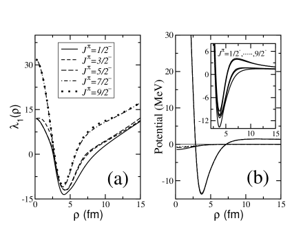
Figure 1: a) The lowest angular eigenvalues $\lambda_{1}(\rho)$ for the $1/2^{-}$, $3/2^{-}$, $5/2^{-}$, $7/2^{-}$ and $9/2^{-}$ states of ¹⁷Ne as function of $\rho$. b) Outer part: Three different effective three-body gaussian potentials that reproduce the experimental two-proton separation energy of the $1/2^{-}$ state in ¹⁷Ne. Their parameters are given in table 8. The curve diverging at the origin is the corresponding effective potentials in Eq.(4). Inner part: Comparison of the deepest effective potential (Eq. (4)) for the different $J^{-}$ states of ¹⁷Ne. The depth of the effective potentials decreases when $J$ increases.

3.2 Effective potentials

In Fig.1a we show the deepest angular eigenvalue $\lambda_{1}$ obtained from equation (2) for each of the $1/2^{-}$, $3/2^{-}$, $5/2^{-}$, $7/2^{-}$, and $9/2^{-}$ states in ¹⁷Ne. Their main characteristics are the hyperspherical values $K(K+4)$ at $\rho$=0, a minimum due to the attractive short-range interaction and a linear increase at asymptotically large distances due to the repulsive Coulomb interaction [31]. The $\lambda$-function starting at 0 ($K$=0) is not present due to the use of the $s$-wave phase equivalent potential removing the deeply bound $s$-state to account for the Pauli principle [25]. Details about the higher $\lambda$-functions are shown in [26].

From the figure we see that the most attractive $\lambda$ function in ¹⁷Ne corresponds to the $1/2^{-}$ state. This agrees with the fact that the $1/2^{-}$ state is the only bound state in ¹⁷Ne with a measured two-proton separation energy of $-944$ keV. Nevertheless, after the computation, the resulting ¹⁷Ne ground state binding energy is $-0.79$ MeV, i.e. 150 keV less bound than the experimental value. This is actually expected, since three-body calculations using pure two-body interactions typically underbind the system. This problem is solved by inclusion of the weak effective three-body potential $V_{3b}$ in Eq.(3), that accounts for three-body polarization effects arising when the three particles all are close to each other. Therefore the three-body potential has to be of short range, and its precise shape is not very relevant, since the overall three-body structure is unchanged. This construction ensures that the two-body resonances remain unaffected within the three-body system after this necessary fine-tuning. The effective total potential entering is then given by Eq.(4).

In the outer part of Fig.1b the curves close to the horizontal zero axis show three gaussian three-body forces with different ranges and strengths adjusted to reproduce the measured two-neutron separation energy of 0.94 MeV for the ground state of ¹⁷Ne. The corresponding effective total potentials given by Eq.(4) are also shown in Fig.1b, but they can not be distinguished from each other within the thickness of the curves. This is because the three-body force is very weak compared to the depth of the full potential and it is furthermore largest for small $\rho$-values, where the total potential is highly repulsive. It is then clear that the main structure of the system can not be significantly modified by the choice of one or another of such three-body interactions. In the inner part of Fig.1b we show the computed effective potentials (4) for the five computed states of ¹⁷Ne. The depth of the potential decreases with increasing total angular momentum. Higher $J$-values correspond then to higher energies of the ¹⁷Ne state.

3.3 Spectrum of ¹⁷Ne

The angular eigenvalues are computed from the effective potentials and used in the radial equations (3). Bound states are obtained as solutions falling off exponentially at large distances. Resonance eigenfunctions are found in complete analogy as exponentially falling solutions to the similar equations obtained after complex rotation of the hyperradius.

Table 8: The 2^nd and 3^rd columns give the experimental and computed bound state ($1/2^{-}$) and decay energies ($3/2^{-}$, $5/2^{-}$, $7/2^{-}$, $9/2^{-}$) in ¹⁷Ne (in MeV). The 4^th to 6^th columns are the strengths of the gaussian three-body forces that for a range of 3.0 fm, 3.5 fm, and 4.0 fm, give rise to computed energies in agreement with the experimental values. The 7^th column is the expectation value of the three-body force with range of 4.0 fm. The last column is the contribution to the norm of the first three terms in the expansion (1) using the three-body potential of range 4.0 fm.

$J^{\pi}$	$E_{exp}$	$E_{comp}$	3.0 fm	3.5 fm	4.0 fm	$\langle V_{3b}\rangle$ (MeV)	$\lambda_{n=1,2,3}$ (%)
$1/2^{-}$	$-0.94$	$-0.79$	$-1.5$	$-0.9$	$-0.6$	$-0.2$	88.5, 11.1, 0.4
$3/2^{-}$	0.34	0.63	$-3.4$	$-2.0$	$-1.4$	$-0.3$	90.7, 8.9, 0.2
$5/2^{-}$	0.82	0.91	$-1.1$	$-0.7$	$-0.4$	$-0.1$	77.2, 16.9, 5.6
$7/2^{-}$	2.05	2.24	$-1.8$	$-1.1$	$-0.8$	$-0.2$	97.5, 2.3, 0.2
$9/2^{-}$	2.60	2.70	$-0.1$	$-0.1$	$-0.1$	$-0.1$	91.9, 4.2, 3.8

Only the $1/2^{-}$ state is bound in ¹⁷Ne with a two-proton separation energy of $-944$ keV. The excitation energies of the four lowest resonance states are [13] 1288$\pm$8 keV, 1764$\pm$12 keV, 2997$\pm$11 keV, and 3548$\pm$20 keV for the $3/2^{-}$, $5/2^{-}$, $7/2^{-}$, and $9/2^{-}$ states, respectively. These excitation energies correspond to the decay energies (energies above threshold) shown in the second column of table 8. The computed states (third column) are all slightly underbound compared to the experiment, but the ordering in the spectrum is correct. Additional small attractive three-body potentials are needed to reproduce the experimental energies. For gaussians we give in table 8 both the necessary strengths for different ranges and the expectation values $\langle V_{3b}(\rho)\rangle$ for the corresponding $J^{\pi}$ solutions. The efficiency of the adiabatic expansion in Eq.(1) is seen in the last column of the table. Already the lowest adiabatic potential accounts for more than 75$\%$ of the probability and in most cases for more than 90$\%$. The contributions from the different three-body potentials can hardly be distinguished.

For the ground state of ¹⁷Ne, we give in the last column of table 3 the percentage of the total norm provided by each of the components defined by the sequence of quantum numbers in the previous columns. These numbers are computed with the three-body potential with range 4 fm, and they do not change significantly when another choice is made. When writing the three-body wave function in the first Jacobi set (upper part of the table) the main contribution of 89% is from $s$-waves, and less than 4% comes from $d$-waves. If we use any of the other two identical Jacobi sets (lower part of the table) the $d$-waves contribute with roughly 50% while 45% is from the $s$-waves and the remaining few percents come from $p$-waves.

It is remarkable that the interference between $s$ and $d$ waves explicitly included in the calculation plays a negligible role and falls below the 1% limit included in the table. The reason is that rotation of the components from one Jacobi set into another preserves the value of the total orbital angular momentum $L$. Then $sd$ terms ($L$=2) in the second and third Jacobi sets must correspond to the almost non contributing {$\ell_{x}$=$\ell_{y}=1$, $L$=2, $S$=3/2} component in the first Jacobi set, since $L$=2 otherwise only arises from $\ell_{x}$=0 or 2 where the antisymmetry dictates zero spin of the two protons. Then $L$=2 and the resulting total spin of $S$=1/2 can not couple to the total angular momentum $1/2$ of the ground state. Thus this type of interferences is essentially excluded.

The unbound excited states of ¹⁷Ne are computed by application of the complex scaling method. The resonances obtained for ¹⁷Ne are extremely narrow with widths much smaller than the accuracy of our calculations. Actually in [14] an experimental lower limit of 26 ps on the lifetime of the two-proton decay of the 3/2^- state is given. This lower limit for the lifetime amounts to an upper limit of $2.5\cdot 10^{-11}$ MeV for the width of the resonance. Thus, application of the complex scaling method allows the use of very small scaling angles. Typically complex scaling angles of $\theta=10^{-5}$ are able to find the ¹⁷Ne resonances. For these scaling angles the complex scaled $\lambda$’s can hardly be distinguished from the non-rotated functions in Fig.1a. The imaginary parts are very small and would appear on the zero line if plotted on the figure.

In tables 4$-$7 we show the largest components included in the calculation of the $3/2^{-}$, $5/2^{-}$, $7/2^{-}$, and $9/2^{-}$ states, respectively. For the $3/2^{-}$ and $5/2^{-}$ states (as for the 1/2^-) the $s$, $p$, and $d$-waves are enough to get an adequate description of the system. Inclusion of $\ell>2$ waves and use of extrapolated potentials does not significantly modify the results. The $s$-wave interaction between proton and core enters only in combinations with the $d$-wave. The component $\{\ell_{x}$=0, $\ell_{y}$=0, $L$=0 } is simply not allowed in the $5/2^{-}$ state (the three intrinsic spins of 1/2 can not couple to 5/2). For the $3/2^{-}$ state rotation of the component $\{\ell_{x}$=$\ell_{y}$=$L$=0, $s_{x}$=1, $S$=$3/2\}$ from the second and third Jacobi sets into the first one contributes very little through the coupling of $\ell_{x}$=1 and $\ell_{y}$=1 due to antisymmetry and angular momentum conservation.

Contrary to the ground state, the $sd$-interferences contribute substantially for both the $3/2^{-}$ and $5/2^{-}$ wave functions. For the $3/2^{-}$ state they give more than 70% of the probability in the first Jacobi set, and about 80% in the other two, see table 4. For the $5/2^{-}$ state these probabilities are roughly 73% in the first Jacobi set and 77% in the second and third, see table 5. In both states the $p$-waves have a significant contribution only in the first Jacobi set, while in the other two sets all the possible {$\ell_{x}$= $\ell_{y}$=1} components give less than 3% of the probability.

For $J^{\pi}$=7/2^- and $9/2^{-}$ (tables 6 and 7) $s$-waves do not contribute if only $s$, $p$, and $d$-waves are included. For $J^{\pi}$=$9/2^{-}$ the $sd$-interferences are not allowed. For the $7/2^{-}$ state in principle the $sd$-interference could contribute only in the second and third Jacobi sets ($L$=2 and $S$=3/2 can couple to 7/2). However, rotation into the first Jacobi set preserves both the $L$=2 and $S$=3/2 values implying $s_{x}$=1 and $l_{x}$=1 due to antisymmetry. These components give a contribution to the norm smaller than 1%. For these two resonance states only proton-core $d$-waves for both $l_{x}$ and $l_{y}$ are significant and appearing in the lower part of tables 6 and 7.

When higher waves are included they do not contribute above the 1% level in the second and third Jacobi sets. The reason is simply that it is too expensive to increase the centrifugal barrier. However, the components in the first Jacobi set follow by rotation. In particular the large components with total orbital angular momentum $L$=3 and $S$=3/2 must correspond to equally large contributions of odd partial waves in the first Jacobi set, which necessarily has $\ell_{x}\geq 3$. For $9/2^{-}$ this is in fact the dominating component. The same happens with the $L$=4 and $S$=1/2 components, that after rotation into the first Jacobi set give important contributions corresponding to $sg$-interferences.

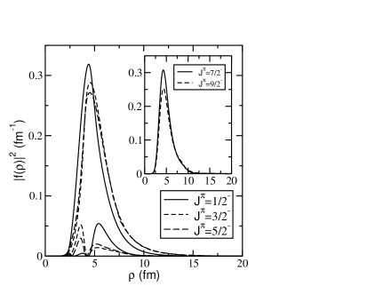
Figure 2: Outer part: Square of the radial wave functions corresponding to the two lowest effective potentials $\lambda_{n}(\rho)$ for the $1/2^{-}$ (solid curves), $3/2^{-}$ (short-dashed curves), and $5/2^{-}$ (long-dashed curves) states of ¹⁷Ne. Inner part: The same as the outer part but for the lowest effective potential $\lambda_{n}(\rho)$ of the $7/2^{-}$ (solid curve) and $9/2^{-}$ (dashed curve) states.

3.4 Spatial distribution

In Fig.2 we show the square of the radial wave functions in the expansion (1). This allows a direct comparison of the contribution of each term to the total wave function. In the outer part of the figure we show the first two terms in the expansion for the states with $J^{\pi}$=1/2^-, 3/2^-, and $5/2^{-}$. For $J^{\pi}$=7/2^- and 9/2^-, shown in the inner part, only the contribution of the dominating term in Eq.(1) is visible.

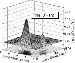
Figure 3: Contour diagram for the probability distribution of the $1/2^{-}$ ground state of ¹⁷Ne. The square of the three-body wave function is integrated over the directions of the two Jacobi coordinates.

The complex scaling method provides bound states and resonances simultaneously as solutions of the complex rotated equation (3) that asymptotically decrease exponentially. The radial solutions in Fig.2 show this asymptotic behaviour already at distances of around 9 fm.

For the excited states of ¹⁷Ne, computed by the complex scaling method, the imaginary parts of the radial functions are very small and only the real parts are visible in the figure. This is a direct consequence of the extremely small widths of these resonances which allow a very small complex scaling angle resulting in almost real wave functions. As for any resonance, the true radial wave function is non-square integrable, diverging at large distances as $\exp{(|\kappa|\rho\sin\beta_{R})}$, where $\beta_{R}$ is the argument of the resonance. Due to the extremely small values of $\beta_{R}$ for the present cases of ¹⁷Ne this divergence has no effect for $\rho$-values up to several hundred fm.

Therefore, up to distances around 40-50 fm we can treat the resonances as bound states, and compute observables like $\langle\rho^{2}\rangle$, $\langle x^{2}\rangle$ or $\langle y^{2}\rangle$, that give information about the spatial distribution of the three-body system. For each state, we give in table 9 such characteristic root mean square distances between the particles. The root mean square radius of the whole three-body system $\langle r^{2}\rangle^{1/2}$ in the $1/2^{-}$ ground state is 2.8 fm consistent with the experimental value of 2.75$\pm$0.07 fm given in [32].

Table 9: For the different computed states of ¹⁷Ne, root mean square distances $\langle r^{2}_{pp}\rangle^{1/2}$, $\langle r^{2}_{c,pp}\rangle^{1/2}$, $\langle r^{2}_{cp}\rangle^{1/2}$, $\langle r^{2}_{p,cp}\rangle^{1/2}$, $\langle\rho^{2}\rangle^{1/2}$, and $\langle r^{2}\rangle^{1/2}$, where $p$ and $c$ denote a halo proton and the core, respectively. All the distances are given in fm. The results do not depend on the three-body interaction chosen from table 8.

$J^{\pi}$	$\langle r^{2}_{pp}\rangle^{1/2}$	$\langle r^{2}_{c,pp}\rangle^{1/2}$	$\langle r^{2}_{cp}\rangle^{1/2}$	$\langle r^{2}_{p,cp}\rangle^{1/2}$	$\langle\rho^{2}\rangle^{1/2}$	$\langle r^{2}\rangle^{1/2}$
$1/2^{-}$	4.5	3.2	3.9	3.9	5.3	2.8
$3/2^{-}$	5.3	3.4	4.3	4.4	5.9	2.9
$5/2^{-}$	5.5	3.5	4.3	4.4	5.9	2.9
$7/2^{-}$	5.6	3.5	4.3	4.5	6.0	3.0
$9/2^{-}$	5.7	3.6	4.4	4.5	6.1	3.0

The structures derived from these mean values are crudely speaking triangles where the distance between the two protons is slightly larger than the distance between proton and core. The dimension increases with angular momentum. A more detailed view is obtained in the contour diagram in Fig.3. We plot the square of the three-body wave function multiplied by the phase space factors and integrated over the directions of the two Jacobi coordinates. We observe that a prominent peak is found for distances between the two protons of about 2 fm and the two-proton center of mass distance to the core of about 3 fm. Another smaller peak is found for corresponding distances of about 5 fm and 1 fm, respectively. These two shapes can be described as two protons either on the same side of the core (at some distance apart) or at almost opposite sides of the core. The structures of the excited states are very similar apart from the dimension increasing with $J$.

The distribution overlaps to some extent the core density with the potential danger of violating the basic few-body assumptions. However, an assessment of model validity is only possible by comparing many predictions with measured observables.

The size of a three-body system is for quantum halos related to the binding energy. The repulsive Coulomb potential may provide a very small binding energy but at the same time confining the structure spatially. The characteristic halo features are revealed by the hyperradial extension measured in units of an appropriate length scale $\rho_{0}$, designed in [8] to measure the content of non-classical probability. In our calculation we have $\rho_{0}\approx 5$ fm, which implies that the dimensionless measure of the binding energy $mB\rho^{2}_{0}/\hbar^{2}$ is around 0.6 and the mean square hyperradius in units of $\rho^{2}_{0}$ is about 1.2. This wave function is therefore to a large extent in the classically allowed region and the properties cannot be obtained by scaling relations independent of the details of the interactions. The ¹⁷Ne system is not a quantum halo as defined in [8] although the structure still can be described as a three-body system.

3.5 Widths of the resonances

The positive energies of the excited states imply that they can decay into three separate particles and also to lower-lying states by electromagnetic transitions. However, the widths of the resonances are very small and beyond the accuracy of the otherwise very efficient complex scaling method. Fortunately the hyperspherical adiabatic method provides generalized radial potentials which are responsible for the three-body bound state structure as well as the asymptotic behavior of the continuum wave functions. The decay widths into separate free particles can then be estimated in the WKB approximation. This is especially tempting since about 90% of the wave function is described by the lowest adiabatic potential and since the widths are small and the effective barrier is smooth. In [31] the accuracy of the WKB approximation was estimated for a system of three charged particles. The WKB turned out to be accurate to within a factor of five including the uncertainty from the preexponential factor, the “knocking rate”.

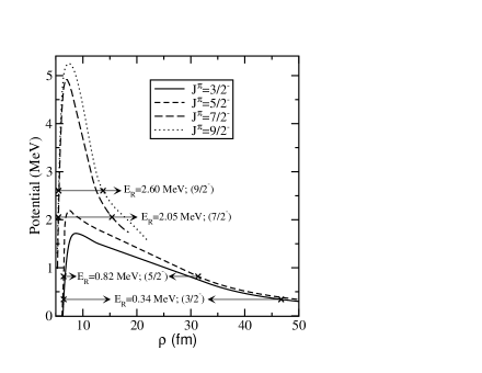
Figure 4: Barrier of the most contributing effective potential for the $J^{\pi}$=$3/2^{-}$, $5/2^{-}$, $7/2^{-}$, and $9/2^{-}$ resonances in ¹⁷Ne. The crosses show the turning points and the arrows show the energies corresponding to each of the resonances.

This use of the WKB approximation, where the lowest adiabatic potential provides the tunneling barrier, is a rather subtle application. There is a striking resemblance with computation of $\alpha$-decay widths from tunneling through centrifugal and Coulomb barriers. However, $\alpha$-decay is assumed to be a two-body process where the $\alpha$-particle is formed with some probability and then tunnels through the two-body barrier. The two-proton decay is a three-body problem and it is only due to the efficiency of the hyperspheric expansion that one suitable generalized potential becomes available. The tunneling probability through the corresponding barrier is, in the one $\lambda$-approximation, then precisely describing the resonance width for decay into the corresponding channel of three particles in the final state. On this level there is a complete equivalence with the $\alpha$-decay computation. The WKB expression is then a rather good approximation to the full three-body coupled channel problem under the two conditions that the lowest adiabatic hyperspheric potential and the WKB-approximation both provide sufficient accuracy.

We therefore have to compute the transmission coefficient through the barrier of the lowest effective potential $V_{\mbox{eff}}$ (see Eq.(4)) constructed by using the dominating angular eigenvalue, see Fig.1b. If crossings of potentials occur along the way through the barrier we follow the path determined by minimum change of the wave function. This corresponds to a path along the most smooth adiabatic potential in full agreement with the basic assumptions of the WKB approximation. Thus the WKB transmission coefficient is estimated by

$$T=\exp{\left\{-2\int_{\rho_{i}}^{\rho_{o}}\left[\frac{2m}{\hbar^{2}}(V_{\mbox{eff}}(\rho)-E_{R})\right]^{1/2}d\rho\right\}}\;,$$ (7)

where $E_{R}$ is the energy of the resonance, and $\rho_{i}$ and $\rho_{o}$ are the inner and outer classical turning points defining the distance through the barrier. In Fig.4 we show the barriers of the resulting effective potential for the four resonances in ¹⁷Ne with $J^{\pi}=3/2^{-},5/2^{-},7/2^{-}$ and $9/2^{-}$. The outer turning points of the effective potentials are located at distances of around 15 fm for the $7/2^{-}$ and $9/2^{-}$ states, above 30 fm for the $5/2^{-}$ resonance, and above 45 fm for the $3/2^{-}$ resonance. These potentials, and therefore the angular eigenvalues, must then be computed accurately below these values. Inaccuracies typically produce too high eigenvalues and therefore too large barriers with too small transmission coefficients or equivalently too small widths.

Table 10: Turning points, frequency, transmission coefficients, average lifetimes, and resonance widths for the $3/2^{-}$, $5/2^{-}$, $7/2^{-}$, and $9/2^{-}$ resonances in ¹⁷Ne. $\rho_{i}$ and $\rho_{o}$ are given in fm, $f$ in MeV/$\hbar$, $t_{a}$ in s, and $\Gamma$ in MeV.

$J^{\pi}$	$\rho_{i}$	$\rho_{o}$	$f$	T	$t_{a}$	$\Gamma$
$3/2^{-}$	6.4	46.7	3.90	$9.2\cdot 10^{-13}$	$1.8\cdot 10^{-10}$	$3.6\cdot 10^{-12}$
$5/2^{-}$	6.4	31.3	3.82	$3.3\cdot 10^{-11}$	$3.6\cdot 10^{-12}$	$1.3\cdot 10^{-10}$
$7/2^{-}$	5.5	15.4	1.54	$3.7\cdot 10^{-3}$	$1.2\cdot 10^{-19}$	$5.6\cdot 10^{-3}$
$9/2^{-}$	5.5	13.7	1.59	$3.3\cdot 10^{-3}$	$1.2\cdot 10^{-19}$	$5.3\cdot 10^{-3}$

Once the transmission coefficient is computed, the decay constant can be obtained as $\Gamma/\hbar$=$fT$, where the frequency $f$ is given in terms of the radial extension $\rho_{i}$ of the attractive pocket and the velocity $v$ of the particle moving in it, i.e. $f$=$v/\rho_{i}$. We estimate the velocity $v$ by equating the kinetic energy ($mv^{2}/2$) and the maximum potential energy $E_{R}$+$|V_{\mbox{eff}}^{(min)}|$, where $|V_{\mbox{eff}}^{(min)}|$ is the maximum depth of the effective potential. This estimate of the knocking rate can easily be off by a factor of two. Furthermore this computation implicitly assumes that the preformation factor is unity, i.e. that the decaying state really is a three-body state consisting of two protons outside the ¹⁵O core.

Finally, the average lifetime $t_{a}$ or the width $\Gamma$ of the resonances are found by inverting the decay constant or multiplying by $\hbar$, respectively. In table 10 we summarize the results for the different resonances. The computed width of the $3/2^{-}$ resonance is consistent with the upper limit of $2.5\cdot 10^{-11}$ MeV quoted in [14]. This limit is in fact essentially theoretical as obtained in a shell model calculation for the magnetic dipole deexcitation probability. The lack of protons in the experiment then leads to the conclusion that the width must exceed the computed electromagnetic value.

Similarly a lower limit for the two-proton decay of the $5/2^{-}$ resonance is deduced to be about $3\cdot 10^{-10}$ MeV [14] which is about three times larger than our crude calculation shown in table 10. The two higher-lying resonances have much larger widths of about 5 keV due to the higher energies and the rather narrow barriers. This behavior can not be predicted from angular momentum and energy systematics. The three-body model is indispensable, not only because the final state asymptotically consists of three particles but more interestingly because the short and intermediate distances determine the widths.

4 Accuracy of model results

The calculated results can not be more reliable than the model. The basic assumptions are that the active few-body degrees of freedom are responsible for all the computed properties. The intrinsic constituent particle degrees of freedom are only implicitly treated through the properties of the two-body interactions. Polarization effects are included but not explicit contributions from intrinsic structure. Therefore cluster models are most suited in descriptions of halo systems while individual applications beyond halos still can be rather accurate if the different degrees of freedom are sufficiently weakly coupled.

Ultimately only practical tests can decide on the issue of model reliability. However, a necessary prerequisite is a series of accuracy tests of the model itself. This means that the numerical methods must reach convergence to the requested level of accuracy. This is not trivial in the present type of cluster computations. Another source of uncertainty is the parametrization of the interactions, e.g. spin-dependence, radial form factors and the numerical values of the parameters. We shall in this section report on these tests.

4.1 Convergence and basis expansion

The convergence of the calculations must be reached at three different levels. First, in the hyperspheric adiabatic expansion of Eq.(1) the number of included potentials must be sufficient. This was shown in the last column of table 8. Typically three terms are enough to provide contributions to the wave functions larger than 99% of the probability. Sometimes one more adiabatic potential has to be included for additional confidence.

Second, the expansion of the angular eigenfunctions $\phi_{n}^{(i)}$ in Eq.(2) in terms of hyperspherical harmonics has to contain all the components giving a relevant contribution to the wave functions. These are the components shown in tables 3 to 7. Together with them, additional components giving contributions smaller than 1% have also been included in the calculations.

Third, once the components have been chosen, convergence must be secured in the expansion in hyperspherical harmonics by requiring inclusion of a sufficiently large number of them, i.e. ${\cal Y}_{\ell_{x}\ell_{y},L}^{K}(\alpha_{i},\Omega_{x_{i}},\Omega_{y_{i}})$. For each component we include all these basis functions with hyperspherical quantum number less than a maximum number $K_{max}$ which may depend on the quantum numbers of the components. We should emphasize that the basis sizes we discuss are for each Faddeev component, i.e. related to each Jacobi coordinate system. If only one Jacobi set is used a much larger $K_{max}$ is necessary for convergence.

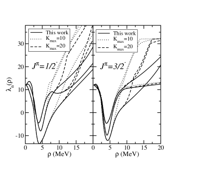
Figure 5: Comparison of the computed $\lambda$ functions for different values of $K_{max}$ for the ¹⁷Ne states $J^{\pi}=1/2^{-}$ (left) and $J^{\pi}=3/2^{-}$ (right). The solid curves are the results with $K_{max}$ from tables 3 and 4.

In the calculations this hypermoment $K_{max}$, given in the sixth column of tables 3-7, is by far large enough to reach convergence in the region of contributing $\rho$-values. This is illustrated in Fig.5 where we show the three first angular eigenvalues, the $\lambda$-functions, for the $1/2^{-}$ and $3/2^{-}$ states in ¹⁷Ne for three different values of $K_{max}$. For the ground state we observe that at a distance of around 7 fm the lowest $\lambda$ with $K_{max}$=10 begin to differ from the converged result. From Fig.2 we see that this significantly can modify the tail of the $1/2^{-}$ radial wave function. In fact, using the three-body interactions given in table 8 the two-neutron separation energy of the $1/2^{-}$ state with $K_{max}$=10 is only $-0.58$ MeV, almost 400 keV less bound than in the full calculation. For $K_{max}$=20 the discrepancy from the converged lowest $\lambda$ for $J^{\pi}$=1/2^- begins at distances larger than 10 fm, and the effect on the radial wave function is not important. When $K_{max}$=20 the two-neutron separation energy is $-0.93$ MeV, pretty close to the one we obtained. Therefore for the ground state at least a value of $K_{max}$=20 is needed.

For the first excited state, $3/2^{-}$, the discrepancies between the different calculations begin at lower distances, see Fig.5. When $K_{max}$=10 the lowest $\lambda$ begins to differ from the other calculation already at $\rho$=6 fm. At this value of $\rho$ the radial wave function in Fig.2 is close to its maximum, and therefore the results obtained with $K_{max}$=10 are not reliable. Actually, the $3/2^{-}$ resonance energy obtained in this case is above 700 keV, more than a factor of two higher than in the full calculation. For $K_{max}$=20 the computed $3/2^{-}$ resonance energy is still 15% higher than the 340 keV obtained in the full calculation. The same kind of convergence is seen for higher values of $J$.

We can then conclude that for the excited states of ¹⁷Ne values of $K_{max}$ higher than 20, typically around 30, are desirable. As shown in tables 4-7 we used in our calculations $K_{max}$ values significantly larger than 30 for some of the components. This is because the estimates of the widths of the resonances require accurate effective potentials for much larger distances than 10 fm, e.g. up to about 50 fm for the $3/2^{-}$ resonance. This accuracy is achieved with the $K_{max}$ values given in the tables. Thus reliable width calculations in a three-body model require a rather large individual basis for each of the Faddeev components related to the different Jacobi sets.

4.2 The shape of the radial potential

In this section we investigate the dependence of the results on the radial shape of the nuclear two-body interactions. The results discussed so far have been obtained with the proton-proton interaction (G) from [26, 29] and the Woods-Saxon (WS) proton-core interaction in Eq.(2.2).

Let us consider now also the gaussian (G) proton-core interaction given in Eq.(6) and table 1 and the sophisticated Argonne (A) proton-proton interaction $v_{18}$ described in [33]. This is a nonrelativistic potential that reproduces $pp$ and $np$ scattering data for energies from 0 to 350 MeV, $nn$ low-energy scattering data, and the deuteron properties. Different combinations of these potentials permit comparison and reliability tests of the results. The calculations are denoted G+WS, A+WS, G+G, …, where the first and second labels refer to the proton-proton and proton-core interactions, respectively.

Figure 6: Comparison between the deepest $\lambda$-functions for the $1/2^{-}$, $3/2^{-}$, and $5/2^{-}$ states in ¹⁷Ne when different proton-proton and proton-core interactions are used (G=Gaussian, WS=Woods-Saxon, A=Argonne). In the label the first symbol refers to the proton-proton potential and the second to the proton-core.

We have repeated all the three-body calculations for the G+G and A+WS cases. The decisive $\lambda$-functions entering in the radial equations (3) are compared in Fig.6 for the $1/2^{-}$, $3/2^{-}$, and $5/2^{-}$ states in ¹⁷Ne. At large distances the $\lambda$-functions are basically identical in the three calculations, since the low energy properties of the two-body potentials are the same. At short distances some differences are visible. The G+G calculations produce a slightly less deep pocket in the potentials than in the other two cases. This means that the phenomenological three-body potentials needed to fit the measured energies of the ¹⁷Ne states are also slightly different.

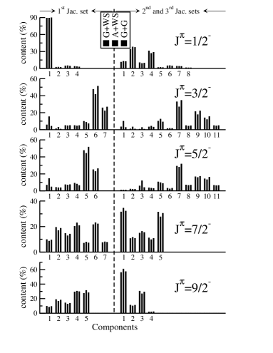
Figure 7: Comparison of the weights of the components for the ¹⁷Ne states. The left part refers to the first Jacobi set and the right to the second and third Jacobi sets. The components are ordered as in tables 3-7. For each component the three bars, from left to right, refer to the G+WS, A+WS, and G+G computations, respectively.

In total, after fitting the resonance energies in ¹⁷Ne by use of gaussian three-body forces, the results are essentially the same as the G+WS results previously discussed. The radial wave functions are hardly distinguishable from the ones shown in Fig.2. In Fig. 7 we compare the weights of the components for the three calculations and the five computed states in ¹⁷Ne. The components are ordered as in tables 3 to 7. The left part of the figure corresponds to the components when the full three-body wave function is written in the first Jacobi set, and the right part to the ones in the second and third Jacobi sets. The three computations give very similar results. For each state the dominant components are the same in all the three cases, and the overall three-body structure is essentially unchanged.

We can then conclude that details like the radial shapes of the two-body interactions are not changing the properties of the three-body system within the accuracy provided by the inherent accuracy of the model.

5 Previous works

Different theoretical works concerning the structure of ¹⁷Ne can be found in the literature. Most of them [15, 17, 18] focus only on the ground state structure and in particular on the weight distribution of the $s$ and $d$-waves. Only [16] and [19] report on more detailed calculations of the ¹⁷Ne spectrum.

In [16] the three-cluster generator coordinate model is used to obtain ¹⁷Ne. The proton-proton interaction is adjusted to reproduce the experimental binding energy. Although no numbers are quoted, the $s$-wave contribution is expected to dominate. The same conclusion is reached in [17] where they analyze the experimental parity dependence of the Coulomb shifts of the $A$=17 isoquartets. They used harmonic oscillator wave functions with a state dependent radius and the Coulomb potential of a uniformly charged sphere. The two protons of the ground state of ¹⁷Ne then seem to occupy the $s_{1/2}$-orbits.

In [18] the $d^{2}$-configuration is for the first time found to dominate in the ground state of ¹⁷Ne. This is concluded by investigating the $\beta^{+}$ decay to the first excited state of ¹⁷F. The decay is found to be roughly a factor of two larger than expected from the nuclear matrix elements that reproduce the $\beta^{-}$ decay into ¹⁷N. In [15] the domination of the $d^{2}$-configuration is confirmed by investigating the difference in Coulomb energy for $s$ and $d$-orbitals. They use Woods-Saxon potentials and an uniformly charged sphere. A coupling of either two $s_{1/2}$ or two $d_{5/2}$-protons to the $A$=15 core immediately reveals that the $d^{2}$-component dominates. To reproduce the measured ¹⁷Ne two-proton separation energy around 78% of the wave function must be of $d^{2}$-character.

Table 11: Computed $s$, $p$, and $d$ wave contents in the ¹⁷N (upper part) and ¹⁷Ne (lower part) wave functions. The results in parenthesis are the ones obtained in ref.[19].

$J^{\pi}$	$s$	$p$	$d$
$1/2^{-}$	38.9 (39.8)	6.7 (4.5)	54.4 (55.6)
$3/2^{-}$	32.8 (36.8)	2.2 (3.0)	65.0 (60.0)
$5/2^{-}$	32.9 (34.5)	4.2 (3.2)	62.9 (61.6)
$1/2^{-}$	45.4 (48.1)	5.6 (4.0)	49.0 (47.8)
$3/2^{-}$	39.2 (38.1)	2.1 (2.8)	58.7 (58.4)
$5/2^{-}$	37.4 (36.2)	3.3 (3.0)	59.3 (60.1)

A detailed calculation of ¹⁷Ne and ¹⁷N has been reported recently in [19]. A three-body model is employed and Woods-Saxon potentials between the three pairs of particles are used. The weight of the different partial waves for the ground state contains around 40% and 48% $s$-wave in the ¹⁷N and ¹⁷Ne wave functions, respectively. These values decrease for the first and second excited states, where the $s^{2}$-wave content varies from case to case between 34.5% and 38.1%. In table 11 we compare our results to the ones given in [19]. For completeness we also include our results for the ¹⁷N case. The agreement is rather good in all the cases. However, apparently in [19] interferences between $s$ and $d$ waves are not considered, while we have found that for the excited states they are crucial. Furthermore, it is not easy to understand how two protons in the $s_{1/2}$-waves can give rise to the excited $5/2^{-}$ state, provided the ¹⁵O core still has spin of 1/2. It is also important to remember that by $\ell$-wave content we refer to the weight of the components in tables 3$-$7 containing that value of $\ell$. In this way, our $\ell_{x}$=$\ell_{y}$=0 components are not fully equivalent to the $s^{2}$-content in the shell model sense.

The spectrum of ¹⁷Ne is previously investigated only in [16] and [19]. In [16] the nucleon-nucleon interaction is adjusted to reproduce the ¹⁷Ne ground state binding energy, but the same interaction is not able to describe the ¹⁶N and ¹⁶F spectra. Even the level order is wrong and the 3^- level comes out as the ground state in both cases. For the three-body systems the ground state angular momentum is correct in [16], but the 3/2^- and 5/2^- levels are reversed compared to the experimental data. The lack of consistency between the two-body interaction needed to reproduce the three-body ground state and the one reproducing the two-body spectra of the two-body subsystems is certainly a weak point in this calculation.

The same deficiency is present in [19], where the three-body structure in ¹⁷Ne obtained with the two-body interactions that reproduce the ¹⁶F spectrum also reverse the positions of the $3/2^{-}$ and $5/2^{-}$-states. The $5/2^{-}$-level is even bound by $-0.41$ MeV, while the $3/2^{-}$-state has an energy above threshold of 0.89 MeV. A three-body force adjusted for each of the states is needed to restore the level order and the positions as found in experiments. It is then clear that the three-body force is forced to play a too important role, since the $5/2^{-}$ energy is moving up from $-0.41$ MeV to the experimental 0.82 MeV and simultaneously the $3/2^{-}$ is moved down in energy.

In the present work these problems are not encountered. When only the two-body forces describing the proton-proton and ¹⁶F properties are used, the energies of the ¹⁷Ne states are the ones in the third column of table 8. They follow the experimental ordering, and use of a small effective three-body force is enough to fit the experimental energies.

The fact that in [19] the same inversion as in [16] appears can be related to the inappropriate spin dependent operators used in the two-body nucleon-core interaction. Contrary to the present work the interaction in [19] is mixing the $d_{3/2}$ and the $d_{5/2}$-states used as an essential part of the valence space for the outer nucleons. The low-lying resonances in ¹⁶N and ¹⁶F do not have the desirable pure $d_{5/2}$-character [28].

Finally the partial two-proton decay widths of the three-body resonances are estimated in the present work, see table 10. In [19] the widths of the $3/2^{-}$ and $5/2^{-}$-states are found to be $4.1\cdot 10^{-19}$ MeV and $1.2\cdot 10^{-11}$ MeV, respectively smaller by seven and one order of magnitude compared to our results. This computed $3/2^{-}$ value is in apparent agreement with the experimental limit. However, their computed width of the $5/2^{-}$ resonance is already at least one order of magnitude too small. The eight orders of magnitude difference between these two computed values seem to be in clear disagreement with measurements which indicates that the lowest and highest of these resonances have widths slightly below and above the electromagnetic decay widths.

The origin of these discrepancies can not be decided without full repetition of all computations. Two effects are perhaps important in this connection. The first is that the basis size has to be rather large to provide a sufficiently accurate description all the way up to the relatively large distances where important contributions to the widths are determined. Too small a basis would usually lead to too high potential energies and therefore too large barriers and too small widths. The maximum hypermoment must be very large when only hyperharmonics in one Jacobi set are used.

The second effect is that the hypersherical adiabatic expansion in principle includes all decay channels, i.e. also sequential decay which often is the dominating mode. For the $3/2^{-}$-state this is apparently not allowed due to energy conservation. However, a kind of virtual decay, where the tail of the two-body resonance is exploited, would enhance the decay probability. This effect is included in our formulation since the two-body resonance configuration influences the lower adiabatic potentials to fairly large hyperradii. This effect is difficult to catch with the direct hyperharmonic expansion method.

6 Summary and conclusions

The structure of the lightest Borromean nucleus ¹⁷Ne is investigated in details in a three-body model where two protons surround the ¹⁵O core. We use the hyperspheric adiabatic expansion method with two-body interactions adjusted to reproduce the properties of the two-body subsystems. The spin-dependent form of the proton-core interaction must be consistent with the mean-field approximation. Otherwise the assumed decoupling of core and valence motion is violated due to the Pauli principle and the angular momentum conservation. We use two different radial shapes for the proton-core potential both consistent with the measured size of ¹⁵O. The Coulomb potential is derived from a gaussian charge distribution with the measured root mean square radius.

The three-body ground state and four measured excited states of ¹⁷Ne are computed. The structure for the ground state is found to be about 45% of $s^{2}$ ($\ell_{x}$=$\ell_{y}$=0) and 50% of $d^{2}$ ($\ell_{x}$=$\ell_{y}$=2) proton-core components. For the two lowest excited states the $sd$ relative proton-core states are dominating while only roughly 18% is of $d^{2}$-character. For the two highest resonances, $d^{2}$-components dominate completely in the second and third Jacobi sets, while contributions from higher partial waves ($sg$ and $pf$-components) can be important in the first Jacobi set. Properties of these states are not computed in previous works.

The spatial distribution is slightly more extended than for ordinary nuclei and with a clear tendency to show two components, i.e. one where the protons and the core are distributed in a triangle and one where the protons try to be on opposite sides of the core. The distribution is not in the classically forbidden region and the scaling relations specific for quantum halos are not obeyed. The criteria for quantum halos are not fulfilled. Still the three-body model seems to give a rather good description of the structure of these five lowest-lying states. The two-proton decay widths are computed by use of the WKB approximation applied on the adiabatic potentials. The computed results are within the experimentally determined limits. The width estimates employ a recently established but non-trivial formulation which relies on the efficiency of both the hyperspheric adiabatic method and the separation at small and intermediate distances of the intrinsic and the necessary asymptotic three-body degrees of freedom.

Accuracy of these computations can be divided into three parts, i.e. (i) model assumptions related to its applicability, (ii) input determination, uniqueness and reliability, (iii) numerical accuracy including convergence of expansions. First the consistency of the results supports the credibility of the model. Second we carefully evaluated the accuracy both by testing for convergence and by using different two-body interactions.

In conclusion, the three-body model describes efficiently the cluster structure of ¹⁷Ne. The hyperspheric adiabatic expansion in the same framework provides consistently also the simple semiclassical estimates of resonance decays into three-body final states.

7 acknowledgments

We want to thank Hans Fynbo for useful suggestions and discussions.

References

- [1] P.G. Hansen, A.S. Jensen and B. Jonson, Ann. Rev. Nucl. Part. Sci. 45, 591 (1995).
- [2] A.S. Jensen and K. Riisager, Phys. Lett. B480, 39 (2000).
- [3] K. Riisager, D.V. Fedorov and A.S. Jensen, Europhysics Lett. 49, 547 (2000).
- [4] A.S. Jensen, K. Riisager, D.V. Fedorov and E. Garrido, Rev. Mod. Phys. 76, January issue (2004).
- [5] M.V. Zhukov, B.V. Danilin, D.V. Fedorov, J.M. Bang, I.J. Thomson and J.S. Vaagen, Phys. Rep. 231, 151 (1993).
- [6] A.S. Jensen and M.V. Zhukov, Nucl. Phys. A693 , 411 (2001).
- [7] D.V. Fedorov, A.S. Jensen, and K. Riisager, Phys. Rev. C50, 2372 (1994).
- [8] A.S. Jensen, K. Riisager, D.V. Fedorov and E. Garrido, Europhysics Lett. 61, 320 (2002).
- [9] K. Riisager, A.S. Jensen and P. Møller, Nucl. Phys. A548, 393 (1992).
- [10] R.A. Kryger et al., Phys. Rev. Lett. 74, 860 (1995).
- [11] M. Pfützner et al. Eur- Phys. J. A14, 279 (2002).
- [12] J. Giovinazzo et al., Phys. Rev. Lett. 89, 102501 (2002).
- [13] V. Guimarães et al., Phys. Rev. C58, 116 (1998).
- [14] M.J. Chromik et al., Phys. Rev. C66, 024313 (2002).
- [15] H.T. Fortune and R. Sherr, Phys. Lett. B503, 70 (2001).
- [16] N.K. Timofeyuk, P. Descouvemont, and D. Baye, Nucl. Phys. A600, 1 (1996).
- [17] S. Nakamura, V. Guimarães, and S. Kubono, Phys. Lett. B416, 1 (1998).
- [18] D.J. Millener, Phys. Rev. C55, R1633 (1997).
- [19] L.V. Grigorenko, I.G. Mukha, and M.V. Zhukov, Nucl. Phys. A713, 372 (2003).
- [20] L.V. Grigorenko, I.G. Mukha, I.J. Thompson, and M.V. Zhukov, Phys. Rev. Lett. 88, 042502 (2002).
- [21] E. Nielsen, D.V. Fedorov, A.S. Jensen, and E. Garrido, Phys. Rep. 347, 374 (2001).
- [22] E. Garrido, D.V. Fedorov, and A.S. Jensen, Nucl. Phys. A700, 117 (2002).
- [23] E. Garrido, D.V. Fedorov, and A.S. Jensen, Nucl. Phys. A708, 277 (2002).
- [24] D.V. Fedorov, E. Garrido, and A.S. Jensen, Few-body Systems 33, 153 (2003).
- [25] E. Garrido, D.V. Fedorov, and A.S. Jensen, Nucl. Phys. A650, 247 (1999).
- [26] E. Garrido, D.V. Fedorov, and A.S. Jensen, Phys. Rev. C68, December issue (2003).
- [27] J. Aguilar and J.M. Combes, Nucl. Phys. 22, 169 (1971).
- [28] E. Garrido, D.V. Fedorov, and A.S. Jensen, Phys. Rev. C68, 014002 (2003).
- [29] E. Garrido, D.V. Fedorov, and A.S. Jensen, Nucl. Phys. A617, 153 (1997).
- [30] F. Ajzenberg-Selove, Nucl. Phys. A460, 1 (1986).
- [31] D.V. Fedorov and A.S. Jensen, Phys. Lett. B389, 631 (1996).
- [32] A. Ozawa et al., Phys. Lett. B334, 18 (1994).
- [33] R.B. Wiringa, V.G.J. Stoks, and R. Schiavilla, Phys. Rev. C51, 38 (1995).