New analytic solutions of the collective Bohr hamiltonian for a $\beta-$soft, $\gamma-$soft axial rotor

Abstract

New analytic solutions of the quadrupole collective Bohr hamiltonian are proposed, exploiting an approximate separation of the $\beta$ and $\gamma$ variables to describe $\gamma-$soft prolate axial rotors. The model potential is a sum of two terms: a $\beta-$dependent term taken either with a Coulomb-like or a Kratzer-like form, and a $\gamma-$dependent term taken as an harmonic oscillator. In particular it is possible to give a one parameter paradigm for a $\beta-$soft, $\gamma-$soft axial rotor that can be applied, with a considerable agreement, to the spectrum of ²³⁴U.

1 Introduction

We have recently discussed [1] a new analytic solution of the differential equation $H\Psi~{}=~{}E\Psi$, where $H$ is the Bohr hamiltonian with a $\gamma-$unstable class of potentials (called Coulomb-like and Kratzer-like potentials), in the very same spirit of the solution given in ref. [2] for the infinite square well. The hamiltonian discussed in the cited work displayed the dynamical symmetry SO(2,1)$\times$SO(5) $\supset$ SO(5)$\supset$ SO(3) $\supset$ SO(2).
Now we would like to take a step further and exploit the approximate solution proposed in ref. [3] for the axially symmetric deformed rotor, replacing the infinite square well with our potentials for the $\beta$ part of the problem. This is a mere exercise in the Coulomb-like case, because the peculiar behaviour of the $\beta$ potential around zero is rather unrealistic in the nuclear case. The situation is more promising in the case of the Kratzer-like potential which displays a pocket with a deformed minimum and therefore, combined with an harmonic dependence on the $\gamma$ variable, may be taken as representative of $\beta-$soft, $\gamma-$soft rotor. For the sake of illustration we give in fig. 1 two contour plots of the potential surfaces in $\{\beta,\gamma\}$ plane resulting from the two cited $\beta$ potentials with an harmonic oscillator dependence on the $\gamma$ variable. From symmetry considerations [4] it is obvious that the $\gamma$ potential is restricted to be a function of $\cos{3\gamma}$. The choice of the harmonic oscillator is thus meaningful only around $\gamma=0^{o}$, where it can be regarded as the first order Taylor approximation of the correct periodic even function.

Figure 1: Contour plots of the Coulomb-like and Kratzer-like potentials in $\beta$ plus harmonic oscillator in $\gamma$. The coordinates are $X=\beta\cos{\gamma}$ and $Y=\beta\sin{\gamma}$. In the point $\beta_{0}=0$ in the Coulomb-like case the potential tends to $-\infty$, while in the the Kratzer-like case tends to $+\infty$ (black area). The minimum in the right panel corresponds to $\beta_{0}=0.2$ and ${\mathit{D}}=6$.

Following the procedure of ref. [3], expanding the moments of inertia around $\gamma~{}=~{}0^{o}$, the Bohr hamiltonian may be recast in the following form

$$\Biggl{\{}-{1\over\beta^{4}}{\partial\over\partial\beta}\beta^{4}{\partial\over\partial\beta}-{1\over\beta^{2}\sin{3\gamma}}{\partial\over\partial\gamma}\sin{3\gamma}{\partial\over\partial\gamma}+{1\over 4\beta^{2}}\Biggl{[}{4\over 3}L(L+1)+K^{2}\Bigl{(}{1\over\sin{\gamma}^{2}}-{4\over 3}\Bigr{)}\Biggr{]}+$$

$$+u(\beta,\gamma)\Biggr{\}}\varphi_{K}^{L}(\beta,\gamma)=\varepsilon~{}\varphi_{K}^{L}(\beta,\gamma)$$ (1)

having expressed the eigensolutions as a product of a $(\beta,\gamma)$ part and of an angular part (Wigner function) $\Psi(\beta,\gamma,\theta_{i})~{}=~{}\varphi_{K}^{L}(\beta,\gamma){\cal D}_{M,K}^{L}(\theta_{i})$ and having used the fact that within this approximation $K$ is a good quantum number. As usual, reduced potential and energies, $u={2B_{m}\over\hbar^{2}}V$ and $\varepsilon={2B_{m}\over\hbar^{2}}E$, have been introduced, being $B_{m}$ the mass parameter of the Bohr hamiltonian.
Under the assumptions that the potential is written as

$$u(\beta,\gamma)~{}=~{}u(\beta)+v(\gamma)$$ (2)

and the $\gamma$ part has a minimum around $\gamma~{}=~{}0^{o}$, the equation admits an approximate separation of variables with the factorized solution $\varphi_{K}^{L}(\beta,\gamma)~{}=~{}\xi_{L}(\beta)\eta_{K}(\gamma)$:

$$\Biggl{[}-{1\over\beta^{4}}{\partial\over\partial\beta}\beta^{4}{\partial\over\partial\beta}+{1\over 4\beta^{2}}{4\over 3}L(L+1)+u(\beta)\Biggr{]}\xi_{L}(\beta)=\varepsilon_{\beta}\xi_{L}(\beta)$$ (3)

$$\Biggl{[}-{1\over\langle\beta^{2}\rangle\sin{3\gamma}}{\partial\over\partial\gamma}\sin{3\gamma}{\partial\over\partial\gamma}+$$

$$+{1\over 4\langle\beta^{2}\rangle}K^{2}\Bigl{(}{1\over\sin{\gamma}^{2}}-{4\over 3}\Bigr{)}+v(\gamma)\Biggr{]}\eta_{K}(\gamma)=\varepsilon_{\gamma}\eta_{K}(\gamma)$$ (4)

with $\varepsilon\simeq\varepsilon^{(\beta)}+\varepsilon^{(\gamma)}$ and where $\langle\beta^{2}\rangle$ is the average of $\beta^{2}$ over $\xi(\beta)$.

In this note we will study the $\beta$ part of the problem (in Section 2) with different choices of potentials, taking advantage (in Section 3) of Iachello’s approximate solution of the equation in the $\gamma-$variable. Electromagnetic transition rates are evaluated (in Section 4).

The peculiar feature of the present approach lies in the fact that the position of the ground state band and of all the $\beta-$bands, as well as the corresponding moment of inertia along the bands, are fixed by only one parameter: an application of the solution with the Kratzer-like potential to the study of the spectrum of ²³⁴U is given (in Section 5).

2 $\beta-$part of the problem

With the substitution $\xi_{L}(\beta)~{}=~{}\chi_{L}(\beta)\beta^{-2}$, equation (3) may be simplified to its standard form:

$${\partial^{2}\over\partial\beta^{2}}\chi_{L}(\beta)+\Biggl{\{}\varepsilon^{(\beta)}-u(\beta)-\Biggl{(}{2+{L(L+1)\over 3}\over\beta^{2}}\Biggr{)}\Biggr{\}}\chi_{L}(\beta)~{}=~{}0$$ (5)

The solution of this second order differential equation yields the eigenfunctions in the $\beta$ variable and the eigenenergies $\varepsilon^{{}_{(}\beta)}$. This is not the full solution of the problem, that requires also the solution of the equation in the $\gamma-$variable (4), but represents the subset of the full spectrum corresponding to zero quanta in the $\gamma$ degree of freedom and lying lower in energy. In this section we restrict our discussion to the $\beta-$part, drawing a parallel between two cases corresponding to the two potentials, the Coulomb-like and the Kratzer-like potential, introduced in [1], leaving the considerations upon the $\gamma-$part of the problem for the next section.

2.1 Coulomb-like case

Figure 2: $\beta-$spectrum of the Coulomb-like case ($n_{\gamma}=0$). The vertical scale is expressed in units of the energy of the $(v=0,L=2)$ state. Some B(E2) values are displayed in units of the lowest transition of the first band (numbers in italics). Notice the presence and energy of a threshold and the absence of degeneracy.

Inserting the Coulomb-like potential $u(\beta)~{}=~{}-A/\beta$ with $A>0$ and setting it in the variable $x~{}=~{}2\beta\sqrt{\epsilon}$, with the further substitutions $\varepsilon~{}=~{}-\epsilon$, $k={A\over 2\sqrt{\epsilon}}$ and $\mu^{2}=\bigl{(}{9\over 4}+{L(L+1)\over 3}\bigr{)}$, we obtain the Whittaker’s equation

$${\partial^{2}\over\partial x^{2}}\chi_{L}(x)+\Biggl{\{}-{1\over 4}+{k\over x}+{1/4-\mu^{2}\over x^{2}}\Biggr{\}}\chi_{L}(x)~{}=~{}0.$$ (6)

Its regular solution is the Whittaker function $M_{k,\mu}(x)$ that reads:

$$\chi_{L}(x)~{}=~{}{\cal N}e^{-x/2}x^{{1\over 2}+\mu}~{}_{1}F_{1}\bigl{(}{1\over 2}+\mu-k,1+2\mu,x\bigr{)}$$ (7)

which is, in general, a multivalued function. The constant ${\cal N}$ is determined from the normalization condition. We adopt usual conventions [5] and thus the function is analytic on the real axis. The hypergeometric series is an infinite series and to recover a good asymptotic behaviour we must require that it terminates, i.e. that it becomes a polynomial. This happens when the first argument is a negative integer, $-v$, that must thence be regarded as an additive quantum number. This condition fixes unambiguously the $\beta$ part of the spectrum:

$$\epsilon_{v,L}^{(\beta)}~{}=~{}{A^{2}/4\over\Biggl{(}\sqrt{{9\over 4}+{L(L+1)\over 3}}+{1\over 2}+v\Biggr{)}^{2}}.$$ (8)

Qualitatively this spectrum (fig. 2) looks rather similar to the one studied in the case of $\gamma-$instability. The states are grouped into bands corresponding to different values of $v$; within each $v$ all the angular momenta consistent with the constraints given by the $\gamma-$part (see Section 3) are present. Note however that, fixing to unity the energy difference of the first two states of the lowest band $(\epsilon_{0,2}-\epsilon_{0,0})$, the energy of first $4^{+}$ state is $1.718$, while the energy of the $(v=1,L=0)$ state (beginning of the second band) is $1.423$. These values should be compared with the energy ($1.35$) of the corresponding degenerate states of the $\gamma-$unstable case of ref. [1]. Other peculiarities are the presence of the threshold, corresponding to an infinite $L$ quantum number, that is located at $2.5616$ and the absence of the degeneracy pattern found in the $\gamma-$unstable case. Only accidental degeneracies may occur, but they are quite rare (the lowest is between the $L=14,v=0$ and $L=0,v=7$ states).

Figure 3: Evolution of the $\beta-$spectrum of the Kratzer-like rotor with the parameter $B$. The vertical scale is expressed in units of the energy of the $(v=0,L=2)$ state. The B(E2) values, calculated with formula (17), between the lowest states are indicated in italics beside the corresponding downward arrows. Intraband transitions are not marked for the sake of simplicity.

2.2 Kratzer-like case

We consider now the case of the Kratzer-like potential. Inserting in eq. (5) the potential

$$u(\beta)=-A/\beta+B/\beta^{2}$$ (9)

and setting $x~{}=~{}2\beta\sqrt{\epsilon}$, $\varepsilon~{}=~{}-\epsilon$, $k={A\over 2\sqrt{\epsilon}}$ and $\mu^{2}=\bigl{(}B+{9\over 4}+{L(L+1)\over 3}\bigr{)}$, we obtain again the Whittaker’s equation whose solutions may be written as in eq. (7) and we may repeat the whole procedure of the previous section, the only major difference being the definition of $\mu$. The spectrum assumes in this case the form

$$\epsilon_{v,L}^{(\beta)}~{}=~{}{A^{2}/4\over\Biggl{(}\sqrt{B+{9\over 4}+{L(L+1)\over 3}}+{1\over 2}+v\Biggr{)}^{2}}~{}.$$ (10)

We recall that the two parameters used here, $A$ and $B$, have an immediate translation into the position, $\beta_{0}$, and depth of the minimum of the potential, ${\cal D}$, being valid the following relations: $A~{}=~{}2\beta_{0}{\cal D}$ and $B~{}=~{}\beta_{0}^{2}{\cal D}$. Consequently $\beta_{0}~{}=~{}2B/A$ and ${\cal D}~{}=~{}A^{2}/(4B)$.

In fig. 3 we show the excitation spectrum of the Kratzer-like potential in units of $(\epsilon_{0,2}-\epsilon_{0,0})$. This spectrum is clearly independent of $A$. We thus study its evolution with the parameter $B$. As expected, when $B$ is very small we recover the Coulomb-like spectrum of fig. 2, while when $B$ becomes very large we recover a typical rotational spectrum, as can be showed either numerically or analytically (for large $B$, $(\epsilon_{0,L}-\epsilon_{0,0})\propto L(L+1)/(B^{2})$). Among the two limits the ratio ${\epsilon_{0,4}-\epsilon_{0,0}\over\epsilon_{0,2}-\epsilon_{0,0}}$ (relevant for a comparison with experimental data) varies between the two extremes, $1.718$ and $10/3$.

3 $\gamma-$part of the problem

The approximate solution of the $\gamma-$part of the problem follows closely the derivation in [3]. In this reference the differential equation (4) in the $\gamma$ variable with an harmonic oscillator dependence upon $\gamma$ may be approximatively solved by expanding all the sine functions in powers of $\gamma$. Thus the differential equation to be solved is

$$\Biggl{[}-{1\over\langle\beta^{2}\rangle}{1\over\gamma}{\partial\over\partial\gamma}\gamma{\partial\over\partial\gamma}+{K^{2}\over 4\langle\beta^{2}\rangle}\Bigl{(}{1\over\gamma^{2}}-{4\over 3}\Bigr{)}+v(\gamma)-\varepsilon^{(\gamma)}\Biggr{]}\eta_{K}(\gamma)~{}=~{}0.$$ (11)

Choosing

$$v(\gamma)~{}=~{}c\gamma^{2}/2$$ (12)

we have

$$\varepsilon^{(\gamma)}~{}=~{}{c\over\sqrt{\langle\beta^{2}\rangle}}(n_{\gamma}+1)-{K^{2}\over 3\langle\beta^{2}\rangle}$$ (13)

for eigenvalues, and

$$\eta_{n_{\gamma},K}(\gamma)~{}=~{}\gamma^{\mid K/2\mid}e^{-c\gamma^{2}/2}L_{n}^{\mid K\mid}(c\gamma^{2})$$ (14)

for eigenfunctions in terms of Laguerre polynomials, with $n=(n_{\gamma}-\mid K\mid)/2$ and $n_{\gamma}~{}=~{}0,1,2,3,...~{}~{}$. A simple rule to express in a compact way the set of $K$ quantum numbers encountered for a given $n_{\gamma}$ is

$$K~{}=~{}{2n_{\gamma}-4j},\mbox{~{}~{}~{} with ~{}~{}~{}}j=0,\cdots,n_{\gamma}~{}.$$ (15)

The values of $L$ are determined by $K$: if $K=0$ then $L=0,2,4,...~{}~{}$, while if $K\neq 0$ then $L=K,K+1,K+2,...~{}~{}$. Levels in fig. 2 and 3 correspond to $n_{\gamma}=0$, that implies $K=0$, and therefore only even values of $L$ are present. States labeled by the same set of quantum numbers, disregarding the sign of $K$, are degenerate in energy.

Figure 4: Kratzer potential in $\beta$ for $\gamma=0$ in energy units of $(\epsilon_{0,2}-\epsilon_{0,0})$. The parameters (specified in the two equivalent sets on the figure) have been chosen in such a way that the lowest states of the first two bands (labeled by their quantum numbers $v,L$) are deeply bound in the well.

4 Electromagnetic transitions

The quadrupole electromagnetic operator reads

$$T_{\mu}=t\beta\Bigl{[}{\cal D}^{(2)}_{\mu,0}(\Omega)\cos{\gamma}+{1\over\sqrt{2}}\Bigl{(}{\cal D}^{(2)}_{\mu,2}(\Omega)+{\cal D}^{(2)}_{\mu,-2}(\Omega)\Bigr{)}\sin{\gamma}\Bigr{]}$$ (16)

where $t$ is a scale factor. Limiting ourselves to transitions within the $n_{\gamma}=0$ bands and exploiting the expansion of the trigonometric functions around $\gamma=0$, transition rates may be evaluated separating the integral in three parts: the angular integral is done analytically, exploiting the properties of the Wigner ${\cal D}$ functions, the integral in $\gamma$ reduces to an orthonormality condition, while the integral in $\beta$ has been calculated numerically employing the explicit forms of the wavefunctions,

$$B(E2,v_{i}L_{i}\rightarrow v_{f}L_{f})_{n_{\gamma}=0}=$$

$${5\over 16\pi}\langle L_{i},0,2,0\mid L_{f},0\rangle^{2}\left|\int_{0}^{\infty}d\beta\beta^{5}\xi^{*}_{v_{f},L_{f}}(\beta)\xi_{v_{i},L_{i}}(\beta)\right|^{2}~{}.$$ (17)

The calculated $B(E2)$ values (normalized to the value for the transition from the first $2^{+}$ state to the $0^{+}$ ground state of the lowest band) are reported in fig. 2 and 3. In the case of Kratzer potential, the B(E2) values tend to the Coulomb-like case values when the parameter $B$ is small and tend to the rigid rotor values when $B$ is large (for example in the case of the $4^{+}_{0}\rightarrow 2^{+}_{0}$ transition we get the limiting value $10/7$).

5 Discussion

The $(\beta,\gamma)$ potential with the Kratzer form in the $\beta$ variable and the harmonic behaviour in $\gamma$ may be assumed as a representative of $\beta-$soft, $\gamma-$soft rotor.

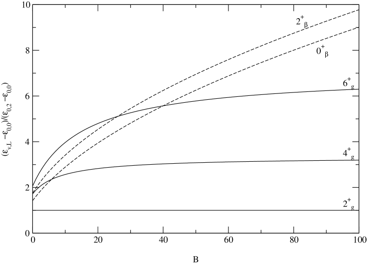
Figure 5: Reduced energies normalized to the energy difference between the first two states of the ground state band as a function of the parameter $B$. The first three states of the g.s. band $(v=0)$ as well as the first two of the $\beta-$band $(v=1)$ are displayed. One can notice that the beginning of the second band lies at higher energies when the deformation of the system is increased and eventually tends to infinity in the rotor limit.

Figure 6: Comparison between the calculated and experimental spectrum of ²³⁴U (positive parity states). The theoretical predictions are obtained according to (10) and (13) with the choice $B=393.7415$ and $c=-41.5629$ to define the $(\beta,\gamma)$ potential in (9) and (12). The ground state, $\beta$ and $\gamma$ bands are displayed.

For illustration we display in fig. 4 a section of a Kratzer potential along the line with $\gamma=0^{o}$. The parameters have been chosen to show how the well can be shaped in order to have a rotational behaviour in presence of a $\beta-$softness. In fact the position of some of the lowest states of the first two bands is quite deep in the well: this means that the variation of the mean square deformation will not change much among these states (so that the approximate separation of variables in eq. (1) is a posteriori justified). Note that the present solution requires only one parameter to fix the relative position of all the states in the lowest band and the position of the so-called $\beta-$bands (the parameter $A$ in the potential does not play any role in determining the scaled eigenvalues). The position of the $\gamma-$band is fixed by the additional parameter $c$ in eq. (13). As usual the physical values of the spectrum are then obtained by an overall scaling factor.
As we move to large deformations and deeper minima by increasing the parameter $B$, the position of the $\beta-$bands with respect to the ground state band moves higher in energy and a crossing occurs between the relative positions of states in different bands, as one can see in fig. 5.

We applied our form of the potential to describe the lowest rotational bands in ²³⁴U. A comparison between the lowest positive parity experimental energy levels of ²³⁴U [6] and the predictions of the model presented here are given in fig. 6. The agreement is good in spite of the fact that all the relative positions of the states in the ground state band and $\beta-$band have been fixed with only one parameter, $B$, that has been obtained fitting the energy of the $4_{g}^{+}$ level.

Note that, at variance with the experiment that seems to display almost equal moments of inertia for the ground and $\beta-$band, the theory gives a slightly larger moment for the $\beta-$band. This can be understood from the expansion of the general formula (10) in powers of $L(L+1)$. In leading order one obtains, for the energy differences within a generic band (characterized by the quantum number $v$), the following expression

$$\epsilon_{v,L}-\epsilon_{v,0}~{}=~{}L(L+1){A^{2}/24\over\sqrt{B+9/4}(\sqrt{B+9/4}+1/2+v)^{3}},$$ (18)

which leads to the mild dependence on $v$, discussed above.

In summary we have discussed a new solution of the Bohr hamiltonian with the aim of describing a $\beta-$soft, $\gamma-$soft axial rotor. We have given spectra and transition rates that may in principle encompass a broad range of situations and can be used to survey experimental data. We have discussed, as an example, the spectrum of ²³⁴U, that may be considered as a “quasi-rigid” rotor and that is accurately described within the present formalism, making use of the solution with a Kratzer-like potential.

References

References

• [1] L.Fortunato and A.Vitturi, J.Phys.G 29, 1341-1349 (2003).
• [2] F.Iachello, Phys.Rev.Lett. 85, 3580 (2000).
• [3] F.Iachello, Phys.Rev.Lett. 87, 052502 (2001).
• [4] D.M.Brink, Prog.Nucl.Phys. 8, 97 (1960).
• [5] Z.X.Wang and D.R.Guo, Special functions, World Scientific, Singapore (1989).
• [6] Isotope Explorer, LBNL-Lund Collaboration. http://ie.lbl.gov/ensdf/