The relation between the photonuclear E1 sum rule and the effective orbital g-factor

Abstract

The connection between the enhancement factor ($1+\kappa$) of the photonuclear E1 sum rule and the orbital angular momentum g-factor ($g_{\ell}$) of a bound nucleon is investigated in the framework of the Landau-Migdal theory for isospin asymmetric nuclear matter. Special emphasis is put on the role of gauge invariance to establish the $\kappa-g_{\ell}$ relation. By identifying the physical processes which are taken into account in $\kappa$ and $g_{\ell}$, the validity and limitations of this relation is discussed. The connections to the collective excitations and to nuclear Compton scattering are also shown.

1 Introduction

The enhancement factor ($1+\kappa$) of the photonuclear E1 sum rule and the orbital angular momentum g-factor ($g_{\ell}$) of a bound nucleon have attracted the attention of nuclear theorists as well as experimentalists for a long time, since these quantities reflect the presence of exchange forces and mesonic degrees of freedom in nuclei [1, 2, 3, 4]. More than 30 years ago, Fujita and Hirata [5] used the isospin symmetric Fermi gas as a model for an N=Z nucleus to derive the simple relation $1+\kappa=2\,g_{\ell,{\rm IV}}$ between $\kappa$ and the isovector (IV) part of $g_{\ell}$ in first order perturbation theory. Later it has been shown [6] that, because of the presence of correlations between the nucleons, only a part of the total $\kappa$ is related to $g_{\ell,{\rm IV}}$. It has been argued [7] that this part of $\kappa$ is related to the sum of the E1 strength in the region of the isovector giant dipole resonance (GDR). In more recent years [8], this modified $\kappa-g_{\ell}$ relation has been used to analyse the results of photo-neutron experiments [9] and photon scattering experiments [10, 11], in particular for nuclei in the lead region. In these analyses, the corrections to $g_{\ell,{\rm IV}}$ were associated with the meson exchange currents.

On the other hand, as early as 1965, Migdal and collaborators [12] used an approach based on a a gas of quasiparticles to relate $\kappa$ to the parameters characterizing the interaction between the quasiparticles (the Landau-Migdal parameters). Combining this relation with the more general one between $g_{\ell,{\rm IV}}$ and the Landau-Migdal parameters [13], their approach suggested that the relation $1+\kappa=2\,g_{\ell,{\rm IV}}$ holds more generally without recourse to perturbation theory. The fact that their result involves the total $\kappa$ instead of just a part of it reflects the quasiparticle gas approximation. Concerning the orbital g-factor, however, the Landau-Migdal approach suggests that it is the total $g_{\ell,{\rm IV}}$, and not only the part associated with the meson exchange currents, which enters in the relation to the E1 enhancement factor. By using a somewhat different approach, this result has also been obtained by Ichimura [14].

The main advantage of the Landau-Migdal theory [13], which is based on the Fermi liquid approach due to Landau [15, 16], is that symmetries, like gauge invariance and Galilei invariance, are incorporated rigorously, and that the description of the collective excitations of the system is physically very appealing. The Fermi liquid approach to discuss sum rules in nuclear matter has therefore turned out to be very fruitful, and has been used in several papers on giant resonances [17, 18]. However, to the best of our knowledge, a general discussion of the physical processes which contribute to the $\kappa$-$g_{\ell}$ relation, as well as a discussion on the physical origin of this relation, is still outstanding.

The strong interest in nuclear giant resonances and sum rules is continuing nowadays [19, 20], and new phenomena like the double giant resonances [21] or dipole resonances in neutron rich nuclei [22] have attracted attention. The Landau-Migdal theory, which is a strong candidate to describe the giant resonances [23], is now extended in various directions [24] so as to give a more general description which is valid up to higher excitation energies. In the light of these recent developments and the analyses of photonuclear experiments mentioned above, more detailed understanding on the $\kappa$-$g_{\ell}$ relation would be desirable.

In this paper we will present a general discussion on the $\kappa$-$g_{\ell}$ relation in isospin asymmetric nuclear matter, using the language of the Landau-Migdal theory. The aims of our work are as follows: First, we will extend the relations obtained previously for the orbital g-factor and the E1 enhancement factor to the case of $N\neq Z$, putting special emphasis on the role of gauge invariance. Second, we will identify the physical processes which are taken into account in the $\kappa$-$g_{\ell}$ relation, both in terms of Feynman diagrams as well as time-ordered Bethe-Goldstone diagrams. In this connection we will also discuss the relation to the collective excitations. Third, we will show the connection to the photon scattering amplitude, which establishes the physical origin of the $\kappa$-$g_{\ell}$ relation.

The rest of the paper is organized as follows: In sect. 2 we briefly review some relations of the Landau-Migdal theory which will be used for the discussions on $g_{\ell}$ and $\kappa$. In sect. 3 we derive the expressions for the proton and neutron orbital g-factors in isospin asymmetric nuclear matter, which are in principle exact and hold also in relativistic field theory. In sect. 4 we discuss the E1 sum rule and its relation to the orbital g-factors, limiting ourselves to the nonrelativistic case because of the problems associated with the center of mass motion. In sect. 5 we discuss the physical processes which are taken into account in the $\kappa-g_{\ell}$ relation and establish the connection to the collective excitations. In sect. 6 we discuss the relation to the nuclear Compton scattering amplitude, which provides the physical origin of the $\kappa$-$g_{\ell}$ relation. A summary and conclusions are given in sect. 7.

2 Vertices and correlation functions in the Landau-Migdal theory

In this section we briefly review some relations of the Landau-Migdal theory which will be used in later sections.

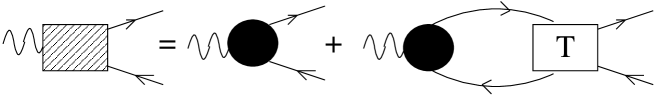
Figure 1: Graphical representation of relation (2.1) for the vertex. The shaded square stands for the full vertex ($\Gamma$), and the black circle for the vertex which is two-body irreducible in the p-h channel ($\Gamma_{0}$). $T$ denotes the $T$-matrix.

The integral equation for the electromagnetic vertex $\Gamma$ is graphically shown in Fig. 1 and is written symbolically as

$$\Gamma=\Gamma_{0}-i\,T\,S\,S\,\Gamma_{0},$$ (2.1)

where $\Gamma_{0}$ is the part which is two-body irreducible in the particle-hole (p-h) channel, $S$ is the full nucleon propagator, and $T$ is the two-body T-matrix which satisfies the Bethe-Salpeter equation

$$T=K-i\,T\,S\,S\,K$$ (2.2)

with the two-body irreducible kernel $K$. The important step in the renormalization procedure of the Landau-Migdal theory is to split the product $S\,S$ into the two parts [13]

$$S\,S\,=A\,+\,B,$$ (2.3)

where $A$ denotes the product of the pole parts of the particle and hole propagators (${\displaystyle A=S_{p}^{\rm(pole)}S_{h}^{\rm(pole)}}$), including the prescription to evaluate the other energy dependent quantities in a frequency loop integral for on-shell p-h states. (The explicit form of $A$ in the momentum representation will be specified below.) All other parts, like non-pole parts, the product of two particle or two hole propagators, antinucleon propagators etc, are included in the quantity $B$. The basic idea here is that the part $A$ represents the “active space”, while the effects of $B$ are renormalized into the effective vertex and effective interaction.

The equation (2.2) for the T-matrix is then equivalent to

$$T = T^{(\omega)}-i\,T\,A\,T^{(\omega)}$$ (2.4)

$$T^{(\omega)} = K-i\,T^{(\omega)}\,B\,K,$$ (2.5)

and equation (2.1) for the vertex is equivalent to

$$\Gamma = \Gamma^{(\omega)}-iT^{(\omega)}\,A\,\Gamma$$ (2.6)

$$\Gamma^{(\omega)} = \Gamma_{0}-iT^{(\omega)}\,B\,\Gamma_{0}.$$ (2.7)

As is clear from these equations, the quantities $T^{(\omega)}$ and $\Gamma^{(\omega)}$ do not involve the product $S_{p}^{\rm pole}S_{h}^{\rm pole}$ in the intermediate states, that is, they have no p-h cuts, and eqs. (2.4) and (2.6) can be considered as RPA-type equations with $T^{(\omega)}$ and $\Gamma^{(\omega)}$ playing the role of the effective interaction and the effective vertex, respectively, acting in the space of p-h states.

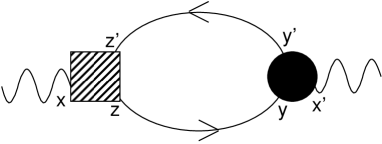
Figure 2: Graphical representation of eq.(2.8). For explanation of the symbols, see the caption to Fig.1.

Another quantity which is of particular interest for the collective excitations of the system is the electromagnetic current-current correlation function, or shortly the correlation function, which can be expressed in coordinate space as follows (see Fig.2) :

$$i\,\langle 0|T\left(j^{\mu}(x^{\prime})j^{\nu}(x)\right)|0\rangle=i\,{\rm Tr}\,\,\left[\Gamma_{0}^{\mu}(y,x^{\prime},y^{\prime})\,S(y^{\prime},z^{\prime})\,\Gamma^{\nu}(z^{\prime},x,z)\,S(z,y)\,\right],$$ (2.8)

or symbolically in the form

$$\Pi=i\,\Gamma_{0}\,S\,S\,\Gamma$$ (2.9)

The trace (${\rm Tr}$) in (2.8) stands for an integral over the space-time positions $z^{\prime},\,z,\,y^{\prime},\,y$ as well as the trace over spin-isospin indices.

If we use eqs. (2.3),  (2.6) and (2.7) in eq.(2.9), we obtain the separation of the correlation function into a part $\Pi_{A}$, which involves p-h cuts, and a part $\Pi_{B}$, which involves the rest, like $2p-2h$ cuts etc.:

$$\Pi=i\,\Gamma^{(\omega)}\,A\,\Gamma\,+\,i\,\Gamma_{0}\,B\,\Gamma^{(\omega)}\equiv\Pi_{A}+\Pi_{B}.$$ (2.10)

The use of eq.(2.6) for the vertex $\Gamma$ then generates the RPA series for the part $\Pi_{A}$.

For illustration, we represent $\Pi_{A}$ by Fig. 3, and show some selected examples for diagrams which contribute to $\Pi_{A}$ in Fig. 4.

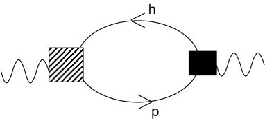
Figure 3: Graphical representation of the part $\Pi_{A}$ in eq.(2.10). The shaded square represents $\Gamma$, the black square $\Gamma^{(\omega)}$, and p (h) denotes the pole part of the particle (hole) propagator.

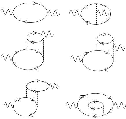
Figure 4: Some selected time-ordered diagrams contributing to $\Pi_{A}$. The first line shows the non-interacting part and a meson-exchange current contribution in first order perturbation theory, the second line shows some graphs which arise from 2p-2h states in the vertex $\Gamma^{(\omega)}$, and the third line shows some examples reflecting the 2p-2h states in the interaction $T^{(\omega)}$. The vertex where the external field couples to a dashed line stands symbolically for the two-body exchange currents. Self energy corrections also contribute, but are not shown in this figure.

The common feature of these diagrams is that they involve at least one electromagnetic vertex where a p-h pair is created by the external field. This is in contrast to the diagrams contributing exclusively to $\Pi_{B}$, for which we show some examples in Fig. 5.

Figure 5: Some selected time-ordered diagrams which contribute exclusively to $\Pi_{B}$.

We now specify the form of $A$ in momentum space, which corresponds to the product of the pole parts of particle and hole propagators:

$$S_{p}^{\rm(pole)}(k)=\frac{Z_{k}\,(1-n_{k})}{k_{0}-\epsilon_{k}+i\delta}\,,\,\,\,\,\,\,\,\,\,\,\,\,\,\,\,\,\,\,\,S_{h}^{\rm(pole)}(k)=\frac{Z_{k}\,n_{k}}{k_{0}-\epsilon_{k}-i\delta}\,,$$ (2.11)

where $\epsilon_{k}$ and $Z_{k}$ are the quasiparticle poles and residues, and $n_{k}$ is the Fermi distribution function. From the structure of the RPA-type equations (2.4) and (2.6) it is clear that each loop integral is associated with one factor $A$. We therefore consider the following expression to represent a generic loop integral which involves a p-h cut:

$${\cal I} = \int\frac{{\rm d}^{4}k}{(2\pi)^{4}}\left(S_{p}^{(\rm pole)}(k+\frac{q}{2})\,S_{h}^{(\rm pole)}(k-\frac{q}{2})+S_{h}^{(\rm pole)}(k+\frac{q}{2})\,S_{p}^{(\rm pole)}(k-\frac{q}{2})\right)$$ (2.12)

$$\times F(k+\frac{q}{2},k-\frac{q}{2})\,,$$

where $F$ does not contain $A$, and $q^{\mu}=(\omega,{\mbox{\boldmath${q}$}})$ is the momentum transferred by the external field. By closing the $k_{0}$ contour in the upper plane, we get

$${\cal I} = i\int\frac{{\rm d}^{3}k}{(2\pi)^{3}}\,Z_{k+}Z_{k-}\,\left(\frac{(1-n_{k+})n_{k-}}{\omega-(\epsilon_{k+}-\epsilon_{k-})+i\gamma}F\left((\omega+\epsilon_{k-})\,{\mbox{\boldmath${k}$}}_{+}\,;\,\epsilon_{k-}\,{\mbox{\boldmath${k}$}}_{-}\right)\right.$$ (2.13)

$$+ \left.\frac{n_{k+}(1-n_{k-})}{\omega-(\epsilon_{k+}-\epsilon_{k-})+i\gamma}F\left(\epsilon_{k+}\,{\mbox{\boldmath${k}$}}_{+}\,;\,(-\omega+\epsilon_{k+})\,{\mbox{\boldmath${k}$}}_{-}\right)\right)+{\cal I}_{F}\,\,,$$

where $\gamma\equiv\,$sign$\,\omega$, ${\cal I}_{F}$ denotes the contributions from the poles of $F$ in the upper plane, and all quantities with subindex ${k\pm}$ refer to the three momentum ${\mbox{\boldmath${k}$}}_{\pm}={\mbox{\boldmath${k}$}}\pm{\mbox{\boldmath${q}$}}/2$. We expand both functions $F$ in (2.13) around $\omega=\epsilon_{k+}-\epsilon_{k-}$, and take only the first term in this expansion. This, together with the prescription to omit the term ${\cal I}_{F}$, defines the quantity $A(k,q)$:

$${\cal I}_{A} = -i\int\frac{{\rm d}^{3}k}{(2\pi)^{3}}\,\frac{(n_{k+}-n_{k-})\,Z_{k+}Z_{k-}}{\omega-(\epsilon_{k+}-\epsilon_{k-})+i\gamma}\,F(\epsilon_{k+}\,{\mbox{\boldmath${k}$}}_{+}\,;\,\epsilon_{k-}\,{\mbox{\boldmath${k}$}}_{-})$$ (2.14)

$$\equiv \int\frac{{\rm d}^{4}k}{(2\pi)^{4}}\,A(k,q)\,F(k+\frac{q}{2},k-\frac{q}{2}).$$ (2.15)

From this identification we obtain

$$A(k,q)=-2\pi i\delta\left(k_{0}-\frac{\epsilon_{k+}+\epsilon_{k-}}{2}\right)\frac{(n_{k+}-n_{k-})\,Z_{k+}Z_{k-}}{\omega-(\epsilon_{k+}-\epsilon_{k-})+i\gamma}\,{\hat{P}}(\omega)\,,$$ (2.16)

where ${\hat{P}}(\omega)$ denotes the prescription to evaluate $F$ at $\omega=\epsilon_{k+}-\epsilon_{k-}$. Together with the delta function in (2.16) this means that $A$ effectively replaces the function ${\displaystyle F(k+\frac{q}{2},k-\frac{q}{2})}$ by its “on-shell” (o.s.) value defined by

$$k_{0}+\frac{\omega}{2}\stackrel{{\scriptstyle{\rm o.s.}}}{{=}}\epsilon_{k+},\,\,\,\,\,\,\,\,\,\,\,\,\,\,\,\,\,\,\,\,k_{0}-\frac{\omega}{2}\stackrel{{\scriptstyle{\rm o.s.}}}{{=}}\epsilon_{k-}.$$ (2.17)

Therefore, the contribution of a Feynman diagram, which has p-h cuts, to $\Pi_{A}$ is obtained by replacing the energy dependent vertices and T-matrices by their on-shell values. The rest is contained in $\Pi_{B}$. (Later we will specify what this means in terms of time-ordered Bethe-Goldstone diagrams, and make contact to the examples shown in Fig.4.)

A similar form of $A$ can be derived also in finite systems. In this case one uses the “$\lambda$-representation” [13] instead of the momentum representation, which involves a set of single particle wave functions $\Phi_{\lambda}(E)$ chosen so as to diagonalize the single particle Green function for fixed frequency $E$: $G_{\lambda^{\prime}\lambda}(E)=\delta_{\lambda^{\prime}\lambda}G_{\lambda}(E)$. The form of $A$ then becomes

$$A_{\lambda^{\prime}\lambda}(k_{0},\omega)=-2\pi i\delta\left(k_{0}-\frac{\epsilon_{\lambda^{\prime}}+\epsilon_{\lambda}}{2}\right)\frac{(n_{\lambda^{\prime}}-n_{\lambda})\,Z_{\lambda^{\prime}}Z_{\lambda}}{\omega-(\epsilon_{\lambda^{\prime}}-\epsilon_{\lambda})+i\gamma}\,{\hat{P}}(\omega)\,,$$ (2.18)

where ${\hat{P}}(\omega)$ implies to evaluate the function $F$, which appears in the same loop as $A$, at $\omega=\epsilon_{\lambda^{\prime}}-\epsilon_{\lambda}$.

Finally in this section, let us use the form (2.16) to write down the expression for $\Pi_{A}$ and the equation for $\Gamma$ in momentum space. For this purpose, we introduce the quasiparticle current $j^{(\omega)}$ and the quasiparticle interaction $t^{(\omega)}$ by

$$j^{(\omega)}(k_{+},k_{-}) \equiv \sqrt{Z_{k+}Z_{k-}}\,\,\Gamma^{(\omega)}(\epsilon_{k+}\,{\mbox{\boldmath${k}$}}_{+}\,;\,\epsilon_{k-}\,{\mbox{\boldmath${k}$}}_{-})$$ (2.19)

$$t^{(\omega)}(k_{+},k_{-};\ell_{+},\ell_{-}) \equiv \sqrt{Z_{k+}Z_{k-}Z_{\ell+}Z_{\ell-}}\,\,T^{(\omega)}(\epsilon_{k+}{\mbox{\boldmath${k}$}}_{+},\epsilon_{k-}{\mbox{\boldmath${k}$}}_{-};\epsilon_{\ell+}{\mbox{\boldmath${\ell}$}}_{+},\epsilon_{\ell-}{\mbox{\boldmath${\ell}$}}_{-})\,.$$

Defining also the total current $j(k_{+},k_{-})$ in terms of the total vertex $\Gamma$ in a way similar to (2.19), the expression for $\Pi_{A}$ can be written as

$$\Pi_{A}(\omega,{\mbox{\boldmath${q}$}})=V\,\int\frac{{\rm d}^{3}k}{(2\pi)^{3}}{\rm tr}\left(j^{(\omega)}(k_{-},k_{+})\,\frac{n_{k+}-n_{k-}}{\omega-(\epsilon_{k+}-\epsilon_{k-})+i\gamma}\,j(k_{+},k_{-})\right)$$

(2.21)

where $V$ is the volume of the system, and the equation for the current takes the form

$$j(k_{+},k_{-})=j^{(\omega)}(k_{+},k_{-})$$

$$-\int\frac{{\rm d}^{3}\ell}{(2\pi)^{3}}{\rm tr}\,\left[t^{(\omega)}(k_{+},k_{-};\ell_{+},\ell_{-})\,\frac{n_{\ell+}-n_{\ell-}}{\omega-(\epsilon_{\ell+}-\epsilon_{\ell-})+i\gamma}\,j(\ell_{+},\ell_{-})\right]\,.$$

Relations analogous to (2.21) and (LABEL:curr1) can also be written down for finite systems in the $\lambda$-representation.

3 The orbital g-factor

In this section we will extend the previously obtained relations [13, 26] for the orbital g-factor of a quasiparticle on the Fermi surface to the case of isospin asymmetric nuclear matter ($N\neq Z$). Although our notation will refer to the nonrelativistic case, the result is valid also in relativistic theories.

The magnetic moment associated with the quasiparticle current ${\mbox{\boldmath${j}$}}^{(\omega)}$ is obtained from ${\mbox{\boldmath${m}$}}=-\frac{i}{2}\left[{\mbox{\boldmath${\nabla}$}}_{q}\times\left({\mbox{\boldmath${j}$}}^{(\omega)}\delta^{(3)}({\mbox{\boldmath${p}$}}+{\mbox{\boldmath${q}$}}-{\mbox{\boldmath${p}$}}^{\prime})\right)\right]_{q=0}$. In nuclear matter, the only way to get a term proportional to the orbital angular momentum is to let the derivative act on the momentum conserving delta function [26]. Since the matrix element of the orbital angular momentum operator between plane wave states is $i{\mbox{\boldmath${p}$}}\times{\mbox{\boldmath${\nabla}$}_{p}}\delta^{(3)}({\mbox{\boldmath${p}$}}-{\mbox{\boldmath${p}$}}^{\prime})$, we obtain for the angular momentum g-factor of a proton or neutron at the Fermi surface

$$g_{\ell}(\alpha)=\frac{M}{e_{p}\cdot p_{F}(\alpha)}j^{(\omega)}_{\alpha}\,\,\,\,\,\,\,\,\,\,(\alpha=p,n)\,,$$ (3.1)

where $e_{p}>0$ is the proton electric charge, $p_{F}(p)$ and $p_{F}(n)$ denote the Fermi momenta of protons and neutrons, and the current $j^{(\omega)}_{\alpha}$ refers to the $q\rightarrow 0$ limit of the quasiparticle current (2.19) at the Fermi surface. The calculation of the angular momentum g-factor in nuclear matter therefore reduces to the calculation of the quasiparticle current at the Fermi surface at zero momentum transfer.

Invariance with respect to local gauge transformations of the charged particle fields leads to the Ward-Takahashi identity for the electromagnetic vertex, which in turn gives expressions for the currents $j_{\alpha}$ in the limit $\omega\rightarrow 0$ followed by $|{\mbox{\boldmath${q}$}}|\rightarrow 0$, which is called the “static limit”, following ref.[13]. (The use of the Ward-Takahashi identity in many-body systems has been explained in detail in refs. [26, 27] for relativistic theories, but for convenience we summarize some relations in Appendix A.) The results for the static limit of the proton and neutron currents are

$$j_{p}^{({\rm st})}=e_{p}\,v_{F}(p)\,,\,\,\,\,\,\,\,\,\,\,j_{n}^{({\rm st})}=0.$$ (3.2)

We denote by $v_{F}(\alpha)$ the Fermi velocities of protons ($\alpha=p$) and neutrons ($\alpha=n$).

Since we need the quasiparticle currents $j_{\alpha}^{(\omega)}$ instead of the static currents $j_{\alpha}^{({\rm st})}$, we have to use eq.(LABEL:curr1) in the limit$\omega\rightarrow 0$ followed by $|{\mbox{\boldmath${q}$}}|\rightarrow 0$. In this limit, we can use

$$\frac{n_{\ell+}-n_{\ell-}}{\omega-(\epsilon_{\ell+}-\epsilon_{\ell-})+i\gamma}\Rightarrow\frac{1}{v_{F}}\delta(|{\mbox{\boldmath${\ell}$}}|-p_{F})$$ (3.3)

for either protons or neutrons. Then both vectors ${k}$ and ${\ell}$ in eq.(LABEL:curr1) are on the Fermi surface, and the integral reduces to an integral over the angle between the directions ${\hat{\mbox{\boldmath${k}$}}}$ and ${\hat{\mbox{\boldmath${\ell}$}}}$ (Landau angle). In this kinematics, the interaction $t^{(\omega)}$ depends only on the Landau angle and becomes the “Landau-Migdal interaction”. It is convenient to introduce the dimensionless interaction

$${\cal F}({\hat{\mbox{\boldmath${k}$}}}\cdot{\hat{\mbox{\boldmath${\ell}$}}})\equiv\frac{2p_{F}^{2}}{\pi^{2}}\,\frac{1}{v_{F}}\,t^{(\omega)}({\hat{\mbox{\boldmath${k}$}}}\cdot{\hat{\mbox{\boldmath${\ell}$}}})\,,$$ (3.4)

where by definition we identify $p_{F}$ and $v_{F}$ with the Fermi momentum and the Fermi velocity in symmetric nuclear matter with the same baryon density. It is then easy to obtain the following relations from eq.(LABEL:curr1) and (3.2) (see Appendix A):

$$j_{p}^{(\omega)} = e_{p}\left[v_{F}(p)+\frac{v_{F}}{6}\left(\frac{p_{F}(p)}{p_{F}}\right)^{2}F_{1}(pp)\right]$$ (3.5)

$$j_{n}^{(\omega)} = e_{p}\,\frac{v_{F}}{6}\left(\frac{p_{F}(p)}{p_{F}}\right)^{2}F_{1}(pn)\,,$$ (3.6)

where $F_{1}(pp)$ and $F_{1}(pn)=F_{1}(np)$ are the coefficients of the $\ell=1$ Legendre polynomials $P_{1}({\hat{\mbox{\boldmath${k}$}}}\cdot{\hat{\mbox{\boldmath${\ell}$}}})$ in an expansion of the spin-independent part of ${\cal F}_{pp}$ or ${\cal F}_{pn}$ . Lorentz invariance, or Galilei invariance in the nonrelativistic case, can then be used (see Appendix A) to rewrite these expressions in the form

$$j^{(\omega)}_{p} = e_{p}\left[\frac{p_{F}(p)}{\mu_{p}}-\frac{p_{F}(p)v_{F}}{6p_{F}}F_{1}(pn)\frac{\mu_{n}}{\mu_{p}}\left(\frac{p_{F}(n)}{p_{F}}\right)^{3}\,\beta\right]$$ (3.7)

$$j^{(\omega)}_{n} = e_{p}\,\frac{p_{F}(n)v_{F}}{6p_{F}}F_{1}(pn)\left(\frac{p_{F}(p)}{p_{F}}\right)^{3}\,\beta\,,$$ (3.8)

where $\mu_{p}$ and $\mu_{n}$ are the chemical potentials (Fermi energies including the rest masses) of protons and neutrons, and

$$\beta\equiv\frac{p_{F}^{2}}{p_{F}(p)p_{F}(n)}=\left[1-\left(\frac{N-Z}{A}\right)^{2}\right]^{-\frac{1}{3}}$$ (3.9)

The orbital g-factors then can be expressed as follows :

$$g_{\ell}(p) = \frac{M}{\mu_{p}}-\frac{Mv_{F}}{3p_{F}}\,F_{1}(pn)\,\frac{\mu_{n}}{\mu_{p}}\,\frac{N}{A}\,\beta$$ (3.10)

$$g_{\ell}(n) = \frac{Mv_{F}}{3p_{F}}\,F_{1}(pn)\,\frac{Z}{A}\,\beta\,.$$ (3.11)

We note that the following relation holds between the proton and neutron orbital g-factors:

$$\frac{Z}{A}\,\frac{\mu_{p}}{M}\,g_{\ell}(p)+\frac{N}{A}\,\frac{\mu_{n}}{M}\,g_{\ell}(n)=\frac{Z}{A}\,.$$ (3.12)

In a nonrelatistic theory we have $\mu_{p}=\mu_{n}=M$, and eq. (3.12) is the extension to $N\neq Z$ of the well known fact [26, 27] that the isoscalar orbital g-factor is renormalized exclusively by relativistic effects.

Besides the dependence on the neutron excess shown explicitly in (3.10) and (3.11), the Landau-Migdal parameter $F_{1}(pn)$ might also depend on $(N-Z)/A$ for fixed $A$. If the range of the interaction is small compared to $1/p_{F}$, this dependence can be expected to be weak. For the case of the long range 1-pion exchange interaction, we note that in $F_{1}(pn)$ the average over the cosine of the Landau angle ($\cos\Theta_{L}\equiv x$) is performed with respect to the momentum transfer in the exchange channel, which is ${\mbox{\boldmath${Q}$}}^{2}=\left({\mbox{\boldmath${k}$}}-{\mbox{\boldmath${\ell}$}}\right)^{2}=p_{F}(p)^{2}+p_{F}(n)^{2}-2p_{F}(p)p_{F}(n)x=2p_{F}^{2}(1-x)+{\cal O}\left[\left(\frac{N-Z}{3A}\right)^{2}\right]$. Therefore, up to ${\cal O}\left(\frac{N-Z}{A}\right)$, the dependence on the neutron excess is as shown by the explicit factors $N/A$ and $Z/A$ in the relations (3.10) and (3.11).

4 The E1 sum rule and the $\kappa-g_{\ell}$ relation

While the treatment of the orbital g-factor in the previous section was completely general, the discussion of the E1 sum rule is plagued by problems related to the spurious center of mass motion [25]. Therefore, from now we have to restrict ourselves to a nonrelativistic framework, and consider the case of a Hamiltonian

$${\hat{H}} = \frac{-1}{2M}\int{\rm d}^{3}r\,\,\psi^{\dagger}({\mbox{\boldmath${r}$}})\,\Delta\,\psi({\mbox{\boldmath${r}$}})$$ (4.1)

$$+ \frac{1}{2}\int{\rm d}^{3}r_{1}\int{\rm d}^{3}r_{2}\,\,\psi^{\dagger}({\mbox{\boldmath${r}$}}_{1})\psi^{\dagger}({\mbox{\boldmath${r}$}}_{2})\,V({\mbox{\boldmath${r}$}}_{1},{\mbox{\boldmath${r}$}}_{2})\,\psi({\mbox{\boldmath${r}$}}_{2})\psi({\mbox{\boldmath${r}$}}_{1})$$ (4.2)

$$\equiv {\hat{H}}_{0}+{\hat{V}}$$ (4.3)

with the two-body potential

$$V({\mbox{\boldmath${r}$}}_{1},{\mbox{\boldmath${r}$}}_{2})=V_{0}({\mbox{\boldmath${r}$}}_{1},{\mbox{\boldmath${r}$}}_{2})+{\mbox{\boldmath${\tau}$}}_{1}\cdot{\mbox{\boldmath${\tau}$}}_{2}\,V_{1}({\mbox{\boldmath${r}$}}_{1},{\mbox{\boldmath${r}$}}_{2}).$$ (4.4)

4.1 Effective charges and gauge invariance

In this subsection, we digress to a discussion of local gauge invariance of a Hamiltonian containing two-body potentials. Our aims are, first, to investigate whether the introduction of the familiar E1 effective charges, which eliminate the spurious center of mass motion, is consistent with gauge invariance, and, second, derive some relations for the 2-body part of the electromagnetic interaction which will be used later.

Let us consider local gauge transformations of the form

$$\psi({\mbox{\boldmath${r}$}})\rightarrow{\rm exp}\left[i{\hat{Q}}\chi({\mbox{\boldmath${r}$}})\right]\,\psi({\mbox{\boldmath${r}$}})$$ (4.5)

where $\chi({\mbox{\boldmath${r}$}})$ is the gauge function, and

$${\hat{Q}}\equiv\frac{1+\tau_{z}}{2}\,Q_{p}+\frac{1-\tau_{z}}{2}\,Q_{n}\,.$$ (4.6)

In the first place, of course, we take the physical electric charges $e_{p}=-e>0$ and $e_{n}=0$ for $Q_{p}$ and $Q_{n}$, but we wish to keep our expressions more general in order to incorporate the effective charges in the later discussions. This gauge transformation effectively changes the first quantized operators as follows:

$$H_{0}(i) \rightarrow {\rm exp}\left[-i{\hat{Q}}^{(i)}\chi_{i}\right]H_{0}(i)\left[i{\hat{Q}}^{(i)}\chi_{i}\right]$$ (4.7)

$$V(i,j) \rightarrow {\rm exp}\left[-i\left({\hat{Q}}^{(i)}\chi_{i}+{\hat{Q}}^{(j)}\chi_{j}\right)\right]V(i,j)\left[i\left({\hat{Q}}^{(i)}\chi_{i}+{\hat{Q}}^{(j)}\chi_{j}\right)\right],$$

where $\chi_{i}\equiv\chi({\mbox{\boldmath${r}$}}_{i})$, $\chi_{j}\equiv\chi({\mbox{\boldmath${r}$}}_{j})$, and the other notations are self evident. Although it is not difficult to work out these expressions for a general gauge function, we consider here the long wave length limit (LWL) limit in order to derive the necessary relations most directly. In this case it is sufficient to consider $\chi({\mbox{\boldmath${r}$}})=c_{0}+{\mbox{\boldmath${r}$}}\cdot{\mbox{\boldmath${c}$}}$, where the $c_{\alpha}$ are constants. Using the fact that the 2-body potential commutes with the total 2-body isospin operator, the quantity $\left({\hat{Q}}^{(i)}\chi_{i}+{\hat{Q}}^{(j)}\chi_{j}\right)$ in the gauge transformation (LABEL:th1) can be replaced by ${\mbox{\boldmath${c}$}}\cdot\left({\mbox{\boldmath${D}$}}_{Q}^{(i)}+{\mbox{\boldmath${D}$}}_{Q}^{(j)}\right)$, where ${\mbox{\boldmath${D}$}}_{Q}^{(i)}={\hat{Q}}^{(i)}{\mbox{\boldmath${r}$}}_{i}$ is the dipole operator for particle $i$, referring to arbitrary charges $Q_{p}$ and $Q_{n}$. Since also (4.7) can be expressed by the dipole operator for particle $i$, the gauge transformation of the total Hamiltonian in first quantization

$$H=H_{0}+V\equiv\sum_{i}H_{0}(i)+\sum_{i<j}V(i,j)$$ (4.9)

can be written in terms of the dipole operator ${\displaystyle{\mbox{\boldmath${D}$}}_{Q}=\sum_{i}{\mbox{\boldmath${D}$}}_{Q}^{(i)}}$ as follows:

$$H\rightarrow{\rm exp}\left[-i{\mbox{\boldmath${c}$}}\cdot{\mbox{\boldmath${D}$}}_{Q}\right]\,H\,{\rm exp}\left[i{\mbox{\boldmath${c}$}}\cdot{\mbox{\boldmath${D}$}}_{Q}\right]\,.$$ (4.10)

This expression can be expanded in a series of multi-commutators:

$$H\rightarrow H-i{\mbox{\boldmath${c}$}}\cdot\left[{\mbox{\boldmath${D}$}}_{Q},H\right]-\frac{1}{2}c^{i}c^{j}\left[D^{i}_{Q},\left[D^{j}_{Q},H\right]\right]+\dots$$ (4.11)

where we have shown the terms up to ${\cal O}(e^{2})$ explicitly. The Hamiltonian can then be made locally gauge invariant up to some power of $e$ by introducing the gauge (photon) field ${A}$ which transforms under the gauge transformation as ${\mbox{\boldmath${A}$}}\rightarrow{\mbox{\boldmath${A}$}}+{\mbox{\boldmath${\nabla}$}}\chi$. It is then straight forward (see Appendix B) to show that the following Hamiltonian is locally gauge invariant up to ${\cal O}(e^{2})$:

$${\cal H}(Q_{p},Q_{n}) = H+i{\mbox{\boldmath${A}$}}\cdot\left[{\mbox{\boldmath${D}$}}_{Q},H\right]-\frac{1}{2}A^{i}A^{j}\left[D^{i}_{Q},\left[D^{j}_{Q},H\right]\right]$$ (4.12)

$$\equiv H+\delta H_{0}(Q_{p},Q_{n})+\delta V(Q_{p},Q_{n}),$$ (4.13)

where $\delta H_{0}$ ($\delta V$) is the contribution from $H_{0}$ ($V$) to the commutator terms. Evaluating the part $\delta H_{0}$ explicitly, we arrive at the familiar form

$${\cal H}(Q_{p},Q_{n})=\frac{1}{2M}\sum_{i=1}^{Z}\left({\mbox{\boldmath${p}$}}_{i}-Q_{p}{\mbox{\boldmath${A}$}}\right)^{2}+\frac{1}{2M}\sum_{i=1}^{N}\left({\mbox{\boldmath${p}$}}_{i}-Q_{n}{\mbox{\boldmath${A}$}}\right)^{2}+\delta V(Q_{p},Q_{n})\,,$$

(4.14)

where

$$\delta V(Q_{p},Q_{n})=i{\mbox{\boldmath${A}$}}\cdot\left[{\mbox{\boldmath${D}$}}_{Q},V\right]-\frac{1}{2}A^{i}A^{j}\left[D_{Q}^{i},\left[D_{Q}^{j},V\right]\right]\,.$$ (4.15)

The second term on the r.h.s. of (4.12) involves the familiar form of the current operator in the LWL: ${\mbox{\boldmath${j}$}}_{Q}({\mbox{\boldmath${q}$}}=0)=i[H,{\mbox{\boldmath${D}$}}_{Q}]$. The third term on the r.h.s. involves the 2-body part of the Compton scattering amplitude in the LWL, as will be discussed in more detail in sect. 6.

Here we note the following point concerning the dependence of the interaction term $\delta V$ on the charges $Q_{p}$ and $Q_{n}$: If we consider a pair of nucleons denoted by $(1,2)$, the relevant term in the dipole operator is

$${\mbox{\boldmath${D}$}}_{Q,12}={\hat{Q}}^{(1)}{\mbox{\boldmath${r}$}}_{1}+{\hat{Q}}^{(2)}{\mbox{\boldmath${r}$}}_{2}={\mbox{\boldmath${R}$}}\left(Q+T_{z}\,\Delta Q\right)+\frac{\mbox{\boldmath${r}$}}{4}\,\Delta Q\,\left(\tau_{z}^{(1)}-\tau_{z}^{(1)}\right),$$ (4.16)

where ${R}$ and ${r}$ are the c.m. and relative coordinates of the pair $(1,2)$, $T_{z}=\left(\tau_{z}^{(1)}+\tau_{z}^{(1)}\right)/2$, and $Q\equiv Q_{p}+Q_{n}$, $\Delta Q\equiv Q_{p}-Q_{n}$. Using this expression in (4.15), we see that, if the potential commutes with the 2-body c.m. coordinate ($\left[V,{\mbox{\boldmath${R}$}}\right]=0$), the 2-body current (first term on the r.h.s. of eq.(4.15)) depends only on the difference of the charges $\Delta Q$ and not on the sum $Q$. From the Jacobi identity for double commutators it is seen that the same holds also for the two-body part of the photon scattering amplitude (second term on the r.h.s. of eq.(4.15)) . This is important for our later discussions, since the effective charges for E1 transitions, $q_{p}=e_{p}\,N/A$, $q_{n}=-e_{p}\,Z/A$, satisfy $\Delta q=e_{p}$ as do the physical electric charges. Therefore, if the two-body potential commutes with the two-body c.m. coordinate, the interaction terms in the Hamiltonian (4.14) are invariant under the replacement of the physical charges are by the effective ones: $\delta V(q_{p},q_{n})=\delta V(e_{p},e_{n})$.

The introduction of the effective charges is then done as usual: First, for the physical charges we have

$${\cal H}(e_{p},e_{n})=H_{0}-\frac{e_{p}}{M}\sum_{i=1}^{Z}{\mbox{\boldmath${p}$}}_{i}\cdot{\mbox{\boldmath${A}$}}+\frac{e_{p}^{2}}{2M}\sum_{i=1}^{Z}{\mbox{\boldmath${A}$}}^{2}+\delta V(e_{p},e_{n})\,.$$ (4.17)

Second, in order to remove the effect of the center of mass motion on the electromagnetic interaction, we replace the momenta ${\mbox{\boldmath${p}$}}_{i}$ in the second term of (4.17) by the Jacobi momenta ${\mbox{\boldmath${p}$}}_{i}-{\mbox{\boldmath${P}$}}/A$, where ${\mbox{\boldmath${P}$}}=\sum_{i}{\mbox{\boldmath${p}$}}_{i}$ is the total momentum [37]. This replacement naturally leads to the effective charges

$$q_{p}=\frac{N}{A}\,e_{p}\,,\,\,\,\,\,\,\,\,\,\,\,\,q_{n}=-\frac{Z}{A}\,e_{p}\,.$$ (4.18)

Third, since ${A}$ is a constant in the LWL considered here, we can use the following identity for the third term on the r.h.s. of (4.17):

$$Ze_{p}^{2}=\frac{Z^{2}e_{p}^{2}}{A}+Zq_{p}^{2}+Nq_{n}^{2}$$ (4.19)

to obtain the final form of the Hamiltonian as

$${\hat{\cal H}}(q_{p},q_{n})=\frac{Z^{2}e_{p}^{2}}{2MA}\,{\mbox{\boldmath${A}$}}^{2}+{\cal H}(q_{p},q_{n}).$$ (4.20)

Here the first term describes the Thomson scattering of the nucleus as a whole [25], and ${\cal H}(q_{p},q_{n})$ is given by (4.14) with the effective charges (4.18).

The procedure to remove the c.m. motion therefore leads to the Hamiltonian ${\cal H}(q_{p},q_{n})$, which is locally gauge invariant under the gauge transformation involving the effective charges. Therefore one can continue to use all consequences of local gauge invariance, like Ward identities etc., for the theory described by the Hamiltonian ${\cal H}(q_{p},q_{n})$.

4.2 The E1 sum rule

The strength function (cross section) for the absorption of unpolarized photons by a nucleus in its ground state $|0\rangle$ is given by [25]

$$S(\omega) = 4\pi^{2}\sum_{n}|\langle n|{\hat{j}}({\mbox{\boldmath${q}$}})\frac{1}{\sqrt{\omega}}|0\rangle|^{2}\,\delta(\omega-\omega_{n0})$$ (4.21)

$$\stackrel{{\scriptstyle\rm LWL}}{{\longrightarrow}} 4\pi^{2}\sum_{n}|\langle n|{\hat{j}}({\mbox{\boldmath${q}$}}=0)\frac{1}{\sqrt{\omega}}|0\rangle|^{2}\,\delta(\omega-\omega_{n0}),$$ (4.22)

where ${\hat{j}}({\mbox{\boldmath${q}$}})$ denotes the Fourier transform of the 3-component (or any other space component) of the electromagnetic current operator for the effective charges (4.18), and $\omega_{n0}=E_{n}-E_{0}$ is the excitation energy of the state $|n\rangle$. The factor $\frac{1}{\sqrt{\omega}}$ in (4.21) and (4.22) originates from the normalization of the photon field. The LWL indicated in (4.22) holds if $|{\mbox{\boldmath${q}$}}|R<<1$, where $R$ is the nuclear radius.

In the LWL one can use current conservation to express the current operator as ${\hat{j}}({\mbox{\boldmath${q}$}}=0)=i[H,D_{q}]$, where $D_{q}$ is the 3-component of the dipole operator involving the effective charges (4.18). Then one arrives at the “nonretarded” E1 sum rule [25]

$$S\equiv\int_{0}^{\infty}{\rm d}\omega\,S(\omega) = 4\pi^{2}\sum_{n}\frac{1}{\omega_{n0}}\,|\langle n|{\hat{j}}({\mbox{\boldmath${q}$}}=0)|0\rangle|^{2}$$ (4.23)

$$= -2\pi^{2}\langle 0|\left[\left[H,D_{q}\right],D_{q}\right]|0\rangle.$$ (4.24)

Of course, this sum rule is not directly observable, since it includes only the unretarded E1 multipole, and for high $\omega$ ($=|{\mbox{\boldmath${q}$}}|$ for a physical photon) the LWL is not valid. It is therefore important to identify a part of the sum rule which holds in the low energy region where the LWL is justified.

We now relate the strength function and sum rule to the Fourier transform of the correlation function (see eq. (2.8))

$$\Pi^{\mu\nu}({\mbox{\boldmath${q}$}}^{\prime},{\mbox{\boldmath${q}$}};\omega)=i\int_{-\infty}^{\infty}{\rm d}\tau\,e^{i\omega\tau}\langle 0|T\left({\hat{j}}^{\mu}({\mbox{\boldmath${q}$}}^{\prime},t^{\prime}){\hat{j}}^{\nu}(-{\mbox{\boldmath${q}$}},t)\right)|0\rangle,$$ (4.25)

where $\tau=t^{\prime}-t\,$, and ${q}$ and ${\mbox{\boldmath${q}$}}^{\prime}$ are the incoming and outgoing momenta. For the case of forward scattering we define $\Pi^{\mu\nu}({\mbox{\boldmath${q}$}},\omega)\equiv\Pi^{\mu\nu}({\mbox{\boldmath${q}$}},{\mbox{\boldmath${q}$}};\omega)$, and obtain from eq.(4.25) the spectral representation for the 33-component

$$\Pi({\mbox{\boldmath${q}$}},\omega)=-\sum_{n}|\langle 0|{\hat{j}}({\mbox{\boldmath${q}$}})|n\rangle|^{2}\left(\frac{1}{\omega-\omega_{n0}+i\delta}-\frac{1}{\omega+\omega_{n0}-i\delta}\right).$$ (4.26)

Comparison with eqs. (4.21) and (4.23) gives

$$S(\omega) = \frac{4\pi}{\omega}\,\,{\rm Im}\,\Pi({\mbox{\boldmath${q}$}}=0,\omega)\,\,\,\,\,\,\,\,\,\,\,\,\,\,\,(\omega>0)$$ (4.27)

$$S = 2\pi^{2}\,\,\Pi({\mbox{\boldmath${q}$}}=0,\omega=0).$$ (4.28)

So far, all relations of this subsection hold for finite nuclei. The strength function in the LWL, eq. (4.27), is actually meaningless in nuclear matter, since there is no scale which corresponds to the nuclear radius $R$. The sum rule (4.28), however, represents a bulk property of the nucleus which should not depend on the details of nuclear structure, and therefore the discussion of the sum rule in nuclear matter has been the subject of many previous investigations [3]-[7].

In order to apply eq.(4.28) in nuclear matter and to discuss the $\kappa$-$g_{\ell}$ relation, we have to know the order in which the limits ${\mbox{\boldmath${q}$}}\rightarrow 0,\,\,\omega\rightarrow 0$ should be taken. This is important, because if ${\mbox{\boldmath${q}$}}\rightarrow 0$ is taken first (the “$\omega$-limit” of sect. 3), the p-h excitations do not contribute to the polarization, while for $\omega\rightarrow 0$ first (the “static limit”) they contribute at the Fermi surface [26]. We therefore present an alternative derivation of eq.(4.28), which makes clear the order of the limits. We make use of the following identity [38]:

$$\frac{\partial}{\partial x^{\prime\mu}}\,\frac{\partial}{\partial x^{\nu}}\langle 0|T\left({\hat{j}}^{\mu}(x^{\prime})\,{\hat{j}}^{\nu}(x)\right)|0\rangle=-\langle 0|\left[{\hat{j}}^{0}(x^{\prime}),{\hat{j}}^{0}(x)\right]|0\rangle\left(\frac{\partial}{\partial\tau}\,\,\delta\left({\tau}\right)\right).$$ (4.29)

The use of a partial integration in $\tau$ and the Heisenberg equation of motion for ${\hat{j}}^{0}$ then gives the following Ward-Takahashi identity for the correlation function (4.25):

$$q^{\prime}_{\mu}q_{\nu}\Pi^{\mu\nu}({\mbox{\boldmath${q}$}}^{\prime},{\mbox{\boldmath${q}$}};\omega)=-\langle 0|\left[\left[H,{\hat{j}}^{0}(-{\mbox{\boldmath${q}$}})\right],{\hat{j}}^{0}({\mbox{\boldmath${q}$}}^{\prime})\right]|0\rangle+\omega\,\,\langle 0|\left[{\hat{j}}^{0}(-{\mbox{\boldmath${q}$}}),{\hat{j}}^{0}({\mbox{\boldmath${q}$}}^{\prime})\right]|0\rangle$$ (4.30)

where $q^{\prime\mu}=(\omega,{\mbox{\boldmath${q}$}}^{\prime})$ and $q^{\mu}=(\omega,{\mbox{\boldmath${q}$}})$. We set $\omega=0$ in this identity, then apply ${\displaystyle\frac{\partial}{\partial q^{\prime}_{i}}\,\frac{\partial}{\partial q_{j}}}$ to both sides, and finally let ${\mbox{\boldmath${q}$}^{\prime}}$ and ${q}$ go to zero to obtain the low-energy theorem

$$\Pi({\mbox{\boldmath${q}$}}=0,\omega=0)=-\langle 0|\left[\left[H,D_{q}\right],D_{q}\right]|0\rangle,$$ (4.31)

where now the limit is defined as $\omega\rightarrow 0$ first followed by ${\mbox{\boldmath${q}$}}\rightarrow 0$ (“static limit”). Comparison with eq. (4.24) then gives again the relation (4.28) with this particular “static limit” prescription for the low frequency / low wave length limit.

Comparison with eq.(4.12) of the previous section shows that the double commutator in (4.31), which determines the sum rule (4.24), is the “seagull part” of the low energy photon scattering amplitude. This point will be further discussed in sect. 6.

4.3 The $\kappa-g_{\ell}$ relation

The polarization, which determines the sum rule by (4.28), has been split into two parts in eq.(2.10). We will now show that the part $\Pi_{A}$, which has been given explicitly in (2.21), is related to the orbital g-factors. The part $\Pi_{B}$, on the other hand, has no relation to the g-factors.

Taking the static limit ($\omega\rightarrow 0$ first, then ${\mbox{\boldmath${q}$}}\rightarrow 0$) of $\Pi_{A}$ in (2.21), we obtain

$$\Pi_{A}(\omega=0,{\mbox{\boldmath${q}$}}=0)={\hat{j}}^{(\omega)}_{p}\frac{Z}{v_{F}(p)p_{F}(p)}{\hat{j}}_{p}^{({\rm st})}+{\hat{j}}^{(\omega)}_{n}\frac{N}{v_{F}(n)p_{F}(n)}{\hat{j}}_{n}^{({\rm st})}\,,$$ (4.32)

where the currents ${\hat{j}}^{(\omega)}$ and ${\hat{j}}^{({\rm st})}$ at the Fermi surface refer to the effective charges, in contrast to the currents for the physical charges used in sect.3.

We now follow the same steps as in sect. 3: The Ward identities determine the currents in the static limit as

$${\hat{j}}_{p}^{({\rm st})}=q_{p}v_{F}(p)\,,\,\,\,\,\,\,\,\,\,\,{\hat{j}}_{n}^{({\rm st})}=q_{n}v_{F}(n).$$ (4.33)

Relation (LABEL:curr1) then gives the currents in the $\omega$-limit:

$${\hat{j}}_{p}^{(\omega)} = q_{p}\left[v_{F}(p)+\frac{v_{F}}{6}\left(\frac{p_{F}(p)}{p_{F}}\right)^{2}F_{1}(pp)\right]+q_{n}\frac{v_{F}}{6}\left(\frac{p_{F}(n)}{p_{F}}\right)^{2}F_{1}(pn)$$

$${\hat{j}}_{n}^{(\omega)} = q_{n}\left[v_{F}(n)+\frac{v_{F}}{6}\left(\frac{p_{F}(p)}{p_{F}}\right)^{2}F_{1}(nn)\right]+q_{p}\frac{v_{F}}{6}\left(\frac{p_{F}(p)}{p_{F}}\right)^{2}F_{1}(pn)\,.$$

If we use the Landau effective mass relations of Appendix A for the nonrelativistic case, we obtain the very simple results

$${\hat{j}}_{p}^{(\omega)}=j_{p}^{(\omega)}-Ze_{p}\,\frac{p_{F}(p)}{AM}\,,\,\,\,\,\,\,\,\,\,\,\,\,\,\,\,\,\,\,\,\,{\hat{j}}_{n}^{(\omega)}=j_{n}^{(\omega)}-Ze_{p}\,\frac{p_{F}(n)}{AM}\,,$$ (4.36)

where the currents $j_{p}^{(\omega)}$ and $j_{n}^{(\omega)}$ for the physical charges are given by eqs. (3.7) and (3.8) in the nonrelativistic limit $\mu_{p}=\mu_{n}=M$. The relations (4.36) clearly show the role of the effective charges to remove the c.m. motion: For the case $N=Z$ the subtractions in (4.36) make sure that there are no contributions from isoscalar currents to the collective motion of the system.

Inserting the static currents (4.33) and the $\omega$-currents (4.36) into (4.32), and using the definition of the orbital g-factors (3.1), we obtain

$$\Pi_{A}(\omega=0,{\mbox{\boldmath${q}$}}=0)=e_{p}^{2}\frac{NZ}{AM}\left(g_{\ell}(p)-g_{\ell}(n)\right).$$ (4.37)

The sum rule (4.28) then can be expressed as

$$S=({\rm TRK})\left(1+\kappa_{A}+\kappa_{B}\right)\equiv S_{A}+S_{B}\,,$$ (4.38)

where ${\displaystyle({\rm TRK})=2\pi^{2}e_{p}^{2}\frac{NZ}{AM}}$ is the Thomas-Reiche-Kuhn sum rule value, and the enhancement factor $1+\kappa$ has been split into the two parts $1+\kappa_{A}$ and $\kappa_{B}$ originating from $\Pi_{A}$ and $\Pi_{B}$, respectively:

$$1+\kappa_{A} = \frac{1}{e_{p}^{2}}\frac{AM}{NZ}\,\Pi_{A}({\mbox{\boldmath${q}$}}=0,\omega=0)=g_{\ell}(p)-g_{\ell}(n)$$ (4.39)

$$\kappa_{B} = \frac{1}{e_{p}^{2}}\frac{AM}{NZ}\,\Pi_{B}({\mbox{\boldmath${q}$}}=0,\omega=0).$$ (4.40)

Using (3.12), the relation (4.39) between $\kappa_{A}$ and the orbital g-factors can also be expressed as follows:

$$g_{\ell}(p) = 1+\frac{N}{A}\kappa_{A}$$ (4.41)

$$g_{\ell}(n) = -\frac{Z}{A}\kappa_{A}\,,$$ (4.42)

where $\kappa_{A}$ is given by

$$\kappa_{A}=-\frac{Mv_{F}}{3\,p_{F}}\,F_{1}(pn)\,\left[1-\left(\frac{N-Z}{A}\right)^{2}\right]^{-\frac{1}{3}}.$$ (4.43)

From our discussions in sect. 3 concerning the dependence of $F_{1}(pn)$ on the neutron excess, we see that the deviation of $\kappa_{A}$ from its value for symmetric nuclear matter starts with $\left((N-Z)/A\right)^{2}$.

5 Discussion

As we pointed out in sect.3, the expressions (3.10) and (3.11) are exact in nuclear matter and therefore take into account all possible contributions from meson exchange currents and configuration mixings, except for the conventional RPA-type contributions (e.g., the first order configuration mixing). The E1 enhancement factor $\kappa$, on the other hand, has been split into the pieces $\kappa_{A}$ and $\kappa_{B}$ in eq.(4.38), and only $\kappa_{A}$ is related to the orbital g-factors. In this section we wish to discuss which processes are taken into account by $\kappa_{A}$, and whether $\kappa_{A}$ can be related to the experimentally measured sum rule.

For this purpose, we return to eq.(2.10), where the polarization has been split into the two pieces $\Pi_{A}$ and $\Pi_{B}$. According to the optical theorem (4.27), the strength function for finite nuclei in the LWL then splits into two pieces as well: $S(\omega)=S_{A}(\omega)+S_{B}(\omega)$. We first wish to discuss the piece $\Pi_{A}$ in terms of Bethe-Goldstone diagrams. From the structure of eqs. (2.6), (2.10), and the energy denominator appearing in the quantity $A$ of (2.18), it is clear that the piece $\Pi_{A}$ can be related only to those time-ordered diagrams which have a p-h cut in each internal loop integral appearing in the RPA series, i.e., which can be made disconnected by cutting a p-h pair in any internal loop of the RPA series. Diagrams without p-h cuts contribute exclusively to $\Pi_{B}$, see Fig. 5 for examples.

Let us denote the contribution of a particular time-ordered diagram $i$, which involves p-h cuts, to the total polarization by $\Pi^{(i)}$, see Fig. 4 for examples. Besides the p-h cuts, which correspond to “low energy denominators” of the form $\left(\omega-E^{\rm ph}\pm i\delta\right)^{-1}$, the diagram $i$ will in general also involve “high energy denominators” $\left(\omega-E^{\rm high}+i\delta\right)^{-1}$. Here $E^{\rm ph}$ denotes the excitation energy of an intermediate p-h pair, and $E^{\rm high}$ is the excitation energy of a more complicated intermediate state like a 2p-2h state etc. These high energy denominators appear in the effective vertex $\Gamma^{(\omega)}$ (second row in Fig. 4) and in the effective interaction $T^{(\omega)}$ (third row of Fig. 4). The diagram $i$ will therefore in general give contributions to both $\Pi_{A}$ and $\Pi_{B}$, that is, $\Pi^{(i)}=\Pi_{A}^{(i)}+\Pi_{B}^{(i)}$. In Appendix C we show that the piece $\Pi_{A}^{(i)}$ can be obtained from the full $\Pi^{(i)}$ by approximating the high energy denominators $\left(\omega-E^{\rm high}+i\delta\right)^{-1}$ as follows:

1. In the energy denominators which come from the effective vertex $\Gamma^{(\omega)}$, the replacement $\omega\rightarrow E^{\rm ph}$ is introduced. That is, $\omega$ is replaced by the excitation energy of the p-h pair which enters (or leaves) the vertex $\Gamma^{(\omega)}$ in the loop under consideration.

2. In the energy denominators which come from the effective interaction $T^{(\omega)}$, the replacement $\omega\rightarrow\frac{1}{2}(E_{i}^{\rm ph}+E_{f}^{\rm ph})$ is introduced. That is, $\omega$ is replaced by the average of the excitation energies of the p-h pairs which enter ($E_{i}^{\rm ph}$) and leave ($E_{i}^{\rm ph}$) the block $T^{(\omega)}$.

3. If the particle or the hole in the intermediate state under consideration (excitation energy $E^{\rm ph}$) has an energy dependent (dispersive) self energy, the associated high energy denominators are replaced by the first two terms of their expansion around $\omega=E^{\rm ph}$. That is, the effects of dispersive self energies are included only in the quasiparticle energies and residues.

To summarize these prescriptions: In order to obtain the contribution of a time-ordered graph, which has a p-h cut, to $\Pi_{A}$, one has to replace $\omega$ in the high energy denominators by a value which is related to the excitation energy of the intermediate p-h pair.

Let us then consider the contribution of a particular time-ordered graph, $\Pi^{(i)}$, which has both p-h and higher energy cuts, to the LWL sum rule. In Appendix C we show from analyticity that the following relation holds for any diagram $i$:

$$S^{(i)}\equiv 4\pi\int_{0}^{\infty}\frac{{\rm d}\omega}{\omega}\,{\rm Im}\,\Pi^{(i)}({\mbox{\boldmath${q}$}}=0,\omega)=2\pi^{2}\,\Pi^{(i)}({\mbox{\boldmath${q}$}}=0,\omega=0).$$ (5.1)

Since the analyticity arguments leading to (5.1) are not invalidated by the replacement of the high energy denominators by $\omega$-independent quantities following the lines discussed above, a relation similar to (5.1) holds for $\Pi_{A}^{(i)}$ (and therefore also for $\Pi_{B}^{(i)}$) separately:

$$S_{A}^{(i)}\equiv 4\pi\int_{0}^{\infty}\frac{{\rm d}\omega}{\omega}\,{\rm Im}\,\Pi_{A}^{(i)}({\mbox{\boldmath${q}$}}=0,\omega)=2\pi^{2}\,\Pi_{A}^{(i)}({\mbox{\boldmath${q}$}}=0,\omega=0).$$ (5.2)

On the other hand, by using the above prescriptions to obtain $\Pi^{(i)}_{A}$ from the full $\Pi^{(i)}$, we see that, as long as the energies $E^{\rm high}$ are on the average large compared to the typical p-h excitation energies $E^{\rm ph}$, the following relation holds:

$$\Pi^{(i)}_{A}({\mbox{\boldmath${q}$}}=0,\omega=0)\simeq\Pi^{(i)}({\mbox{\boldmath${q}$}}=0,\omega=0).$$ (5.3)

Here the symbol $\simeq$ in (5.3) indicates that this relation is approximately valid in finite nuclei as long as in the average $E^{\rm high}>>E^{\rm ph}$, while in nuclear matter it is exact because for ${\mbox{\boldmath${q}$}}=0$ we have $E^{\rm ph}=0$ from momentum conservation. Combining with eq.(5.1) we obtain the following relation for the contribution of the diagram $i$ to the sum rule:

$$S^{(i)}\simeq S_{A}^{(i)}.$$ (5.4)

This relation indicates that the higher excited states (2p-2h etc.), which are mixed into the low energy p-h states in the diagram $i$ under consideration, contribute to the sum rule mainly via their real parts. Their imaginary parts lead to deviations of the sum rule $S^{(i)}$ from the value $S_{A}^{(i)}$, but these deviations are small, although the strength function ($S^{(i)}(\omega)$) itself is, off course, influenced by these imaginary parts, which give rise to the well known “spreading widths”.

Summing over all diagrams $i$ which have p-h cuts and possibly also higher energy cuts, we then have the following relation for their contribution to the sum rule:

$$\sum_{i}\,S^{(i)}\simeq S_{A}=({\rm TRK})\left(g_{\ell}(p)-g_{\ell}(n)\right),$$ (5.5)

Our above discussion indicates that, although in principle the $\kappa-g_{\ell}$ relation takes into account the mixing of the higher excited states (2p-2h etc.) into the p-h states only via their real parts, the contribution of the imaginary parts of the higher excited states to the sum rule is comparatively small. Therefore we can say that, besides the contributions from the p-h cuts, the $\kappa-g_{\ell}$ relation includes also the most important effects of the mixing between the p-h and the higher excited states. In the same approximation, the remaining piece $\kappa_{B}$ arises exclusively from those diagrams which have no p-h cuts at all, like those shown in Fig. 5.

Since the part $\kappa_{A}$ includes the p-h cuts and the most important part of the coupling to higher excited states, one can expect that $\kappa_{A}$ will be dominated by the GDR, which is a superposition of collective p-h pairs. We can understand this from eq.(2.10), which shows that the part $\Pi_{A}$ involves the total vertex $\Gamma$, which is obtained from the effective p-h vertex $\Gamma^{(\omega)}$ via the RPA-type equation (2.6). The vertex $\Gamma$ is thus generated by a collective superposition of p-h states represented by the p-h propagator $A$, and contains the discrete poles as well as the continuum cut due to the collective p-h pairs. The discrete poles correspond to the “zero sound” modes in nuclear matter, and to the giant resonances in finite nuclei. Therefore, the piece $\kappa_{A}$ includes the effect of the most prominent excitations, that is the collective p-h excitations, in the low energy region, and also the most important part of their mixing to the higher excited states.

On the other hand, the piece $\kappa_{B}$ arises from those diagrams which have no p-h cuts, like the examples shown in Fig. 5. It is known that, because of the short range nature of the tensor force between the nucleons, the “effective energy denominators” for these diagrams are large, typically several hundred MeV [6, 30]. These diagrams will therefore contribute to the strength function mainly in the region well beyond the GDR. In this high energy region, the LWL is no longer valid, that is, the contribution of these diagrams to the LWL sum rule (4.28) has no connection to the measured strength function. The $\kappa-g_{\ell}$ relation (4.39) therefore connects the “observable” part of the enhancement factor in the LWL sum rule, which is $1+\kappa_{A}$, to other observable quantities, namely the angular momentum g-factors.

The important point of our above discussions was the observation that the part $\Pi_{A}$ includes the effects which come from the collective p-h excitations. In Appendix D we illustrate this point more explicitly for the case of nuclear matter. There we show that the RPA-type equation for the vertex (2.6) is equivalent to the Landau equation [13, 16, 28] in the vector-isovector channel, and derive the expression for $\Pi_{A}$ in terms of the solutions to the Landau equation, see eq.(D.13). The discussions in Appendix D clearly demonstrate that the effects of the collective excitations of the system are included in the part $\Pi_{A}$.

Let us come back to the $\kappa-g_{\ell}$ relation (4.39), and discuss the nuclei in the ²⁰⁸Pb region for the sake of illustration. The theoretical values of $g_{\ell}(p)$ and $g_{\ell}(n)$ for nuclei in the lead region given in table 7.12 of ref. [27] are $g_{\ell}(p)\simeq 1+0.13$, $g_{\ell}(n)\simeq-0.07$. These values are consistent with (3.12), and with the empirical ones of ref. [4]. From Eq.(4.39) one then obtains the estimate $\kappa_{A}\simeq 0.2$. In the analysis of ref.[11], which uses the experimentally measured scattering cross section to extract the total photoabsorption cross section via dispersion relations, it was concluded that “any reasonable prescription gives (experimental) values of $\kappa_{\rm GDR}$ between 0.2 and 0.3”, where $\kappa_{\rm GDR}$ was extracted from the area under a Lorentzian curve fitted to the GDR. This would indicate at least a qualitative consistency between theory and experiment, since our $\kappa_{A}$ can be identified with $\kappa_{\rm GDR}$ as discussed above. However, the analysis of Ref.[8] indicates that $\kappa_{\rm GDR}$ might be enhanced by retardation corrections. This would indicate a discrepancy between theory and experiment, which should be further investigated .

6 Connection to the photon scattering amplitude

In this section we wish to discuss the physical reason which underlies the $\kappa-g_{\ell}$ relation. In the original discussions on this relation [3]-[7], the enhancement factor $\kappa$ was calculated in perturbation theory directly from the commutator of eq.(4.24), and the orbital g-factor was calculated from the current according to eq.(3.1) in the same order of perturbation theory. In this approach, the $\kappa-g_{\ell}$ relation appears a bit fortuitously. On the other hand, following the lines discussed in sect. 4, it is clear that the low energy theorem (4.31) directly leads to the $\kappa-g_{\ell}$ relation: The polarization, which appears on the l.h.s. of this relation, contains the part $\Pi_{A}$, which is related to the p-h excitations as illustrated in Fig. 3, and in the limit of $\omega\rightarrow 0$ followed by $|{\mbox{\boldmath${q}$}}|\rightarrow 0$ these p-h excitations can take place only at the Fermi surface. It is then immediately clear from Fig. 3 that this process is proportional to the matrix element of the effective vertex $\Gamma^{(\omega)}$ (the black square in Fig. 3) at the Fermi surface, which directly gives the quasiparticle current and the orbital g-factors via the definitions (2.19) and (3.1). On the other hand, the r.h.s. of (4.31) is related to $\kappa$, which establishes the desired relation.

From our discussions in subsect. 4.2 it is clear that the basic relation (4.31) follows from gauge invariance. Actually it can be viewed as a consequence of current conservation applied to the nuclear Compton scattering amplitude: Eq.(4.20) shows that the Compton amplitude naturally splits into the Thomson amplitude, which follows from the first term in (4.20), and the “intrinsic” scattering amplitude, which follows from the Hamiltonian (4.14) by using the effective charges (4.18). This “intrinsic” scattering amplitude $T_{\rm int}^{\mu\nu}$ consists of two pieces,

$$T_{\rm int}^{\mu\nu}=\Pi^{\mu\nu}+M_{\rm int}^{\mu\nu}\,,$$ (6.6)

where $\Pi^{\mu\nu}$ is the current-current correlation function defined in (2.8) and is often called the “resonance amplitude” in this connection [8], and $M_{\rm int}^{\mu\nu}$ is the “seagull” amplitude described by the double commutator term in (4.12). Some examples for $M_{\rm int}^{\mu\nu}$ are shown in Fig. 6.

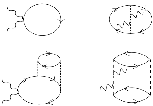
Figure 6: Some selected examples for diagrams contributing to the seagull amplitude $M_{\rm int}$ of eq.(6.6). The seagull-type vertices in the first and third diagrams come from the terms $\propto{\mbox{\boldmath${A}$}}^{2}$ in the non-interacting part of the Hamiltonian (4.14), while the vertices in the second and fourth diagrams come from the interaction part $\delta V$.

Since we have shown that the underlying Hamiltonian (4.14) is invariant with respect to local gauge transformations generated by the effective charges, the amplitude (6.6) must satisfy current conservation, in particular

$$q_{\mu}q_{\nu}T_{\rm int}^{\mu\nu}({\mbox{\boldmath${q}$}},\omega)=0\,.$$ (6.7)

Since $\omega$ and ${q}$ in this relation can be treated as independent quantities, the limit $\omega\rightarrow 0$ first followed by ${\mbox{\boldmath${q}$}}\rightarrow 0$ leads to

$$T_{\rm int}^{ij}({\mbox{\boldmath${q}$}}=0,\omega=0)=\Pi^{ij}({\mbox{\boldmath${q}$}}=0,\omega=0)+M_{\rm int}^{ij}({\mbox{\boldmath${q}$}}=0,\omega=0)=0\,.$$

(6.8)

Since $M_{\rm int}^{ij}({\mbox{\boldmath${q}$}}=0,\omega=0)=\langle 0|[[H,D^{i}],D^{j}]|0\rangle$ follows from (4.12), we immediately obtain low energy theorem (4.31). The underlying physical reason for the $\kappa-g_{\ell}$ relation can therefore be identified as the condition of current conservation for the nuclear Compton scattering amplitude.

In Appendix E we discuss further connections between the low energy Compton scattering amplitude and the orbital g-factors, making contact to the analysis in ref.[8] of photon scattering data. There we also comment on the sum rule derived a long time ago by Gerasimov [31]. It is well known that this relation seemed to indicate that the (unretarded) E1 sum rule has the same value as the integral over the total photoabsorption cross section including retardation effects and all higher order multipoles (see Appendix E). However, its validity has been questioned in a series of papers [33]-[35]. In particular, in ref. [35] it has been shown that the assumption concerning the high energy behavior of the amplitude is actually not valid due to the presence of the anomalous magnetic moment term.

7 Summary and conclusions

In this work we used the Landau-Migdal theory to discuss the orbital angular momentum g-factor of a quasiparticle and the E1 sum rule for isospin asymmetric nuclear matter. The relations obtained for the orbital g-factors are in principle exact and hold also in relativistic field theory. For the E1 sum rule, we had to restrict ourselves to a nonrelativistic framework because of the problems arising from the center of mass motion. We discussed in detail the form of the Hamiltonian which is invariant with respect to local gauge transformations generated by the effective E1 charges.

We have split the strength function into two parts, where one comes from the p-h cuts including the effects of the higher excited states via their real parts, and the other comes from cuts at higher excitation energies. We have shown generally that the former part is related to the orbital g-factors, while the latter part has no relation to them. The former part has a close relation to the collective excitations of the system, i.e., the zero sound modes in infinite systems and the giant resonances in finite nuclei. We have discussed the importance of the $\kappa-g_{\ell}$ relation, which effectively separates the observable part of the LWL sum rule, which is related to the strength function in the low energy region, from the rest. Our discussions, which do not rely on perturbation theory, can serve to put many previous investigations on the $\kappa-g_{\ell}$ relation on a theoretically firm basis.

Concerning possible extensions, we would like to remark the following points: First, the methods used here to relate $\kappa$ to $g_{\ell}$ refer to infinite nuclear matter, and it would be interesting to investigate to what extent they can be applied also to finite nuclei. Second, as we mentioned in the Introduction, very interesting attempts are now being made to extend the range of applicability of the Landau-Migdal theory [24] to give a more general description of nuclear collective vibrations. The basic idea is to generalize the definition of the quantity $A$, which appears in the equation of the vertex (2.6) etc., so as to include also more complicated configurations. It would be very interesting to see whether the results derived in this paper can be extended according to these lines.

Acknowledgements
We wish to thank Profs. Y. Horikawa, M. Ichimura, H. Sagawa, M. Schumacher, T. Suzuki (Fukui Univ.), T. Suzuki (Nihon Univ.) and K. Yazaki for helpful discussions on Giant Resonances and sum rules. This work was supported by the Grant in Aid for Scientific Research of the Japanese Ministry of Education, Culture, Sports, Science and Technology, Project No. C2-13640298.

Appendices

Appendix A Ward identities and the relativistic Landau relations for $N\neq Z$

In this Appendix we derive some relations used in sect.3, which are based on gauge and Lorentz invariance. For more detailed discussions for the case of isospin symmetric nuclear matter, we refer to refs.[26, 40].

A.1 Ward identities and currents

If $Q_{p}$ and $Q_{n}$ are the bare electric charges for protons and neutrons, the requirement of local gauge invariance leads to the Ward-Takahashi identity between the electromagnetic vertex $\Gamma_{\alpha}$ and the propagator $S_{\alpha}$ for protons ($\alpha=p$) and neutrons ($\alpha=n$):

$$q_{\mu}\Gamma_{\alpha}^{\mu}(k^{\prime},k)=Q_{\alpha}\left(S_{\alpha}^{-1}(k^{\prime})-S_{\alpha}^{-1}(k)\right)\,.$$ (A.1)

By setting $q^{0}=0$ first and then letting ${\mbox{\boldmath${q}$}}\rightarrow 0$, one obtains the Ward identity for the vertex in the “static limit” [13]:

$${\bf\Gamma}_{\alpha}^{({\rm st})}(k,k)=-Q_{\alpha}{\mbox{\boldmath${\nabla}$}}_{k}\,S_{\alpha}^{-1}(k)\,.$$ (A.2)

If the propagator has a quasiparticle pole $k_{0}=\epsilon_{\alpha}(k)$ with residue $Z_{\alpha}(k)$, we can expand $S_{\alpha}^{-1}(k)=Z_{\alpha}(k)^{-1}\left(k_{0}-\epsilon_{\alpha}(k)\right)+{\cal O}\left[\left(k_{0}-\epsilon_{\alpha}(k)\right)^{2}\right]$ to obtain the current in the static limit on the quasiparticle energy shell ($k_{0}\rightarrow\epsilon_{\alpha}(k)$) as follows:

$${\mbox{\boldmath${J}$}}_{\alpha}^{({\rm st})}(k)\equiv Z_{\alpha}(k)\,{\bf\Gamma}_{\alpha}^{({\rm st})}(k,k)=Q_{\alpha}\,{\mbox{\boldmath${\nabla}$}}_{k}\,\epsilon_{\alpha}(k)$$ (A.3)

On the Fermi surface, this gives the static current as ${\mbox{\boldmath${J}$}}_{\alpha}^{({\rm st})}(k)={\hat{\bf k}}\,Q_{\alpha}\,v_{F}(\alpha)$, where $v_{F}(\alpha)$ is the Fermi velocity for protons or neutrons.

If we take the static limit ($q_{0}\rightarrow 0$ first, then $|{\mbox{\boldmath${q}$}}|\rightarrow 0$) in eq.(LABEL:curr1) for $|{\mbox{\boldmath${k}$}}|$ on the Fermi surface, and use the form (3.3) for the p-h propagator, we can use the above form of the current in the static limit on the l.h.s. and the r.h.s. under the integral. In this kinematics the interaction $t^{(\omega)}$ depends only on the angle between the directions of ${k}$ and ${\ell}$. One then obtains the current in the “$\omega$ limit” as

$${\mbox{\boldmath${J}$}}^{(\omega)}_{\alpha}(k)={\hat{\mbox{\boldmath${k}$}}}\,Q_{\alpha}\,v_{F}(\alpha)+2\sum_{\beta=p,n}\int\frac{{\rm d}\Omega_{\ell}}{(2\pi)^{3}}\,f_{\alpha\beta}({\hat{\mbox{\boldmath${k}$}}}\cdot{\hat{\mbox{\boldmath${\ell}$}}})\,p_{F}^{2}(\beta)\,Q_{\beta}\,{\hat{\mbox{\boldmath${\ell}$}}}\,,$$ (A.4)

where $f$ is the spin independent part of $t^{(\omega)}$. The angular integrations are trivial, and if one uses the definition of the dimensionless interaction (3.4) one obtains the currents (3.5) and (3.6) for the physical charges, or (LABEL:jp1) and (LABEL:jn1) for the effective charges, where $F_{1}$ are the coefficient of the ${\ell}=1$ Legendre polynomial in the expansion of the spin independent part of the interaction ${\cal F}$.

A.2 Lorentz (Galilei) invariance for $N\neq Z$

The requirements of Lorentz invariance have been discussed in ref.[40], and are easily generalized to the case $N\neq Z$ as follows:

If we observe matter from a system ${\tilde{S}}$ which moves with velocity $-{\mbox{\boldmath${v}$}}$ relative to the system $S$ where matter is at rest, the Fermi distribution function of neutrons ($\alpha=n$) or protons ($\alpha=p$) for fixed momentum ${\ell}$ will change by an amount ${\tilde{n}}_{\ell}(\alpha)-n_{\ell}(\alpha)$, where ${\tilde{n}}$ and $n$ are the Fermi distributions in ${\tilde{S}}$ and $S$. According to Landau’s basic hypothesis [15], this corresponds to a change of the quasiparticle energy (for fixed momentum ${k}$) by an amount

$${\tilde{\epsilon}}_{k^{\prime}}(\alpha)-\epsilon_{k^{\prime}}(\alpha)=2\int\frac{{\rm d}^{3}p}{(2\pi)^{3}}\sum_{\beta=p,n}f_{\alpha\beta}(k^{\prime},\ell)\left({\tilde{n}}_{\ell}(\beta)-n_{\ell}(\beta)\right)\,,$$ (A.1)

where $f_{\alpha\beta}$ is the spin independent part of the quasiparticle interaction $t_{\alpha\beta}^{(\omega)}$, as in (A.4). On the other hand, the l.h.s. of (A.1) must agree with the result obtained from a Lorentz transformation:

$${\tilde{\epsilon}}_{k^{\prime}}(\alpha)=\gamma\left(\epsilon_{k}(\alpha)+{\mbox{\boldmath${k}$}}\cdot{\mbox{\boldmath${v}$}}\right)\,,$$ (A.2)

where ${\displaystyle\gamma=(1-{\mbox{\boldmath${v}$}}^{2})^{\frac{1}{2}}}$, and ${\mbox{\boldmath${k}$}}^{\prime}$ and ${k}$ are related by the Lorentz transformation

$${\mbox{\boldmath${k}$}}^{\prime}={\mbox{\boldmath${k}$}}+\epsilon_{k}(\alpha){\mbox{\boldmath${v}$}}\gamma-{\hat{\mbox{\boldmath${v}$}}}\left({\hat{\mbox{\boldmath${v}$}}}\cdot{\mbox{\boldmath${k}$}}\right)\left(1-\gamma\right)\,.$$ (A.3)

For the r.h.s. of (A.1), we use the fact that the Fermi distribution is Lorentz invariant:

$${\tilde{n}}_{\ell^{\prime}}(\alpha)=n_{\ell}(\alpha)$$ (A.4)

where ${\mbox{\boldmath${\ell}$}}^{\prime}$ and ${\ell}$ are related by a Lorentz transformation analogous to (A.3).

To first order in ${v}$ one easily obtains from (A.2), (A.3) and (A.4):

$${\tilde{\epsilon}}_{k^{\prime}}(\alpha)-\epsilon_{k^{\prime}}(\alpha) = {\mbox{\boldmath${k}$}}\cdot{\mbox{\boldmath${v}$}}-\epsilon_{k}(\alpha){\mbox{\boldmath${v}$}}\cdot{\mbox{\boldmath${v}$}}_{k}(\alpha)$$ (A.5)

$${\tilde{n}}_{\ell}(\alpha)-n_{\ell}(\alpha) = \epsilon_{\ell}(\alpha){\mbox{\boldmath${v}$}}\cdot{\hat{\mbox{\boldmath${\ell}$}}}\,\,\delta(|{\mbox{\boldmath${\ell}$}}|-p_{F}(\alpha))\,,$$ (A.6)

where ${\mbox{\boldmath${v}$}}_{k}(\alpha)={\mbox{\boldmath${\nabla}$}}_{k}\epsilon_{k}(\alpha)$ is the quasiparticle velocity. Inserting the relations (A.5) and (A.6) into (A.1) and setting $|{\mbox{\boldmath${k}$}}|=p_{F}(\alpha)$, we obtain

$$v_{F}(p)+\frac{v_{F}}{6}\left[\left(\frac{p_{F}(p)}{p_{F}}\right)^{2}F_{1}(pp)+\frac{\mu_{n}}{\mu_{p}}\left(\frac{p_{F}(n)}{p_{F}}\right)^{2}F_{1}(pn)\right] = \frac{p_{F}(p)}{\mu_{p}}$$

$$v_{F}(n)+\frac{v_{F}}{6}\left[\left(\frac{p_{F}(n)}{p_{F}}\right)^{2}F_{1}(nn)+\frac{\mu_{p}}{\mu_{n}}\left(\frac{p_{F}(p)}{p_{F}}\right)^{2}F_{1}(pn)\right] = \frac{p_{F}(n)}{\mu_{n}}$$

where $\mu_{\alpha}=\epsilon_{F}(\alpha)$ are the chemical potentials (Fermi energies) of protons and neutrons. These relations were used to derive eqs.(3.7), (3.8) and (4.36) in the main text.

Appendix B Local gauge invariance of the Hamiltonian (4.12)

Here we show the invariance of the Hamiltonian (4.12) under local gauge transformations up to ${\cal O}(e^{2})$. For this, we note that the arguments given below eq.(LABEL:th1) in the main text show that for any operator ${\cal B}$, which commutes with the z-component of the total isospin operator ($[T_{z},{\cal B}]=0$), the gauge transformations like (4.7) or (LABEL:th1) can be expressed by the dipole operator. That is, if $[T_{a},{\cal B}]=0$, the gauge transformation of ${\cal B}$ can be expressed as follows:

$${\cal B}\rightarrow{\rm exp}\left[-i{\mbox{\boldmath${c}$}}\cdot{\mbox{\boldmath${D}$}}\right]\,{\cal B}\,{\rm exp}\left[i{\mbox{\boldmath${c}$}}\cdot{\mbox{\boldmath${D}$}}\right]={\cal B}-ic^{i}[D^{i},{\cal B}]-\frac{1}{2}c^{i}c^{j}[D^{i},[D^{j},{\cal B}]]+\dots$$

(B.1)

We have to apply this transformation, together with

$${\mbox{\boldmath${A}$}}\rightarrow{\mbox{\boldmath${A}$}}+{\mbox{\boldmath${c}$}}$$ (B.2)

to the Hamiltonian (4.12). First, since $[T_{z},H]=0$, we can use eq.(B.1) for ${\cal B}=H$, as we have done already in (4.11) of the main text. Second, also for the single commutator term on the r.h.s. of (4.12) we have $[T_{z},[D^{i},H]]=0$, as can be seen easily from the Jacobi identity for double commutators. Third, the last term in (4.12) is already of ${\cal O}(e^{2})$, and therefore it is affected only by the gauge transformation of ${A}$, eq.(B.2). We therefore obtain for the gauge transformation of the Hamiltonian (4.12):

$${\cal H} \rightarrow {\rm exp}\left[-i{\mbox{\boldmath${c}$}}\cdot{\mbox{\boldmath${D}$}}\right]\left(H+i\left(A^{j}+c^{j}\right)[D^{j},H]\right){\rm exp}\left[i{\mbox{\boldmath${c}$}}\cdot{\mbox{\boldmath${D}$}}\right]$$ (B.3)

$$- \frac{1}{2}\left(A^{i}A^{j}+2A^{i}c^{j}+c^{i}c^{j}\right)[D^{i},[D^{j},H]]$$

Using then (B.1) for ${\cal B}=H$ and ${\cal B}=i[D^{i},H]$, it is easy to see that we simply get back the three terms on the r.h.s. of (4.12), which shows the gauge invariance of ${\cal H}$.

Appendix C Time-ordered diagrams

In this Appendix, we first explain the three points stated in sect. 5 concerning the relation between $\Pi_{A}$, which was originally defined in the language of Feynman diagrams in sect.2, and the time-ordered Bethe-Goldstone diagrams. Although the arguments presented below can be generalized by using dispersion representations for the vertex, the interaction and the self energy, we prefer to discuss representative examples in order to be definite. The arguments can be applied immediately also to other cases. We then will derive the relation (5.2).

C.1 2p-2h states induced by vertex corrections

The third diagram in Fig. 4 arises from the contribution to the quasiparticle vertex $\Gamma^{(\omega)}$ which is shown in Fig. 7. By performing the frequency integrals for the two loops, one obtains the energy denominators

$$\left[\left(k_{0}+\frac{\omega}{2}-E_{1}\right)\left(k_{0}-\frac{\omega}{2}-E_{2}\right)\right]^{-1}\,,$$ (C.1)

where the energies $E_{1}$ and $E_{2}$ are indicated in Fig.7.

Figure 7: A contribution to the vertex $\Gamma^{(\omega)}$, which is associated with the factor (C.1).

If this vertex appears in a Feynman diagram together with the p-h propagator $A$ of eq.(2.18), the effect of $A$ is to replace the energy denominator (C.1) by

$$\left[\left(\epsilon_{\lambda_{+}}-E_{1}\right)\left(\epsilon_{\lambda_{-}}-E_{2}\right)\right]^{-1}$$ (C.2)

This is the “high energy denominator” of $\Pi_{A}$. On the other hand, the high energy denominator in the time-ordered diagram (third diagram of Fig. 4) is

$$\left[\left(\omega+\epsilon_{\lambda_{-}}-E_{1}\right)\left(\epsilon_{\lambda_{-}}-E_{2}\right)\right]^{-1}$$ (C.3)

If we replace $\omega\rightarrow E^{\rm ph}\equiv\epsilon_{\lambda_{+}}-\epsilon_{\lambda_{-}}$ in (C.3), the expression agrees with (C.2). In other words, if we replace in the high energy denominator of the time-ordered graph $\omega$ by the excitation energy of the p-h pair which enters (or leaves) the vertex, we obtain the contribution of this graph to $\Pi_{A}$. This is the content of point 1. discussed in sect. 5.

C.2 2p-2h states induced by the interaction

The fifth diagram in Fig. 4 arises from the contribution to the quasiparticle interaction $T^{(\omega)}$ which is shown in Fig. 8. By performing the frequency integral for the loop, one obtains the energy denominator

$$\left[k_{0}-\ell_{0}-E\right]^{-1}\,,$$ (C.4)

where the energy $E$ is indicated in Fig. 8.

Figure 8: A contribution to the interaction $T^{(\omega)}$, which is associated with the factor (C.4).

If this interaction appears in a Feynman diagram together with two p-h propagators $A$, which correspond to the incoming and outgoing p-h pairs, the effect of $A$ (see eq.(2.18)) is to replace the energy denominator (C.1) by

$$\left[\frac{1}{2}\left(\epsilon_{\lambda_{+}}+\epsilon_{\lambda_{-}}-\epsilon_{\lambda^{\prime}_{+}}-\epsilon_{\lambda^{\prime}_{-}}\right)-E\right]^{-1}\,.$$ (C.5)

This is the “high energy denominator” of $\Pi_{A}$. On the other hand, the high energy denominator in the time-ordered diagram (fifth diagram of Fig. 4) is

$$\left[\omega+\epsilon_{\lambda_{-}}-\epsilon_{\lambda^{\prime}_{+}}-E\right]^{-1}\,.$$ (C.6)

If we replace $\omega\rightarrow\frac{1}{2}\left(E_{i}^{\rm ph}+E_{f}^{\rm ph}\right)\equiv\frac{1}{2}\left(\epsilon_{\lambda_{+}}-\epsilon_{\lambda_{-}}+\epsilon_{\lambda^{\prime}_{+}}-\epsilon_{\lambda^{\prime}_{-}}\right)$ in (C.6), the expression agrees with (C.5). In other words, if we replace in the high energy denominator of the time-ordered graph $\omega$ by the average of the excitation energies of the p-h pair which enters and leaves the interaction, we obtain the contribution of this graph to $\Pi_{A}$. This is the content of point 2. discussed in sect. 5.

C.3 2p-2h states induced by the self energy

The p-h propagator $A$ defined in sect.2 includes by definition the effects of the self energies on the quasiparticle energies and the residues. For example, if we denote by $\gamma$ the non-interacting electromagnetic vertex, the contribution $\left(i\gamma A\gamma\right)$ to $\Pi_{A}$ in eq.(2.10) includes the following factor which is associated with the diagram shown in Fig. 9a:

$$\frac{\Sigma(E_{\lambda_{+}})}{\left(\omega-E_{\lambda_{+}}+E_{\lambda_{-}}\right)^{2}}+\frac{\partial\Sigma/\partial k_{0}(E_{\lambda_{+}})}{\omega-E_{\lambda_{+}}+E_{\lambda_{-}}}\,.$$ (C.7)

Here the energies $E_{\lambda}$ do not include the effect of the dispersive self energy, which is shown in Fig. 9b. After performing the frequency integrals for the two loops in the Feynman diagram for $\Sigma$, one obtains the energy denominator

$$\left(k_{0}+\frac{\omega}{2}-E\right)^{-1}\,,$$ (C.8)

where the energy $E$ is indicated in Fig. 9b.

Figure 9: (a) A contribution of dispersive self energies to the polarization. (b) A dispersive self energy part, which is associated with the factor (C.8).

Using this in eq.(C.7), we see that the high energy denominators in $\Pi_{A}$ have the form

$$\left[\left(\omega-E_{\lambda_{+}}+E_{\lambda_{-}}\right)^{2}\left(E_{\lambda_{+}}-E\right)\right]^{-1}-\left[\left(\omega-E_{\lambda_{+}}+E_{\lambda_{-}}\right)\left(E_{\lambda_{+}}-E\right)^{2}\right]^{-1}\,.$$

(C.9)

On the other hand, the high energy denominators of the time-order diagram for the polarization are

$$\left[\left(\omega-E_{\lambda_{+}}+E_{\lambda_{-}}\right)^{2}\left(\omega+E_{\lambda_{-}}-E\right)\right]^{-1}$$ (C.10)

Expanding the high energy denominator (second factor in (C.10)) around $\omega=E_{\lambda_{+}}-E_{\lambda_{-}}$ and taking only the first two terms of this expansion, we obtain an expression which agrees with (C.9). In other words, if we replace the high energy denominator of the time-ordered graph by its first two terms of an expansion around the excitation energy of the p-h pair under consideration, we obtain the contribution of this graph to $\Pi_{A}$. This is the content of point 3. discussed in sect. 5.

C.4 Proof of relation (5.1)

For each time-order graph which contributes to the polarization, there is another one which is obtained from the original graph by crossing the photon lines. That is, each graph $\Pi^{(i)}$, which is characterized by a particular topology of the internal propagators and two-body interactions, can be split into two parts, $\Pi^{(i)}=\Pi^{(i)}_{+}+\Pi^{(i)}_{-}$, where $\Pi^{(i)}_{+}$ does not involve crossed photons (“forward term”), and $\Pi^{(i)}_{-}$ involves crossed photons (“backward term”). By definition, the intermediate states in $\Pi^{(i)}_{+}$ have either no photons (energy denominators of the form $\left(\omega-E_{n}+i\epsilon\right)^{-1}$), or one photon (energy denominators are independent of $\omega$). On the other hand, the intermediate states in $\Pi^{(i)}_{-}$ have either two photons (energy denominators of the form $\left(\omega+E_{n}-i\epsilon\right)^{-1}$), or one photon (energy denominators are independent of $\omega$). It follows that $\Pi^{(i)}_{+}(\omega)$ is analytic in the upper $\omega$ plane [39], and has a non-vanishing imaginary part only for real positive $\omega$. From these properties it follows that $\Pi^{(i)}_{+}(\omega)$ satisfies a dispersion relation

$$\Pi^{(i)}_{+}(\omega)=\frac{-1}{\pi}\int_{0}^{\infty}\frac{{\rm d}\omega^{\prime}}{\omega-\omega^{\prime}+i\epsilon}\,\,{\rm Im}\,\,\Pi^{(i)}_{+}(\omega^{\prime})\,.$$ (C.11)

Since $\Pi^{(i)}_{+}(\omega)$ and $\Pi^{(i)}_{-}(\omega)$ differ only by the external photon lines, they give the same contribution at $\omega=0$, that is, $\Pi^{(i)}_{+}(\omega=0)=\Pi^{(i)}_{-}(\omega=0)$. We therefore obtain from eq.(C.11) in the limit $\omega=0$

$$\int_{0}^{\infty}\frac{{\rm d}\omega}{\omega}\,\,{\rm Im}\,\Pi^{(i)}(\omega)=\int_{0}^{\infty}\frac{{\rm d}\omega}{\omega}\,\,{\rm Im}\,\Pi^{(i)}_{+}(\omega)$$ (C.12)

$$=\pi\,\Pi^{(i)}_{+}(\omega=0)=\frac{\pi}{2}\,\Pi^{(i)}(\omega=0)\,,$$

which is the content of eq.(5.1).

Appendix D Connection between $\Pi_{A}$ and the collective excitations

In this Appendix we derive the expression for the polarization $\Pi_{A}$ in terms of the solutions to the Landau equation, referring for simplicity to symmetric nuclear matter (N=Z) and low energy and momentum transfer, where $\Pi_{A}$ of eq.(2.21) depends only on the ratio $s=\omega/(|{\mbox{\boldmath${q}$}}|v_{F})$. For the case N=Z, the effective charges (4.18) become $\pm\frac{1}{2}e_{p}$ for protons and neutrons, and therefore the currents in the polarization (2.21) are the isovector (IV) currents.

If we approximate the p-h propagator in (2.21) by (3.3), the quantity

$${\mbox{\boldmath${\phi}$}}({\mbox{\boldmath${k}$}},s) \equiv \frac{{\mbox{\boldmath${q}$}}\cdot{\hat{\mbox{\boldmath${k}$}}}\,\delta(k-p_{F})}{\omega-{\mbox{\boldmath${q}$}}\cdot{\mbox{\boldmath${v}$}}_{k}+i\gamma}\,{\mbox{\boldmath${j}$}}_{\rm IV}(k_{+},k_{-})\equiv\delta(|{\mbox{\boldmath${k}$}}|-p_{F})\,{\mbox{\boldmath${\phi}$}}({\hat{\mbox{\boldmath${k}$}}},s)$$

satisfies the equation

$$\left(s-\cos\Theta_{k}\right){\mbox{\boldmath${\phi}$}}({\hat{\mbox{\boldmath${k}$}}},s)=\frac{\cos\Theta_{k}}{v_{F}}\,{\mbox{\boldmath${j}$}}_{\rm IV}^{(\omega)}({\hat{\mbox{\boldmath${k}$}}})+\frac{\cos\Theta_{k}}{4\pi}\int{\rm d}\Omega_{\ell}\,F^{\prime}({\hat{\mbox{\boldmath${k}$}}}\cdot{\hat{\mbox{\boldmath${\ell}$}}})\,{\mbox{\boldmath${\phi}$}}({\hat{\mbox{\boldmath${\ell}$}}},s)\,,$$

(D.2)

where $\cos\Theta_{k}\equiv{\hat{\mbox{\boldmath${q}$}}}\cdot{\hat{\mbox{\boldmath${k}$}}}$, $F^{\prime}({\hat{\mbox{\boldmath${k}$}}}\cdot{\hat{\mbox{\boldmath${\ell}$}}})$ is the spin independent part $\propto({\mbox{\boldmath${\tau}$}}_{1}\cdot{\mbox{\boldmath${\tau}$}}_{2})$ of the dimensionless Landau-Migdal interaction (3.4), and ${\mbox{\boldmath${j}$}}^{(\omega)}_{\rm IV}({\hat{\mbox{\boldmath${k}$}}})$ is the isovector part of the quasiparticle current in the $\omega$-limit at the Fermi surface, i.e., from eqs. (3.7), (3.8):

$${\mbox{\boldmath${j}$}}^{(\omega)}_{\rm IV}({\hat{\mbox{\boldmath${k}$}}})\equiv{\hat{\mbox{\boldmath${k}$}}}\,j^{(\omega)}_{\rm IV}={\hat{\mbox{\boldmath${k}$}}}\,\frac{1}{2}\,\left(\frac{p_{F}}{M}-\frac{v_{F}}{3}\left(F_{1}-F_{1}^{\prime}\right)\right).$$ (D.3)

For small $|{\mbox{\boldmath${q}$}}|$ it is sufficient to seek the solution to (D.2) in the form ${\mbox{\boldmath${\phi}$}}({\hat{\mbox{\boldmath${k}$}}},s)\equiv{\hat{\mbox{\boldmath${k}$}}}\,\phi({\hat{\mbox{\boldmath${k}$}}},s)$, where the scalar function $\phi({\hat{\mbox{\boldmath${k}$}}},s)$ satisfies an equation similar to (D.2), but with the interaction retarded by one unit of angular momentum: ${\cal F}({\hat{\mbox{\boldmath${k}$}}}\cdot{\hat{\mbox{\boldmath${\ell}$}}})\rightarrow{\cal F}({\hat{\mbox{\boldmath${k}$}}}\cdot{\hat{\mbox{\boldmath${\ell}$}}})\,{\hat{\mbox{\boldmath${k}$}}}\cdot{\hat{\mbox{\boldmath${\ell}$}}}$. We can write the equation for $\phi({\hat{\mbox{\boldmath${k}$}}},s)$ in the form

$$\int{\rm d}\Omega_{\ell}\,K({\hat{\mbox{\boldmath${k}$}}},{\hat{\mbox{\boldmath${\ell}$}}})\,\phi({\hat{\mbox{\boldmath${\ell}$}}},s)+\frac{\cos\Theta_{k}}{v_{F}}j_{\rm IV}^{(\omega)}=s\,\phi({\hat{\mbox{\boldmath${k}$}}},s)$$ (D.4)

with the kernel

$$K({\hat{\mbox{\boldmath${k}$}}},{\hat{\mbox{\boldmath${\ell}$}}})\equiv\cos\Theta_{k}\,\delta(\Omega_{k}-\Omega_{\ell})+\frac{\cos\Theta_{k}}{4\pi}F^{\prime}({\hat{\mbox{\boldmath${k}$}}}\cdot{\hat{\mbox{\boldmath${\ell}$}}})\,{\hat{\mbox{\boldmath${k}$}}}\cdot{\hat{\mbox{\boldmath${\ell}$}}}.$$ (D.5)

One can express the solution to the inhomogeneous equation (D.4) by the solutions to the homogenoues equations

$$\int{\rm d}\Omega_{\ell}\,K({\hat{\mbox{\boldmath${k}$}}},{\hat{\mbox{\boldmath${\ell}$}}})\,\Phi({\hat{\mbox{\boldmath${\ell}$}}},s) = s\,\Phi({\hat{\mbox{\boldmath${k}$}}},s)$$ (D.6)

$$\int{\rm d}\Omega_{k}\,\overline{\Phi}({\hat{\mbox{\boldmath${k}$}}},s)\,K({\hat{\mbox{\boldmath${k}$}}},{\hat{\mbox{\boldmath${\ell}$}}}) = s\,{\overline{\Phi}}({\hat{\mbox{\boldmath${\ell}$}}},s)\,,$$ (D.7)

where we must distinguish between the right and left eigenfunctions because of the nonhermiticity of the kernel $K$. The left eigenfunction is related to the ordinary h.c. of $\Phi$ by ${\displaystyle\overline{\Phi}({\hat{\mbox{\boldmath${k}$}}},s)=\Phi^{\dagger}({\hat{\mbox{\boldmath${k}$}}},s)\frac{N_{s}}{\cos\Theta_{k}}}$, where $N_{s}$ is chosen to satisfy the normalization (D.9).

For $|s|<1$ there exist “free” solutions to eq.(D.6) and (D.7), namely ${\displaystyle\Phi({\hat{\mbox{\boldmath${k}$}}},s)={\overline{\Phi}}({\hat{\mbox{\boldmath${k}$}}},s)=\frac{1}{\sqrt{2\pi}}\delta(s-\cos\Theta_{k})}$, and in this case the homogeneous equations can be solved iteratively for any value $|s|<1$, i.e., there is a continuum of solutions. For $|s|>1$, on the other hand, no free solutions exist, and the eigenvalue $s$ becomes discrete. These are the zero sound solutions, which have been investigated in detail in many works [28, 41, 16].

We can choose the right and left eigenfunctions so as to form a complete orthonormal set:

$$\int{\rm d}\Omega_{k}\,{\overline{\Phi}}({\hat{\mbox{\boldmath${k}$}}},s^{\prime})\,\Phi({\hat{\mbox{\boldmath${k}$}}},s)=\delta_{s^{\prime},s}$$ (D.9)

$${\sum}_{s}\Phi({\hat{\mbox{\boldmath${k}$}}},s)\,{\overline{\Phi}}({\hat{\mbox{\boldmath${\ell}$}}},s)=\delta\left(\Omega_{k}-\Omega_{\ell}\right)\,,$$

where $\delta_{s^{\prime},s}$ stands for a delta function in the case of continous eigenvalues, and the Kronecker delta symbol in the case of discrete ones. The symbol $\sum_{s}$ refers to an integral over continuous eigenvalues, and a sum over discrete ones. The solution to the inhomogeneous equation (D.4) can then be expressed as follows:

$$\phi({\hat{\mbox{\boldmath${k}$}}},s)=\frac{j_{\rm IV}^{(\omega)}}{v_{F}}\,{\sum}_{s^{\prime}}\,\int{\rm d}\Omega_{\ell}\,\frac{\Phi({\hat{\mbox{\boldmath${k}$}}},s^{\prime}){\overline{\Phi}}({\hat{\mbox{\boldmath${\ell}$}}},s^{\prime})}{s-s^{\prime}+i\gamma}\,\cos\Theta_{\ell}\,,$$ (D.10)

where $\cos\Theta_{\ell}={\hat{\mbox{\boldmath${q}$}}}\cdot{\hat{\mbox{\boldmath${\ell}$}}}$. Returning to the correlation function (2.21), we obtain in the limit of low $(\omega,{\mbox{\boldmath${q}$}})$ the form $\Pi_{A}^{ij}(\omega,{\mbox{\boldmath${q}$}})=\delta^{ij}\Pi_{A}(\omega,{\mbox{\boldmath${q}$}})$, where $\Pi_{A}$ is given by

$$\Pi_{A}(\omega,{\mbox{\boldmath${q}$}}) = -\frac{Vp_{F}^{2}}{6\pi^{3}}\,j_{\rm IV}^{(\omega)}\,\int{\rm d}\Omega_{k}\,\phi({\hat{\mbox{\boldmath${k}$}}},s)=-\frac{A}{4p_{F}v_{F}}\,\left(j_{\rm IV}^{(\omega)}\right)^{2}\,\frac{{\sum}_{s^{\prime}}\,A_{s^{\prime}}\,B_{s^{\prime}}}{s-s^{\prime}+i\gamma}\,,$$

where

$$A_{s^{\prime}} = \int{\rm d}\Omega_{k}\,\Phi({\hat{\mbox{\boldmath${k}$}}},s^{\prime})$$

$$B_{s^{\prime}} = \int{\rm d}\Omega_{k}\,{\overline{\Phi}}({\hat{\mbox{\boldmath${k}$}}},s^{\prime})\,\cos\Theta_{k}\,=A_{s^{\prime}}^{*}\,N_{s^{\prime}}\,.$$ (D.12)

From the homogeneous equations (D.6) and (D.7) it is easy to see that by reversing the direction of the momentum one obtains a solution with the opposite sign of the eigenvalue: $\Phi(-{\hat{\mbox{\boldmath${k}$}}},s)=\Phi({\hat{\mbox{\boldmath${k}$}}},-s)$ and ${\overline{\Phi}}(-{\hat{\mbox{\boldmath${k}$}}},s)={\overline{\Phi}}({\hat{\mbox{\boldmath${k}$}}},-s)$. One can therefore restrict the summation over the eigenvalues in (LABEL:re1) to positive ones and write

$$\Pi_{A}(\omega,{\mbox{\boldmath${q}$}})=-\frac{A}{4p_{F}v_{F}}\,\left(j_{\rm IV}^{(\omega)}\right)^{2}\,{\sum}_{s^{\prime}}\,|A_{s^{\prime}}|^{2}\,N_{s^{\prime}}\,\left(\frac{1}{s-s^{\prime}+i\gamma}-\frac{1}{s+s^{\prime}-i\gamma}\right)\,.$$

(D.13)

Appendix E Some relations for the Compton scattering amplitude

In this Appendix we discuss relations between the low energy Compton scattering amplitude and the orbital g-factors (or the enhancement factor $1+\kappa_{A}$), and make contact to the sum rule derived a long time ago by Gerasimov [31].

E.1 Relations for the low energy scattering amplitudes

If we add the Thomson amplitude

$$M^{ij}_{\rm Th}=\delta^{ij}\,\,\frac{-Z^{2}\,e_{p}^{2}}{MA}$$ (E.1)

to the intrinsic part (6.6), we get the total photon scattering amplitude

$$T^{ij}({\mbox{\boldmath${q}$}},\omega)=\Pi^{ij}({\mbox{\boldmath${q}$}},\omega)+M^{ij}({\mbox{\boldmath${q}$}},\omega)$$ (E.2)

with $M\equiv M_{\rm int}+M_{\rm Th}$. Similar to the correlation function $\Pi$, we can split also the seagull amplitude into two parts as $M=M_{A}+M_{B}$. (Examples for $M_{A}$ are shown by the first three diagrams in Fig. 6, while the fourth diagram contributes to $M_{B}$.)

According to eqs.(4.37), (3.12), and (6.8), the “A-parts” of the scattering amplitude (E.2) can be expressed in terms of the orbital g-factors, or in terms of $\kappa_{A}$, as follows:

$$\Pi^{ij}_{A}({\mbox{\boldmath${q}$}}=0,\omega=0) = \delta^{ij}\,e_{p}^{2}\,\frac{NZ}{AM}\left(g_{\ell}(p)-g_{\ell}(n)\right)=e_{p}^{2}\,\frac{NZ}{AM}\left(1+\kappa_{A}\right)$$

$$M^{ij}_{A}({\mbox{\boldmath${q}$}}=0,\omega=0) = -\Pi_{A}^{ij}({\mbox{\boldmath${q}$}}=0,\omega=0)-\frac{Z^{2}\,e_{p}^{2}}{MA}$$ (E.4)

$$= -\frac{Z\,e_{p}^{2}}{M}g_{\ell}(p)=-\frac{Z\,e_{p}^{2}}{M}\left(1+\frac{N}{A}\kappa_{A}\right).$$

These relations between the low energy nuclear Compton scattering amplitudes and the E1 enhancement factor have been used extensively in the analysis of experimental data [8]. One should keep in mind, however, that they are valid only for the “A-parts”. The “B-parts” of $\Pi$ and $M$, which cancel each other in the low energy limit, have no relations to the orbital g-factors.

E.2 Relation to Gerasimov’s sum rule

In sect. 4 we made use of a spectral representation of the correlation function for fixed ${q}$, see eq.(4.26). Although for a real photon one has $|{\mbox{\boldmath${q}$}}|=\omega$, in the energy region where $\omega\,R<<1$ one can approximate $|{\mbox{\boldmath${q}$}}|\simeq 0$, leaving $\omega$ finite. This leads to the unretarded E1 sum rule (4.23), (4.24). On the other hand, there exists a subtracted dispersion relation for the full forward scattering amplitude $T(\omega)\equiv T_{ij}({\mbox{\boldmath${q}$}},\omega)\,e_{i}\,e_{j}$ for a physical photon ($|{\mbox{\boldmath${q}$}}|=\omega$) [32]:

$${\rm Re}\,T(\omega)-T(\omega=0)=-\frac{\omega^{2}}{2\pi^{2}}P\int_{0}^{\infty}dE\,\frac{1}{\omega^{2}-E^{2}}\,\sigma_{\rm tot}(E).$$ (E.5)

This dispersion relation is often used to extract the total photoabsorption cross section $\sigma_{\rm tot}$ from the measured elastic cross section [10, 11, 8].

According to eq.(E.2), the amplitude $T$ consists of the “resonance amplitude” $\Pi(\omega)\equiv\Pi_{ij}(\omega)\,e_{i}\,e_{j}$ and the “seagull amplitude” $M(\omega)\equiv M_{ij}(\omega)\,e_{i}\,e_{j}$. In the energy region beyond the GDR and below the pion production threshold ($\omega_{\rm GDR}<<\omega<<\omega_{\pi}$), the energy dependence of the seagull amplitude $M$ (fig.6) is weak: $M(\omega)\simeq M(\omega=0)$. Therefore one can replace $T\rightarrow\Pi$ on the l.h.s. of (E.5) to get the relation

$${\rm Re}\,\Pi(\omega)-\Pi(\omega=0)=-\frac{\omega^{2}}{2\pi^{2}}P\int_{0}^{\infty}dE\,\frac{1}{\omega^{2}-E^{2}}\,\sigma_{\rm tot}(E)\,,$$ (E.6)

which is valid for $\omega_{\rm GDR}<<\omega<<\omega_{\pi}$. If one makes the further assumption that in this energy region ($\omega>>\omega_{GDR}$) the resonance amplitude $\Pi(\omega)$ is already small because of large energy denominators, one might use (E.6) formally also for $\omega\rightarrow\infty$ to obtain

$$\Pi(\omega=0)\stackrel{{\scriptstyle?}}{{=}}\frac{1}{2\pi^{2}}P\int_{0}^{\infty}dE\,\sigma_{\rm tot}(E)\,,$$ (E.7)

and comparison with the exact relation (4.28) would lead to

$$\int_{0}^{\infty}dE\,S(E)\stackrel{{\scriptstyle?}}{{=}}\int_{0}^{\infty}dE\,\sigma_{\rm tot}(E).$$ (E.8)

This conjecture due to Gerasimov [31] has often been interpreted as the “cancellation between retardation effects and higher order multipoles” [3],[33]-[35], since the l.h.s. of (E.8) involves only the unretarded E1 multipole, while the r.h.s. involves the total cross section. It has, however, been shown explicitly in ref. [35] that the assumption (E.7) on the high energy behaviour of the resonance amplitude is not valid due to the contribution of the anomalous magnetic moment term to the dispersion integral. Therefore it was pointed out that eqs. (E.7) and (E.8) are actually not valid.

References

- [1] J.S. Levinger and H.A. Bethe, Phys. Rev. 78 (1950) 115.
- [2] H. Miyazawa, Prog. Theor. Phys. 6 (1951) 801.
- [3] J.-I. Fujita and M. Ichimura, Mesons in Nuclei, Vol. II (D.H. Wilkinson and M. Rho, eds.), North-Holland, Amsterdam 1979, p. 625.
- [4] T. Yamazaki, Mesons in Nuclei, Vol. II (D.H. Wilkinson and M. Rho, eds.), North-Holland, Amsterdam 1979, p.651.
- [5] J.-I. Fujita and M. Hirata, Phys. Lett. 37 B (1971) 237.
- [6] A. Arima, G.E. Brown, H. Hyuga and M. Ichimura, Nucl. Phys. A 205 (1973) 27.
- [7] J.-I. Fujita, S. Ishida and M. Hirata, Progr. Theor. Phys. Suppl. 60 (1976) 73.
-
[8]
M. Schumacher, A.I. Milstein, H. Falkenberg, K. Fuhrberg, T. Glebe,
D. Häger and M. Hütt, Nucl. Phys. A 576 (1994) 603;
M. Schumacher, Nucl. Phys. A 629 (1998) 334c;
M. Hütt, A.I. L’vov, A.I. Milstein and M. Schumacher, Phys. Rep. 323 (2000) 457. - [9] B.L. Berman and S.C. Fultz, Rev. Mod. Phys. 47 (1975) 713.
- [10] R. Nolte, A. Baumann, K.W. Rose and M. Schumacher, Phys. Lett. B 173 (1986) 388.
- [11] D.S. Dale, A.M. Nathan, F.J. Federspiel, S.D. Hoblit, J. Hughes and D. Wells, Phys. Lett. B 214 (1988) 329.
- [12] A.B. Migdal, A.A. Lushnikov and D.F. Zaretsky, Nucl. Phys. 66 (1965) 193.
- [13] A.B. Migdal, Theory of finite Fermi systems and applications to atomic nuclei, Wiley, New York, 1967.
- [14] M. Ichimura, Nucl. Phys. A 522 (1991) 201c.
-
[15]
L.D. Landau, JETP 3 (1957) 920; 5 (1957) 101; 8 (1959) 70;
For a review, see: G. Baym and Ch. Pethick, The Physics of Liquid and Solid Helium, Part II (Wiley, 1978), p. 1. - [16] P. Nozieres, Theory of Interacting Fermi Systems (W.A. Benjamin, 1964).
- [17] E. Lipparini and S. Stringari, Phys. Rep. 175 (1989) 103.
- [18] J. Speth and J. Wambach, in Electric and magnetic giant resonances (ed. J. Speth), World Scientific (1991) 1.
- [19] See the recent proceedings on conferences on Giant Resonances: Nucl. Phys. A 569 (1994), A 599 (1996), A 649 (1999), A 687 (2001).
- [20] M. Harakeh and A. can der Woude, Giant Resonances (Clarendon Press, Oxford, 2001).
- [21] T. Aumann, P.F. Bortignon and H. Emling, Annu. Rev. Nucl. Part. Sci. 48 (1998) 351.
-
[22]
T. Aumann et al, Nucl. Phys. A 649 (1999);
H. Sagawa and T. Suzuki, Phys. Rev. C 59 (1999) 3116. -
[23]
S. Kamerdzhiev, J. Speth, G. Tertychny and V. Tselyaev, Nucl. Phys. A 555 (1993) 90;
S. Kamerdzhiev, J. Speth and G. Tertychny, Nucl. Phys. A 624 (1997) 328. - [24] S. Kamerdzhiev, J. Speth and G. Tertychny, Extended Theory of Finite Fermi Systems: Collective Vibrations in Closed Shell Nuclei, nucl-th/0311058.
- [25] J.M. Eisenberg and W. Greiner, Nuclear Theory, Vol. 2 (North-Holland, 1970), chapt. 5.
- [26] W. Bentz, A. Arima, H. Hyuga, K. Shimizu and K. Yazaki, Nucl. Phys. A 436 (1985) 593.
- [27] A. Arima, K. Shimizu, W. Bentz and H. Hyuga, Adv. Nucl. Phys. 18 (1987) 1.
- [28] K. Tanaka, W. Bentz and A. Arima, Nucl. Phys. A 555 (1993) 151.
- [29] G.E. Brown and M. Rho, Nucl. Phys. A 338 (1980) 269.
- [30] M. Ichimura, H. Hyuga and G.E. Brown, Nucl. Phys. A 196 (1972) 17.
- [31] S.B. Gerasimov, Phys. Lett. 13 (1964) 240.
- [32] M. Gell-Mann, M.L. Goldberger and W.E. Thirring, Phys. Rev. 95 (1954) 1612.
- [33] T. Matsuura and K. Yazaki, Phys. Lett. B 46 (1973) 17.
- [34] J.L. Friar and S. Fallieros, Phys. Rev. C 11 (1975) 274.
- [35] H. Arenhövel and D. Drechsel, Phys. Rev. C 20 (1979) 1965.
- [36] K. Shimizu, M. Ichimura and A. Arima, Nucl. Phys. A 226 (1974) 282.
- [37] R. Silbar, C. Wentz and H. Überall, Nucl. Phys. A 107 (1968) 655.
-
[38]
P. Christillin and M. Rosa-Clot, Phys. Lett. B 51 (1974) 125;
P. Christillin, J. Phys. G 12 (1986) 837. - [39] K. Takayanagi, Nucl. Phys. A 510 (1990) 162.
- [40] G. Baym and S.A. Chin, Nucl. Phys. A 262 (1976) 527.
- [41] T. Yukawa and G. Holzwarth, Nucl. Phys. A 364 (1981) 29.