Sensitivity of exclusive proton knockout spin observables to different Lorentz invariant representations of the NN interaction

Abstract

Within the framework of the relativistic plane wave impulse approximation, we study the observable consequences of employing a complete Lorentz invariant representation of the NN scattering matrix in terms of 44 independent amplitudes, as opposed to the previously-employed, but ambiguous, five-term Lorentz invariant parametrization of the NN scattering matrix, for the prediction of complete sets of exclusive ($\vec{p},2\vec{p}\,$) polarization transfer observables. Two kinematic conditions are considered, namely proton knockout from the $3s_{1/2}$ state of ²⁰⁸Pb at an incident energy of 202 MeV for coplanar scattering angles ($28.0^{\circ},-54.6^{\circ}$), as well as an incident energy of 392 MeV for the angle pair ($32.5^{\circ},-80.0^{\circ}$). The results indicate that certain spin observables are ideal for discriminating between the two representations.

I Introduction

The representation of the nucleon-nucleon (NN) scattering matrix, within the context of an appropriate dynamical framework is crucial for the description of nuclear reactions and nuclear structure.

Recently, we demonstrated that a model based on the relativistic distorted wave impulse approximation (DWIA) provides an almost perfect description of exclusive ($\vec{p},2p$) analyzing power data, whereas corresponding nonrelativistic Schrödinger-equation-based predictions completely fail Ne02 ; Hi03a ; Hi03b . For both dynamical models, however, the comparison of theoretical predictions to unpolarized cross section data yields similar spectroscopic factors which are also in good agreement with those extracted from ($e,e^{\prime}p$) studies. The above results highlight the important role that spin observables (such as the analyzing power) play, as opposed to unpolarized cross sections, in effectively discriminating between different dynamical effects and, at the same time, also pointing to the Dirac equation as the preferred equation of motion.

However, before claiming the latter statement with absolute certainty, it is necessary to subject our relativistic DWIA models to additional tests, such as comparing model predictions to additional spin observable data, other than the commonly measured analyzing power. In particular, it is important to eliminate obvious ambiguities associated with the choice of representation for the NN scattering matrix. Essentially, the problem is related to the direct application of the free on-shell NN scattering matrix for the description of nucleons scattering from nuclei: the external nucleons partaking in free on-shell NN scattering are represented by free positive-energy Dirac spinors, whereas for scattering from nuclei the scattering wave functions are linear combinations of both positive and negative- energy Dirac spinors [see Sec. (V)]. To date, all applications of Dirac relativity to describe exclusive ($p,2p$) reactions have adopted the so-called IA1 parametrization, whereby the free NN scattering matrix is parametrized in terms of five Lorentz (scalar, pseudoscalar, vector, axial-vector, and tensor) invariants which are consistent with parity and time-reversal invariance as well as charge symmetry. These invariant amplitudes are obtained by fitting to free NN scattering data. There are, however, an infinite number of five-term representations with the same on-shell matrix elements for free NN scattering, and which also respect the above symmetries Go57 ; Br76 . Hence, free on-shell NN scattering data cannot distinguish between different five-term representations. However, for applications to nuclear reactions, different five-term representations result in drastically different observables, thereby clouding physical interpretation of the data. In Refs. Hi94 ; Hi95 ; Hi98 we demonstrated the limitations of the IA1 representation for applications to inclusive quasielastic proton-nucleus scattering: for example, one type of five-term representation describes ($\vec{p},\vec{p}\,^{\prime}$) data, whereas a different representation is required for ($\vec{p},\vec{n}$) scattering.

The ambiguities associated with the IA1 representation can be eliminated by employing the more appropriate, but more complicated, IA2 representation developed by Tjon and Wallace Tj85a ; Tj85b ; Tj87a ; Tj87b , whereby the NN scattering matrix is expanded in terms of a complete set of 44 independent invariant amplitudes consistent with the above-mentioned symmetries. It follows therefore that IA1 neglects 39 additional amplitudes that should appear on the grounds of very general symmetry principles. The aim of this paper is to apply the IA2 representation, for the first time, to exclusive proton knockout reactions and to compare results to corresponding IA1 predictions of complete sets of spin observables.

We have already studied the observable consequences of employing the IA2, rather than the IA1 representation, for describing inclusive quasielastic proton-nucleus scattering Va99 ; Va00 . The aim of the latter paper was to identify spin observables which are sensitive enough to extract information regarding the modification of the properties of the strong nuclear force by nuclear matter. In particular, we demonstrated that the IA1 representation severely overestimates the importance of nuclear medium modifications on the NN interaction, whereas application of the IA2 representation suggests that quasielastic spin observables are insensitive to these effects. This emphasizes the critical role played by the representation of the NN scattering matrix in giving a correct interpretation of the results.

Although we have already demonstrated that a quantitative description of ($\vec{p},2\vec{p}\,$) spin observable data requires the inclusion of nuclear medium effects on the scattering wave functions Hi03a , in this paper we consider a relativistic plane wave approximation, thus neglecting the role of distorting optical potentials on the scattering wave functions. This simplification will allow us to uniquely focus on the effect of the different representations employed for $\hat{F}$. Two kinematic conditions are considered, namely proton knockout from the $3s_{1/2}$ state of ²⁰⁸Pb at an incident energy of 202 MeV for coplanar scattering angles $(\theta_{a^{\prime}},\theta_{b})\,=\,(28.0^{\circ},-54.6^{\circ})$, as well as an incident energy of 392 MeV for coplanar scattering angles $(\theta_{a^{\prime}},\theta_{b})\,=\,(32.5^{\circ},-80.0^{\circ})$. The reaction kinematics at 202 MeV are chosen to correspond to recent measurements by Neveling et al. Ne02 at iThemba Laboratory for Accelerator Based Sciences (Faure, South Africa), and the kinematics at 392 MeV correspond to present and future experimental programs at the Research Center for Nuclear Physics in Osaka, Japan No03 . In addition, the above kinematics are also chosen so as to minimize complications associated with the inclusion of recoil corrections in the Dirac equation Co93a ; Ma93a , while still maintaining the validity of the impulse approximation.

In Sec. (II), we present the formalism for the relativistic plane wave impulse approximation. Thereafter, in Sec. (III), we derive expressions for the relativistic scattering matrix element based on both IA1 and IA2 representations of the NN interaction. The expressions for calculating complete sets of spin observables are presented in Sec. (IV). Results are given in Sec. (V), and we summarize and draw conclusions in Sec. (VI).

II Relativistic Plane Wave Impulse Approximation

Consider an exclusive $(p,2p)$ reaction, written as $A(a,a^{\prime}b)C$ for notational purposes and depicted schematically in Fig. (1), whereby an incident proton $a$ knocks out a bound proton $b$ from a specific orbital in the target nucleus $A$, resulting in three particles in the final state, namely the recoil residual nucleus $C$ and two outgoing protons, $a^{\prime}$ and $b$, which are detected in coincidence at coplanar laboratory scattering angles (on opposite sides of the incident beam), $\theta_{a^{\prime}}$ and $\theta_{b}$, respectively. All kinematic quantities are completely determined by specifying the rest masses, $m_{i}$, of particles, where $i$ = ($a$,$A$, $a^{\prime}$, $b$, $C$), the laboratory kinetic energy $\mbox{T}_{a}$ of incident particle $a$, the laboratory kinetic energy $\mbox{T}_{a^{\prime}}$ of scattered particle $a^{\prime}$, the laboratory scattering angles $\theta_{a^{\prime}}$ and $\theta_{b^{\prime}}$, and also the binding energy of the proton that is to be knocked out of the target nucleus $A$. In this paper we employ the conventions of Bjorken and Drell Bj64 and, unless otherwise stated, all kinematic quantities are expressed in natural units (i.e., $\hbar=c=1$).

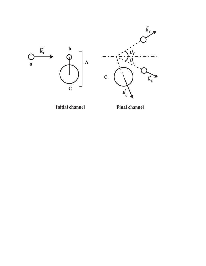
Figure 1: Schematic representation for the coplanar $(p,2p)$ reaction of interest.

For a zero range approximation to the NN interaction, the relativistic transition matrix element associated with Fig. (1) is given by Hi03a ; Hi03b :

$$T_{LJM_{J}}(s_{a},s_{a^{\prime}},s_{b}) = \int d^{3}\vec{x}\left[\bar{\psi}^{(-)}(\vec{x},\vec{k}_{a^{\prime}},s_{a^{\prime}}\,)\otimes\bar{\psi}^{(-)}(\vec{x},\vec{k}_{b},s_{b})\right]\hat{F}\left[\psi^{(+)}(\vec{x},\vec{k}_{a},s_{a})\otimes\phi_{LJM_{J}}(\vec{x})\right]$$ (1)

where $\otimes$ denotes the Kronecker product. The four-component scattering wave functions, $\psi(\vec{x},\vec{k}_{i},s_{i})$, are solutions to the fixed-energy Dirac scattering equations: $\psi^{(+)}(\vec{x},\vec{k}_{a},s_{a})$ is the relativistic scattering wave function associated with the incident particle, $a$, with outgoing boundary conditions [indicated by the superscript $(+)$], where $\vec{k}_{a}$ is the momentum of particle $a$ in the laboratory frame, and $s_{a}$ is the spin projection thereof with respect to $\vec{k}_{a}$ as the $\hat{z}$-quantization axis; $\bar{\psi}^{(-)}(\vec{x},\vec{k}_{j},s_{j})$ is the adjoint relativistic scattering wave function for particle $j$ [ $j$ = ($a^{\prime},b$)] with incoming boundary conditions [indicated by the superscript $(-)$], where $\vec{k}_{j}$ is the momentum of particle $j$ in the laboratory frame, and $s_{j}$ is the spin projection thereof with respect to $\vec{k}_{j}$ as the $\hat{z}$-quantization axis. The boundstate proton wave function, $\phi^{B}_{LJM_{J}}(\vec{x}\,)$, labeled by single-particle quantum numbers $L$, $J$, and $M_{J}$, is given by:

$$\phi_{LJM_{J}}(\vec{x}\,) = \frac{1}{x}\,\sum_{s_{B}}\,\left(\begin{array}[]{c}u_{LJ}(x)\,\langle L,M_{J}-s_{B},\frac{1}{2},s_{B}\,|J,M_{J}\,\rangle\,Y_{L,M_{J}-s_{B}}(\hat{x})\,\chi_{s_{B}}\\ iw_{LJ}(x)\,\langle 2J-L,M_{J}-s_{B},\frac{1}{2},s_{B}\,|\,J,M_{J}\,\rangle\,Y_{2J-L,M_{J}-s_{B}}(\hat{x})\,\chi_{s_{B}}\end{array}\right)$$ (4)

where the brackets $<\ >$ and $Y$ denote the usual Clebsch-Gordan coefficients and spherical harmonics, respectively, $s_{B}=\pm\frac{1}{2}$, and

$$\chi_{s_{B}\,=\,-\frac{1}{2}}\,=\,\left(\begin{array}[]{c}0\\ 1\end{array}\right) \chi_{s_{B}\,=\,\frac{1}{2}}\,=\,\left(\begin{array}[]{c}1\\ 0\end{array}\right)\,.$$ and (9)

The upper- and lower-component radial wave functions, $u_{LJ}(x)$ and $w_{LJ}(x)$ respectively, are obtained via selfconsistent solution of the Dirac-Hartree field equations of quantum hadrodynamics Ho81 .

$\hat{F}$ denotes the relativistic NN scattering matrix. In this paper we will consider two different representations of $\hat{F}$ [see Sec. (III)] and, in particular, study the sensitivity of exclusive ($\vec{p},2\vec{p}\,$) polarization transfer observables to these representations. In a previous paper we demonstrated the importance of including distorting optical potentials on the incident and outgoing scattering wave functions for a correct description of ($\vec{p},2p$) analyzing powers Hi03a . However, in order to simplify the present analysis, we consider a relativistic plane wave model, whereby all distorting optical potentials are set equal to zero in the Dirac equation. This approximation will allow us to uniquely focus on the effect of the different representations employed for $\hat{F}$. Secondly, plane wave calculations always form a baseline against which full distorted wave calculations must be tested. With these caveats in mind we now proceed to derive an expression for $T_{LJM_{J}}$ based on the relativistic plane wave approximation.

The scattering solutions to the free Dirac equation are given by

$$\psi^{(+)}(\vec{x},\vec{k}_{a},s_{a}) = e^{i\vec{k}_{a}\cdot\vec{x}}\,U(\vec{k}_{a},s_{a}),$$

$$\bar{\psi}^{(-)}(\vec{x},\vec{k}_{a^{\prime}},s_{a^{\prime}}\,) = e^{-i\vec{k}_{a^{\prime}}\cdot\vec{x}}\,\overline{U}(\vec{k}_{a^{\prime}},s_{a^{\prime}}\,),$$

$$\bar{\psi}^{(-)}(\vec{x},\vec{k}_{b},s_{b}\,) = e^{-i\vec{k}_{b}\cdot\vec{x}}\,\overline{U}(\vec{k}_{b},s_{b}\,)$$ (10)

where the Dirac spinor

$$U(\vec{k}_{i},s_{i}) = \left[\frac{E_{i}+m_{i}}{2m_{i}}\right]^{\frac{1}{2}}\,\left(\begin{array}[]{c}\chi_{s_{i}}\\ \displaystyle\frac{\vec{\sigma}\cdot\vec{k_{i}}}{E_{i}+m_{i}}\,\chi_{s_{i}}\end{array}\right)$$ (13)

is normalized such that

$$\overline{U}(\vec{k}_{i},s_{i})\,U(\vec{k}_{i},s_{i})\ =\ 1\,.$$ (14)

$\chi_{s_{i}}$ refers to the usual 2-component Pauli spinors defined in Eq. (9), $m_{i}$ denotes the rest mass of particle $i$, and $E_{i}\ =\ \sqrt{\vec{k}^{2}_{i}+m^{2}_{i}}$. Substitution of Eqs. (10) and (13) into Eq. (1), results in the following expression for the transition matrix element:

$$T_{LJM_{J}}(s_{a},s_{a^{\prime}},s_{b}) = \left[\overline{U}(\vec{k}_{a^{\prime}},s_{a^{\prime}}\,)\otimes\overline{U}(\vec{k}_{b},s_{b})\right]\,\hat{F}\,\left[U(\vec{k}_{a},s_{a})\otimes\phi_{LJM_{J}}(\vec{K}\,)\right]$$ (15)

with

$$\phi_{LJM_{J}}(\vec{K}\,)\,=\,\phi_{LJM_{J}}(-\vec{k}_{C}\,) = \int\,d^{3}\vec{x}\,\,e^{-i\vec{K}\cdot\vec{x}}\,\phi_{LJM_{J}}(\vec{x}\,),$$ (16)

where $\vec{k}_{C}$ is the recoil three-momentum of the residual nucleus given by

$$\vec{k}_{C} = -\vec{K}\,=\,-(\vec{k}_{a^{\prime}}+\vec{k}_{b}-\vec{k}_{a}).$$ (17)

Equation (15) may be interpreted as the transition matrix element for a two-body scattering process in which the initial proton is bound. Combining Eqs. (4) and (16) yields:

$$\phi_{LJM_{J}}(\vec{K}\,)\,=\,\phi_{LJM_{J}}(-\vec{k}_{C}\,) = \left(\begin{array}[]{c}4\pi i^{L}{\cal Y}_{LJM_{J}}(\theta_{k_{C}},\phi_{k_{C}})\,u_{LJ}(k_{C})\\ 4\pi i^{2J-L+1}{\cal Y}_{2J-L+1,JM_{J}}(\theta_{k_{C}},\phi_{k_{C}})\,w_{2J-L,J}(k_{C})\end{array}\right)$$ (20)

with

$$u_{LJ}(k_{C}) = \int_{0}^{\infty}\,dx\ x\ j_{L}(k_{C}x)\ u_{LJ}(x),$$ (21)

$$w_{2J-L,J}(k_{C}) = \int_{0}^{\infty}\,dx\ x\ j_{2J-L}(k_{C}x)\ w_{LJ}(x),$$ (22)

$${\cal Y}_{LJ\mu}(\theta,\phi) = \sum_{s_{z}^{\prime}}\ \langle L,\frac{1}{2},\mu-s_{z}^{\prime},s_{z}^{\prime}\,|J\mu\rangle\ Y_{L,\mu-s_{z}^{\prime}}(\theta,\phi)\ \chi_{s_{z}^{\prime}},$$ (23)

where $j_{L}(k_{C}x)$ denotes the usual spherical Bessel functions.

III Lorentz invariant representations of the NN interaction

The relativistic scattering matrix $\hat{F}$ is one of the principal components in the calculation of the transition matrix element. Since we are assuming the impulse approximation to be valid, we employ the free NN interaction for $\hat{F}$. The purpose of this investigation is to study how sensitive the polarization transfer observables [to be defined in Sec. (IV)] are to two different representations of $\hat{F}$. The first form of $\hat{F}$ which we will employ is known as the IA1 representation and is a parametrization of the scattering matrix in terms of five complex amplitudes Mc83a :

$$\hat{F} = \sum_{L=S}^{T}\,F_{L}\,\left(\lambda^{L}\otimes\lambda_{L}\right)$$ (24)

where

$$\lambda^{L} \in \{I_{4},\gamma^{5},\gamma^{\mu},\gamma^{5}\gamma^{\mu},\sigma^{\mu\nu}\}.$$ (25)

The IA1 representation of $\hat{F}$ has been used in relativistic descriptions of elastic- Sh83 ; Mc83a ; Mc83b ; Ho85 and inelastic Ro84 ; Sh84 ; Ro87 scattering, as well as inclusive quasielastic Ho86 ; Ho88 ; Hi94 ; Hi95 ; Hi98 proton-nucleus scattering. This five-term representation is consistent with parity and time-reversal invariance as well as charge symmetry. However, other five-term representations which respect the above-mentioned symmetries are also possible. For example, there are the GNO invariants Go57 as well as the perturbative invariants Br76 . The invariant amplitudes in each of the representations of $\hat{F}$ are connected via matrix relations given in Ref. Br76 and are obtained by fitting to free scattering data Tj85a . Physical NN scattering data therefore completely determine the amplitudes in a five-term representation of $\hat{F}$. A priori there is no reason why one five-term representation should be chosen above another. The IA1 representation form is very convenient since its amplitudes are free of kinematic singularities at $\theta\,=\,0$ and $\theta\,=\,\pi$ ($\theta$ is the centre-of-mass scattering angle) and the one-meson exchange contributions are naturally written in terms of Fermi covariants Go60 .

However, five-term representations are ambiguous, since the application of different parametrizations to describe nucleons scattering from nuclei, as opposed to free on-shell NN scattering, gives different predictions for the same observables. Several authors Tj85a ; Pi86 ; Tj87a have addressed the problem of eliminating the ambiguities associated with the IA1 representation by determining a general Lorentz invariant representation of $\hat{F}$. The formalism of J. A. Tjon and S. J. Wallace (referred to as the IA2 representation of $\hat{F}$) will be used in the present study: this is a general and complete Lorentz invariant representation, whereby the NN scattering matrix is expanded in terms of a complete set of 44 independent invariant amplitudes consistent with the above-mentioned symmetries. Five of the 44 amplitudes are determined from free NN scattering data, and are therefore identical to the amplitudes associated with IA1 representation. The remaining 39 amplitudes are obtained via solution of the Bethe-Salpeter equation employing a one-boson exchange model for the NN interaction.

The IA2 representation has the attractive feature that it reduces to the IA1 representation explicitly as a special case. This representation has been successfully applied to describe elastic Tj87b ; Sa98 and inelastic proton-nucleus Ke94 ; Sa98 ; Va99 ; Va00 scattering. In the IA2 representation the NN scattering matrix is given by Tj87b :

$$\hat{F} = \sum_{\rho_{1}\,\rho^{\prime}_{1}\,\rho_{2}\,\rho^{\prime}_{2}}\,\sum_{n=1}^{13}\,F_{n}^{\{\rho_{1}\,\rho^{\prime}_{1}\,;\,\rho_{2}\,\rho^{\prime}_{2}\}}\,[\Lambda_{\rho^{\prime}_{1}}(\vec{p}\,^{\prime}_{1};m)\otimes\Lambda_{\rho^{\prime}_{2}}(\vec{p}\,^{\prime}_{2};m)]\,K_{n}\,$$ (26)

$$[\Lambda_{\rho_{1}}(\vec{p}_{1};m)\otimes\Lambda_{\rho_{2}}(\vec{p}_{2};m)]$$

for a general two-body scattering process with three momenta ($\vec{p}_{1},\vec{p}_{2}\,$) and ($\vec{p}\,^{\prime}_{1}\,,\vec{p}\,^{\prime}_{2}\,$) in the initial and final channels, respectively. Here we take $m_{1}=m_{1^{\prime}}=m_{2}=m_{2^{\prime}}=m$, where $m$ is the free nucleon mass. In Eq. (26), the invariant amplitudes for each rho-spin sector are denoted by $F_{n}^{\{\rho\}}$ ($n$ = 1 – 13), where $\{\rho\}\ \equiv\ \{\rho_{1}\,\rho_{1}^{\prime}\,;\,\rho_{2}\,\rho^{\prime}_{2}\}$, and $\rho=\pm$; $\Lambda_{\rho}(\vec{p},M)$ represents an energy projection operator defined as

$$\Lambda_{\rho}(\vec{p},m) \;\;=\;\; \frac{\rho(E\gamma^{0}\,-\,\vec{p}\cdot\vec{\gamma})+m}{2m},$$ (27)

where $E\,=\,\sqrt{\vec{p}^{\,\,2}\,+\,m^{2}}$, and the $K_{n}$’s are kinematic covariants constructed from the Dirac matrices Tj87b . Using Eqs. (24) and (26) one can now write down expressions for $T_{LJM_{J}}$ in Eq. (15) based on both IA1 and IA2 representations of the NN scattering matrix. For the IA1 representation one obtains

$$T_{LJM_{J}}(s_{a},s_{a^{\prime}},s_{b}) = \sum_{L=S}^{T}\,F_{L}\,\left[\overline{U}(\vec{k}_{a^{\prime}},s_{a^{\prime}}\,)\otimes\overline{U}(\vec{k}_{b},s_{b})\right]\,\left(\lambda^{L}\otimes\lambda_{L}\right)$$ (28)

$$\left[U(\vec{k}_{a},s_{a})\otimes\phi_{LJM_{J}}(\vec{K}\,)\right],$$

and for the IA2 representation

$$T_{LJM_{J}}(s_{a},s_{a^{\prime}},s_{b}) = \sum_{n=1}^{13}\,\sum_{\{\rho\}}\,F_{n}^{\{\rho\}}\,\left[\overline{U}(\vec{k}_{a^{\prime}},s_{a^{\prime}}\,)\otimes\overline{U}(\vec{k}_{b},s_{b})\right]\,\left[\Lambda_{\rho_{a^{\prime}}}(\vec{k}_{a^{\prime}},M)\otimes\Lambda_{\rho_{b}}(\vec{k}_{b},m)\right]$$ (29)

$$\,K_{n}\,\left[\Lambda_{\rho_{a}}(\vec{k}_{a},m)\otimes\Lambda_{\rho_{2}}(\vec{K},m)\right]\,\left[U(\vec{k}_{a},s_{a})\otimes\phi_{LJM_{J}}(\vec{K}\,)\right]\,.$$

Employing well-known identities for the energy projection operators Bj64 , results in Eq. (29) simplifying to

$$T_{LJM_{J}}(s_{a},s_{a^{\prime}},s_{b}) = \sum_{n=1}^{13}\,\sum_{\rho_{2}=\pm}\,F_{n}^{++,\rho_{2}+}\,\left[\overline{U}(\vec{k}_{a^{\prime}},s_{a^{\prime}}\,)\otimes\overline{U}(\vec{k}_{b},s_{b})\right]\,K_{n}\,$$ (30)

$$\left[U(\vec{k}_{a},s_{a})\otimes\Lambda_{\rho_{2}}(\vec{K},m)\,\phi_{LJM_{J}}(\vec{K}\,)\right].$$

Note the presence of the energy projection operator acting on the $\phi_{LJM_{J}}(\vec{K})$ in Eq. (30) as compared to the absence thereof in Eq. (28). From Eq. (30) we see that only subclasses $F^{\{+\,+\,;\,+\,+\}}$ and $F^{\{+\,+\,;\,-\,+\}}$ contribute to the calculation of the transition matrix element for the IA2 representation. This simplification occurs only because we are using plane wave Dirac spinors for the projectile and ejectile nucleons. The boundstate wave function is therefore the only remaining spinor that has negative-energy content [see Eq. (38)]. If we had chosen distorted waves for the projectile and ejectile nucleons, then all 16 subclasses of $\hat{F}$ would have contributed. Note that the amplitudes in subclass $F^{\{+\,+\,;\,+\,+\}}$ are determined by free NN scattering data. The amplitudes for the other subclasses are determined from a dynamical model Va83 ; Va84 , but they can only make a contribution if the spinor contains a negative-energy component.

IV Polarization transfer observables

The spin observables of interest are denoted by $\mbox{D}_{\rm{i^{\prime}j}}$ and are related to the probability that an incident beam of particles $a$, with spin-polarization $j$, induces a spin-polarization $i^{\prime}$ for the scattered beam of particles $a^{\prime}$: the subscript $j=(0,\rm{l,n,s})$ is used to specify the polarization of the incident beam $a$ along any of the orthogonal directions:

$$\hat{\rm{l}}\ =\ \hat{z}\ =\ \hat{k}_{a}$$

$$\hat{\rm{n}}\ =\ \hat{y}\ =\ \hat{k}_{a}\times\hat{k}_{a^{\prime}}$$

$$\hat{\rm{s}}\ =\ \hat{x}\ =\ \hat{\rm{n}}\times\hat{\rm{l}}\,,$$ (31)

and the subscript $i^{\prime}=(0,\rm{l}^{\prime},\rm{n}^{\prime},\rm{s}^{\prime})$ denotes the polarization of the scattered beam $a^{\prime}$ along any of the orthogonal directions:

$$\hat{\rm{l}}^{\prime}\ =\ \hat{z}^{\prime}\ =\ \hat{k}_{a^{\prime}}$$

$$\hat{\rm{n}}^{\prime}\ =\ \hat{\rm{n}}\ =\ \hat{y}$$

$$\hat{\rm{s}}^{\prime}\ =\ \hat{x}^{\prime}\ =\ \hat{\rm{n}}\times\hat{\rm{l}}^{\prime}\,.$$ (32)

With the above coordinate axes in the initial and final channels, the spin observables, $\mbox{D}_{\rm{i^{\prime}j}}$, are defined by

$$\mbox{D}_{\rm{i^{\prime}j}}\ =\ \frac{\sum_{M_{J},s_{b}}\,\mbox{Tr}(T\sigma_{j}T^{\dagger}\sigma_{i^{\prime}})}{\sum_{M_{J},s_{b}}\mbox{Tr}(TT^{\dagger})}\,,$$ (33)

where $\mbox{D}_{\rm{n0}}=\mbox{P}$ refers to the induced polarization, $\mbox{D}_{\rm{0n}}=\mbox{A}_{\rm{y}}$ denotes the analyzing power, and the polarization transfer observables of interest are $\mbox{D}_{\rm{nn}},\,\mbox{D}_{\rm{s^{\prime}s}},\,\mbox{D}_{\rm{l^{\prime}l}},\,\mbox{D}_{\rm{s^{\prime}l}},\ \mbox{and}\ \mbox{D}_{\rm{l^{\prime}s}}$. The set of observables $\{\,\mbox{P},\,\mbox{A}_{\rm{y}},\,\mbox{D}_{\rm{nn}},\,\mbox{D}_{\rm{s^{\prime}s}},\,\mbox{D}_{\rm{l^{\prime}l}},\,\mbox{D}_{\rm{s^{\prime}l}},\,\mbox{D}_{\rm{l^{\prime}s}}\,\}$ is often referred to as a complete set of polarization transfer observables. In Eq. (33), the symbols $\sigma_{i^{\prime}}$ and $\sigma_{j}$ denote the usual $2\times 2$ Pauli spin matrices, and the $2\times 2$ matrix $T$ is defined as:

$$T\ =\ \left(\begin{array}[]{cc}T_{LJ}^{s_{a}=+\frac{1}{2},s_{a^{\prime}}=+\frac{1}{2}}&T_{LJ}^{s_{a}=-\frac{1}{2},s_{a^{\prime}}=+\frac{1}{2}}\\ T_{LJ}^{s_{a}=+\frac{1}{2},s_{a^{\prime}}=-\frac{1}{2}}&T_{LJ}^{s_{a}=-\frac{1}{2},s_{a^{\prime}}=-\frac{1}{2}}\end{array}\right)$$ (36)

where $s_{a}=\pm\frac{1}{2}$ and $s_{a^{\prime}}=\pm\frac{1}{2}$ refer to the spin projections of particles $a$ and $a^{\prime}$ along the $\hat{z}$ and $\hat{z}^{\prime}$ axes, defined in Eqs. (31) and (32), respectively; the matrix elements $T_{LJ}^{s_{a},s_{a^{\prime}}}$ are related to the relativistic $(p,2p)$ transition matrix element $T_{LJM_{J}}(s_{a},s_{a^{\prime}},s_{b})$, defined in Eq. (15), via

$$T_{LJ}^{s_{a},s_{a^{\prime}}}\ =\ T_{LJM_{J}}(s_{a},s_{a^{\prime}},s_{b})\,.$$ (37)

V Results

We now study the sensitivity of complete sets of polarization transfer observables to both IA1 and IA2 representations of the NN scattering matrix. For this particular study we consider two kinematic conditions, namely proton knockout from the $3s_{1/2}$ state of ²⁰⁸Pb at an incident energy of 202 MeV for coplanar scattering angles $(\theta_{a^{\prime}},\theta_{b})\,=\,(28.0^{\circ},-54.6^{\circ})$, as well as an incident energy of 392 MeV for coplanar scattering angles $(\theta_{a^{\prime}},\theta_{b})\,=\,(32.5^{\circ},-80.0^{\circ})$. In general, for quantitative predictions, a spin observable can be regarded as being sensitive to a particular model ingredient if the inclusion thereof changes the observable by more than the expected maximum experimental error of about $\pm$ 0.1. However, since the plane wave results of this paper are merely qualitative, we avoid comparisons to data. Our predictions for complete sets of polarization transfer observables at 202 and 392 MeV are displayed in Figs. (2) and (4) respectively: the analyzing power A_y, induced polarization P and spin transfer coefficients $\mbox{D}_{\rm{i^{\prime}j}}$ are plotted as a function of the laboratory kinetic energy $\mbox{T}_{a^{\prime}}$ of the outgoing proton $a^{\prime}$. The solid and dashed lines represent calculations based on the IA1 and IA2 representations, respectively, whereas the dotted line represents the IA2 calculation employing only subclass $F^{\{+\,+\,;\,+\,+\}}$. The deviation of the latter predictions from the full IA2 result (dashed line) serves as an indication of the importance of subclass $F^{\{+\,+\,;\,-\,+\}}$ for describing spin observables. At 202 MeV [Fig. (2)], we see that $\mbox{A}_{\rm{y}}$, $\mbox{D}_{\rm{l^{\prime}l}}$, $\mbox{D}_{\rm{s^{\prime}s}}$ and $\mbox{D}_{\rm{s^{\prime}l}}$ all discriminate between the IA1 and IA2 representations. In contrast, P, $\mbox{D}_{\rm{nn}}$ and $\mbox{D}_{\rm{l^{\prime}s}}$ are virtually identical for both representations.

Figure 2: Analyzing power A_y, induced polarization P and spin transfer coefficients $\mbox{D}_{\rm{i^{\prime}j}}$ plotted as a function of the laboratory kinetic energy $\mbox{T}_{a^{\prime}}$ of the outgoing proton $a^{\prime}$, for proton knockout from the $3s_{1/2}$ orbital of ²⁰⁸Pb for an incident laboratory kinetic energy of 202 MeV and coplanar scattering angles $(\theta_{a^{\prime}}=28.0^{\circ},\theta_{b}=-54.6^{\circ})$. The solid line represents the IA1 calculation, the dashed line the full IA2 calculation, and the dotted line the IA2 calculation employing only subclass $F^{\{+\,+\,;\,+\,+\}}$. The data are from Ref. Ne02 .

To understand these results we first expand the boundstate spinor in terms of a Dirac plane wave basis as follows:

$$\phi_{LJM_{J}}(\vec{K}\,) = \alpha_{1}U(\vec{K},m,s_{z}=\frac{1}{2})\ +\ \alpha_{2}U(\vec{K},m,s_{z}=-\frac{1}{2})\ +$$ (38)

$$\alpha_{3}V(\vec{K},m,s_{z}=\frac{1}{2})\ +\ \alpha_{4}V(\vec{K},m,s_{z}=-\frac{1}{2})\,,$$

where

$$\alpha_{i} = \alpha_{i}(L,J,M_{J},\vec{K}\,)\mbox{ for }\,i\,=\,1,2,3,4$$ (39)

and the negative-energy Dirac spinor, denoted by $V$, is given by:

$$V(\vec{K},s_{z}) = \left[\frac{E(\vec{K})+m}{2m}\right]^{\frac{1}{2}}\,\left(\begin{array}[]{c}\displaystyle\frac{\vec{\sigma}\cdot\vec{K}}{E(\vec{K})+m}\,\chi_{s_{z}}\\ \chi_{s_{z}}\end{array}\right).$$ (42)

The expansion coefficients $(\alpha)$ are determined from the relations:

$$\alpha_{1} = \overline{U}(\vec{K},m,s_{z}=\frac{1}{2})\,\phi_{LJM_{J}}(\vec{K}\,)\,,$$

$$\alpha_{2} = \overline{U}(\vec{K},m,s_{z}=-\frac{1}{2})\,\phi_{LJM_{J}}(\vec{K}\,)\,,$$

$$\alpha_{3} = -\overline{V}(\vec{K},m,s_{z}=\frac{1}{2})\,\phi_{LJM_{J}}(\vec{K}\,)\,,$$

$$\alpha_{4} = -\overline{V}(\vec{K},m,s_{z}=-\frac{1}{2})\,\phi_{LJM_{J}}(\vec{K}\,)\,,$$ (43)

where the usual orthogonality conditions for the Dirac spinors have been used Bj64 . The effect of the energy projection operator on the Dirac spinor can now clearly be identified:

$$\Lambda_{\rho}(\vec{K},M)\,\phi_{LJM_{J}}(\vec{K}) = \left\{\begin{array}[]{c}\alpha_{1}U(\frac{1}{2})+\alpha_{2}U(-\frac{1}{2})\qquad\mbox{if }\rho\,=\,+\\ \alpha_{3}V(\frac{1}{2})+\alpha_{4}V(-\frac{1}{2})\qquad\mbox{if }\rho\,=\,-\end{array}\right.$$ (46)

where we employ the shorthand notation:

$$U(s_{z}) = U(\vec{K},M,s_{z})\,,$$

$$V(s_{z}) = V(\vec{K},M,s_{z})\,.$$ (47)

For the IA1 representation, substitution of Eq. (38) into Eq. (28) yields

$$T_{LJM_{J}}^{IA1}(s_{a},s_{a^{\prime}},s_{b}) = \sum_{L=S}^{T}\,F_{L}\,\left[\,\overline{U}_{a^{\prime}}\otimes\overline{U}_{b}\right]\,\left[\lambda^{L}\otimes\lambda_{L}\right]\,\left[\alpha_{1}U_{a}\otimes U(\frac{1}{2})+\alpha_{2}U_{a}\otimes U(-\frac{1}{2})+\right.$$ (48)

$$\left.\alpha_{3}U_{a}\otimes V(\frac{1}{2})+\alpha_{4}U_{a}\otimes V(-\frac{1}{2})\right].$$

On the other hand, for the IA2 representation, substitution of Eq. (38) into Eq. (30), and employing Eq. (46), leads to

$$T_{LJM_{J}}^{IA2}(s_{a},s_{a^{\prime}},s_{b}) = \sum_{n=1}^{5}F_{n}^{\{+\,+\,;\,++\}}\left[\,\overline{U}_{a^{\prime}}\otimes\overline{U}_{b}\right]K_{n}\left[\alpha_{1}U_{a}\otimes U(\frac{1}{2})+\alpha_{2}U_{a}\otimes U(-\frac{1}{2})\right]+$$ (49)

$$\sum_{n=1}^{13}F_{n}^{\{+\,+\,;\,-\,+\}}\left[\,\overline{U}_{a^{\prime}}\otimes\overline{U}_{b}\right]K_{n}\left[\alpha_{3}U_{a}\otimes V(\frac{1}{2})+\alpha_{4}U_{a}\otimes V(-\frac{1}{2})\right].$$

Note that in Eq. (49) the first sum is only over five amplitudes, that is $n=1$ to 5 in $F_{n}^{\{+\,+\,;\,+\,+\}}$: the other eight remaining amplitudes ($n=6$ to 13) are identically zero in this subclass. The five non-zero amplitudes are identical to the amplitudes of the IA1 representation, i.e.,

$$\sum_{n=1}^{5}\,F_{n}^{\{+\,+\,;\,+\,+\}}\,K_{n}\ \equiv\ \sum_{L=S}^{T}\,F_{L}\,\lambda^{L}\otimes\lambda_{L}\,.$$ (50)

For free NN scattering [where the boundstate wave function, $\phi_{LJM_{J}}(\vec{K}\,)$ in Eq. (15) is replaced by a free positive-energy Dirac spinor], the IA1 and IA2 representations give identical results for all spin observables. Comparison of Eqs. (48) and (49) brings to light a very important difference between applications of the IA1 and IA2 representations to exclusive proton knockout reactions. For the IA1 representation we see that the negative-energy matrix elements [third and fourth terms in Eq. (48)] are multiplied by positive-energy amplitudes [$F_{L}$ in Eq. (48)]. This is in direct contrast to the IA2 representation where the energy projection operators ensure that positive-energy amplitudes only couple to positive-energy matrix elements, $F^{\{+\,+\,;\,+\,+\}}$. The negative-energy matrix elements only come into play in subclass $F^{\{+\,+\,;\,-\,+\}}$ in Eq. (49).

In order to understand why IA1 and IA2 predictions of some of the spin observables are virtually identical in Fig. (2), we display in Fig. (3) the expansion coefficients $\alpha_{1}$ (solid line), $\alpha_{2}$ (dashed line), $\alpha_{3}$ (dash-dotted line), and $\alpha_{4}$ (dotted line), of the $\phi_{LJ,M_{J}=-\frac{1}{2}}(\vec{K}\,)$ [top panel] and $\phi_{LJ,M_{z}=+\frac{1}{2}}(\vec{K})\,$ [bottom panel] for proton knockout from the $3s_{1/2}$ state in ²⁰⁸Pb at 202 MeV, in terms of free Dirac plane waves [see Eq. (38)].

Figure 3: Expansion coefficients $\alpha_{1}$ (solid line), $\alpha_{2}$ (dashed line), $\alpha_{3}$ (dash-dotted line), and $\alpha_{4}$ (dotted line), of the $\phi_{LJ,M_{J}=-\frac{1}{2}}(\vec{K}\,)$ [top panel] and $\phi_{LJ,M_{J}=+\frac{1}{2}}(\vec{K})\,$ [bottom panel] for proton knockout from the $3s_{1/2}$ state in ²⁰⁸Pb, for an incident laboratory kinetic energy of 202 MeV and coplanar scattering angles $(\theta_{a^{\prime}}=28.0^{\circ},\theta_{b}=-54.6^{\circ})$, in terms of free Dirac plane waves [see Eq. (38)].

It is clearly seen that one of the positive-energy expansion coefficients ($\alpha_{1}$, $\alpha_{2}$) is dominant relative to both negative-energy expansion coefficients ($\alpha_{3}$, $\alpha_{4}$). This implies that the negative-energy components play a negligible role when the spin observable displays little sensitivity to the two different representations.

For exclusive proton knockout at 392 MeV the figures corresponding to Figs. (2) and (3) are Figs. (4) and (5), respectively. At this higher incident energy we see in Fig. (4) that most observables clearly discriminate between IA1 and IA2 representations, with the induced polarization P being the least sensitive. However, all observables are sensitive to negative energy components as can be seen by comparing the dashed and dotted lines. It follows that at higher energies, the role of the additional subclasses present in IA2 will increase in importance.

Figure 4: Analyzing power A_y, induced polarization P and spin transfer coefficients $\mbox{D}_{\rm{i^{\prime}j}}$ plotted as a function of the laboratory kinetic energy $\mbox{T}_{a^{\prime}}$ of the outgoing proton $a^{\prime}$, for proton knockout from the $3s_{1/2}$ orbital of ²⁰⁸Pb for an incident laboratory kinetic energy of 392 MeV and coplanar scattering angles $(\theta_{a^{\prime}}=32.5^{\circ},\theta_{b}=-80.0^{\circ})$. The solid line represents the IA1 calculation, the dashed line the full IA2 calculation, and the dotted line the IA2 calculation employing only subclass $F^{\{+\,+\,;\,+\,+\}}$.

As in the case of the 202 MeV predictions, in Fig. (5) we see that one of the positive-energy expansion coefficients ($\alpha_{1}$, $\alpha_{2}$) is dominant relative to both negative-energy expansion coefficients ($\alpha_{3}$, $\alpha_{4}$). However, contrary to the 202 MeV case, we see that percentage wise the latter coefficients for 392 MeV are less negligible compared to the corresponding coefficients at 202 MeV, that is the ratio of positive- to negative-energy expansion coefficients.

To conclude this section we comment on the difference between using IA1 (solid line) and IA2, but including only subclass $\hat{F}^{11}$ (dotted line) in Figs. 2 and 4. For 202 MeV it is only $D_{{\rm l^{\prime}l}}$ and $D_{{\rm s^{\prime}s}}$ that display a significant difference between the two calculations. At 392 MeV this difference is more pronounced and visible in all the spin observables. Comparison of Eqs. (48) and (49) shows that

$$T_{LJM_{J}}^{IA1}(s_{a},s_{a^{\prime}},s_{b}) = T_{LJM_{J}}^{IA2,11}(s_{a},s_{a^{\prime}},s_{b})+\Delta$$ (51)

where $T_{LJM_{J}}^{IA2,11}(s_{a},s_{a^{\prime}},s_{b})$ means the inclusion of only subclass $\hat{F}^{11}$ and

$$\Delta = \sum_{L=S}^{T}\,F_{L}\,\left[\,\overline{U}_{a^{\prime}}\otimes\overline{U}_{b}\right]\,\left[\alpha_{3}U_{a}\otimes V(\frac{1}{2})+\alpha_{4}U_{a}\otimes V(-\frac{1}{2})\right].$$ (52)

The only difference between these two calculations therefore lies in the coupling of positive to negative energy spinors. The quantity $\Delta$ depends on the spin orientation of the incident and outgoing particles. However, since the spin observables are complicated combinations of $T_{LJM_{J}}$ it is very difficult to predict before-hand the degree of sensitivity to the difference between using IA1 and IA2 with only subclass $\hat{F}^{11}$. Eventhough, we have shown in Figs. 3 and 5 that $\alpha_{3}$ and $\alpha_{4}$ are in general small compared to $\alpha_{1}$ and $\alpha_{2}$, it follows from Eq. (52) that the amplitudes together with the matrix elements combine constructively to enhance the effect of $\Delta$ to $T_{LJM_{J}}$.

Figure 5: Expansion coefficients $\alpha_{1}$ (solid line), $\alpha_{2}$ (dashed line), $\alpha_{3}$ (dash-dotted line), and $\alpha_{4}$ (dotted line), of the $\phi_{LJ,M_{J}=-\frac{1}{2}}(\vec{K}\,)$ [top panel] and $\phi_{LJ,M_{J}=+\frac{1}{2}}(\vec{K})\,$ [bottom panel] for proton knockout from the $3s_{1/2}$ state in ²⁰⁸Pb, for an incident laboratory kinetic energy of 392 MeV and coplanar scattering angles $(\theta_{a^{\prime}}=32.5^{\circ},\theta_{b}=-80.0^{\circ})$, in terms of free Dirac plane waves [see Eq. (38)].

VI Summary and conclusions

In this paper, we have studied the sensitivity of complete sets of exclusive ($\vec{p},2\vec{p}\,$) polarization transfer observables to different Lorentz invariant representations of the NN scattering matrix, namely an ambiguous five-term parametrization (called the IA1 representation) and an unambiguous and complete representation in terms of 44 invariant amplitudes (referred to as the IA2 representation). To avoid complications associated with the distortion of the scattering wave functions by the nuclear medium, the scattering process is described within the framework of the relativistic plane wave impulse approximation, where the effect of the nuclear medium on the scattering wave functions is neglected.

For this particular study, we have considered two kinematic conditions, namely proton knockout from the $3s_{1/2}$ state of ²⁰⁸Pb at an incident energy of 202 MeV for coplanar scattering angles $(\theta_{a^{\prime}},\theta_{b})\,=\,(28.0^{\circ},-54.6^{\circ})$, as well as an incident energy of 392 MeV for coplanar scattering angles $(\theta_{a^{\prime}},\theta_{b})\,=\,(32.5^{\circ},-80.0^{\circ})$. It is seen that both IA1- and IA2-based predictions give virtually identical results for some spin observables at 202 MeV, whereas most predictions at 392 MeV clearly discriminate between both representations. The fact that even at the plane wave level, different representations predict different observables, suggests that one can also expect differences for the more realistic case where plane waves are replaced by distorted waves. Consequently, since current relativistic distorted wave models are based on the ambiguous IA1 parametrization, one needs to re-interpret all exclusive ($\vec{p},2\vec{p}\,$) data within the framework of the relativistic distorted wave impulse approximation based on the IA2 representation of the NN scattering matrix. This will form the subject of a future paper.

- (1) R. Neveling, A. A. Cowley, G. F. Steyn, S. V. Förtsch, G. C. Hillhouse, J. Mano and S. M. Wyngaardt, Phys. Rev. C 66, 034602 (2002).
- (2) G. C. Hillhouse, J. Mano, A. A. Cowley, and R. Neveling, Phys. Rev. C 67, 064604 (2003).
- (3) G. C. Hillhouse, J. Mano, S. M. Wyngaardt, B. I. S. van der Ventel, T. Noro, and K. Hatanaka, accepted for publication in Phys. Rev. C.
- (4) M. L. Goldberger, Y. Nambu, and R. Oehme, Ann. Phys. 2, 226 (1957).
- (5) G. E. Brown and A. D. Jackson, The Nucleon-Nucleon Interaction (North-Holland Publishing Company, Amsterdam, 1976).
- (6) G. C. Hillhouse and P. R. De Kock, Phys. Rev. C 49, 391 (1994).
- (7) G. C. Hillhouse and P. R. De Kock, Phys. Rev. C 52, 2796 (1995).
- (8) G. C. Hillhouse, B. I. S van der Ventel, S. M. Wyngaardt, and P. R. De Kock, Phys. Rev. C 57, 448 (1998).
- (9) J. A. Tjon and S. J. Wallace, Phys. Rev. C 32, 267 (1985).
- (10) J. A. Tjon and S. J. Wallace, Phys. Rev. Lett. 54, 1357 (1985).
- (11) J. A. Tjon and S. J. Wallace, Phys. Rev. C 35, 280 (1987).
- (12) J. A. Tjon and S. J. Wallace, Phys. Rev. C 36, 1085 (1987).
- (13) B. I. S. van der Ventel, G. C. Hillhouse, P. R. De Kock and S. J. Wallace, Phys. Rev. C 60, 064618 (1999).
- (14) B. I. S. van der Ventel, G. C. Hillhouse and P. R. De Kock, Phys. Rev. C 62, 024609 (2000).
- (15) T. Noro, private communication.
- (16) E. D. Cooper, B. K. Jennings and O. V. Maxwell, Nucl. Phys. A556, 579 (1993).
- (17) O. V. Maxwell and E. D. Cooper, Nucl. Phys. A565, 740 (1993).
- (18) J. D. Bjorken and S. Drell, Relativistic Quantum Mechanics (McGraw-Hill, New York, 1964).
- (19) C. J. Horowitz and B. D. Serot, Nucl. Phys. A368, 503 (1981).
- (20) J. A. McNeil, J. R. Shepard and S. J. Wallace, Phys. Rev. Lett. 50, 1439 (1983).
- (21) J. R. Shepard, J. A. Mcneil and S. J. Wallace, Phys. Rev. Lett. 50, 1443 (1983).
- (22) J. A. McNeil, L. Ray and S. J. Wallace, Phys. Rev. C 27, 2123 (1983).
- (23) C. J. Horowitz, Phys. Rev. C 31, 1340 (1985).
- (24) E. Rost, J. R. Shepard, E. R. Siciliano and J. A. Mcneil, Phys. Rev. C 29, 209 (1984).
- (25) J. R. Shepard, E. Rost and J. Piekarewicz, Phys. Rev. C 30, 1604 (1984).
- (26) E. Rost and J. R. Shepard, Phys. Rev. C 35, 681 (1987).
- (27) C. J. Horowitz and M. J. Iqbal, Phys. Rev. C 33, 2059 (1986).
- (28) C. J. Horowitz and D. P. Murdock, Phys. Rev. C 37, 2032 (1988).
- (29) M. L. Goldberger, M. T. Grisaru, S. W. MacDowell and D. Y. Wong, Phys. Rev. 120, 2250 (1960).
- (30) A. Picklesimer and P. C. Tandy, Phys. Rev. C 34, 1860 (1986).
- (31) H. Sakaguchi, H. Takeda, S. Toyama, M. Itoh, A. Yamagoshi, A. Tamii, M. Yosoi, H. Akimune, I. Daito, T. Inomata, T. Noro, and Y. Hosono, Phys. Rev. C 57, 1749 (1998).
- (32) J. J. Kelly and S. J. Wallace, Phys. Rev. C 49, 1315 (1994).
- (33) E. E. van Faassen and J. A. Tjon, Phys. Rev. C 28, 2354 (1983).
- (34) E. E. van Faassen and J. A. Tjon, Phys. Rev. C 30, 285 (1984).
- (35) A. G. Sitenko, Theory of Nuclear Reactions (World Scientific, Singapore, 1990).