Chiral Sigma Model with Pion Mean Field
in Finite Nuclei

1 Introduction

Chiral symmetry is known to be the most important symmetry in the hadron physics. This is because the quantum chromo-dynamics (QCD) is the underlying theory of the strong interaction, in which the up and the down quarks have essentially zero masses. Chiral symmetry governs the quark dynamics. In the real world, the quarks are confined and chiral symmetry is spontaneously broken. As the Nambu-Goldstone boson of the spontaneous breaking of chiral symmetry, the pion emerges with almost zero mass.

At the hadron level, chiral symmetry was described nicely in the linear sigma model introduced by Gell-Mann and Levy [1]. Its non-linear version was proposed by Weinberg[2]. Chiral symmetry and the generation of the hadron mass were described clearly in the Nambu-Jona-Lasinio Lagrangian with fermion fields [3]. These Lagrangians have been used for various phenomena in hadron physics. We find good description of the pion-nucleon properties in terms of these Lagrangians [4]. The pion, which was introduced by Yukawa as the mediator of the nucleon-nucleon interaction, received its foundation through the spontaneous chiral symmetry breaking [5].

It is then very natural to use the chiral sigma model Lagrangian for the description of nuclei. This was performed by several groups in the relativistic mean field approximation[6, 7, 8, 9, 10]. It was found that the use of chiral sigma model in its original form was not satisfactory for the description of nuclear matter. An interesting way out was proposed by Boguta et al., who introduced a dynamical generation of the omega meson mass in the same way as the nucleon mass[7]. They were able to reproduce the saturation properties of infinite matter with the extended chiral sigma (ECS) model. However, the effective mass came out to be large and the incompressibility to be very large. The extended chiral sigma model was applied to finite nuclei by Savushkin et al.[9, 10]. The binding energies came out to be reasonable, but the spin-orbit splitting was too small in the RMF framework.

Recently, an interesting proposal was made on the role of pion in finite nuclei by some of the present authors[11]. They made the relativistic mean field calculations with finite pion mean field using the TM1 parameter set [12]. In order to treat the pion mean field, they developed the formalism, in which parity mixed single particle states were introduced. With the use of the free space pion-nucleon coupling constant, they found that the pion mean field becomes finite, especially the effect appears favorably for the jj-closed shell nuclei, and the mass dependence of the energy gain associated with the pion behaves as the nuclear surface, $\langle V_{\mathchar 28953\relax}\rangle\sim A^{2/3}$. Hence, the name, surface pion condensation, was introduced for this phenomenon.

In this paper, we would like to study the properties of infinite matter in terms of the ECS model by analyzing the non-linear equation of motion for the sigma field and obtain the saturation property of nuclear matter. We apply the ECS model to finite nuclei and study the properties of the binding energies and the single particle properties. Since the role of the finite pion mean field on the binding energies and the spin-orbit splitting has been demonstrated in the recent publication[11], we take the formalism to treat the finite pion mean field in the RMF framework in the ECS model for the calculation of finite nuclei. We would like to study the appearance of the spin-orbit splitting due to the pion mean field by studying carefully the single particle spectra of finite nuclei.

In section 2, we discuss the RMF formalism with the pion mean field. In section 3, we study the saturation property of infinite nuclear matter with the original chiral sigma model and with the extended chiral sigma model. In section 4, we study finite nuclei with the extended chiral sigma model without introducing yet the pion mean field and further study the properties of single particle states. We introduce then in section 5 the finite pion mean field and discuss the mechanism of the appearance of the magic number effect and the energy splittings between the spin-orbit partners. We summarize the present study in section 6 together with the statements for the further study.

2 Chiral sigma model in the relativistic mean field theory

We start with the linear sigma model with the omega meson field, which is defined by the following Lagrangian[1],

$${\cal L}_{\mathchar 28955\relax\mathchar 28961\relax} = \bar{\mathchar 28937\relax}(i\mathchar 28941\relax_{\mathchar 28950\relax}\partial^{\mathchar 28950\relax}-g_{\mathchar 28955\relax}(\mathchar 28955\relax+i\mathchar 28941\relax_{5}{\vec{\mathchar 28956\relax}}\cdot{\vec{\mathchar 28953\relax}})-g_{\mathchar 28961\relax}\mathchar 28941\relax_{\mathchar 28950\relax}\mathchar 28961\relax^{\mathchar 28950\relax})\mathchar 28937\relax$$

$$+ \frac{1}{2}\partial_{\mathchar 28950\relax}\mathchar 28955\relax\partial^{\mathchar 28950\relax}\mathchar 28955\relax+\frac{1}{2}\partial_{\mathchar 28950\relax}{\vec{\mathchar 28953\relax}}\partial^{\mathchar 28950\relax}{\vec{\mathchar 28953\relax}}-\frac{\mathchar 28950\relax^{2}}{2}(\mathchar 28955\relax^{2}+{\vec{\mathchar 28953\relax}}^{2})-\frac{\mathchar 28949\relax}{4}(\mathchar 28955\relax^{2}+{\vec{\mathchar 28953\relax}}^{2})^{2}$$

$$- \frac{1}{4}\mathchar 28961\relax_{\mathchar 28950\relax\mathchar 28951\relax}\mathchar 28961\relax^{\mathchar 28950\relax\mathchar 28951\relax}+\frac{1}{2}{\widetilde{g_{\mathchar 28961\relax}}}^{2}(\mathchar 28955\relax^{2}+{\vec{\mathchar 28953\relax}}^{2})\mathchar 28961\relax_{\mathchar 28950\relax}\mathchar 28961\relax^{\mathchar 28950\relax}$$

$$+ \mathchar 28962\relax\mathchar 28955\relax.$$

The fields $\mathchar 28937\relax$, $\mathchar 28955\relax$ and $\mathchar 28953\relax$ are the nucleon, sigma and the pion fields. $\mathchar 28950\relax$ and $\mathchar 28949\relax$ are the sigma model coupling constants. Here we have introduced the explicit chiral symmetry breaking term, $\mathchar 28962\relax\mathchar 28955\relax$, and in addition the mass generation term for the omega meson due to the sigma meson condensation as the case of the nucleon mass in the free space [7]. The $\mathchar 28955\relax-\mathchar 28961\relax$ coupling term of this structure may be derived from the bosonization[13] of the Nambu-Jona-Lasinio model [3].

In a finite nuclear system, it is believed to be essential to use the non-linear representation of the chiral symmetry. This is because the pseudoscalar pion-nucleon coupling in the linear sigma model makes the coupling of positive and the negative energy states extremely strong and we have to treat the negative energy states very carefully. We can derive the non-linear sigma model by introducing new variables and making a suitable transformation,

$$\mathchar 28955\relax+i{\vec{\mathchar 28956\relax}}\cdot{\vec{\mathchar 28953\relax}} = \mathchar 28954\relax{\rm U},\hskip 28.45274pt{\rm U}=e^{i{\vec{\mathchar 28956\relax}}\cdot{\vec{\mathchar 28953\relax}}/f_{\mathchar 28953\relax}}$$ (2.2)

$$\mathchar 28955\relax+i\mathchar 28941\relax_{5}{\vec{\mathchar 28956\relax}}\cdot{\vec{\mathchar 28953\relax}} = \mathchar 28954\relax{\rm U}_{5},\hskip 28.45274pt{\rm U}_{5}=e^{i\mathchar 28941\relax_{5}{\vec{\mathchar 28956\relax}}\cdot{\vec{\mathchar 28953\relax}}/f_{\mathchar 28953\relax}},$$

We further implement the Weinberg transformation for the nucleon field as $\mathchar 28960\relax=\sqrt{{\rm U}_{5}}\mathchar 28937\relax$. We obtain then the sigma-omega model Lagrangian in non-linear representation,

$${\cal L}^{\prime}_{\mathchar 28955\relax\mathchar 28961\relax} = \bar{\mathchar 28960\relax}(i\mathchar 28941\relax_{\mathchar 28950\relax}\partial^{\mathchar 28950\relax}-g_{\mathchar 28955\relax}\mathchar 28954\relax-\mathchar 28941\relax_{\mathchar 28950\relax}v^{\mathchar 28950\relax}-\mathchar 28941\relax_{5}\mathchar 28941\relax_{\mathchar 28950\relax}a^{\mathchar 28950\relax}-g_{\mathchar 28961\relax}\mathchar 28941\relax_{\mathchar 28950\relax}\mathchar 28961\relax^{\mathchar 28950\relax})\mathchar 28960\relax$$

$$+ \frac{1}{2}\partial_{\mathchar 28950\relax}\mathchar 28954\relax\partial^{\mathchar 28950\relax}\mathchar 28954\relax+\frac{\mathchar 28954\relax^{2}}{4}{\rm tr}\partial_{\mathchar 28950\relax}{\rm U}\partial^{\mathchar 28950\relax}{\rm U}^{\dagger}-\frac{\mathchar 28950\relax^{2}}{2}\mathchar 28954\relax^{2}-\frac{\mathchar 28949\relax}{4}\mathchar 28954\relax^{4}$$

$$- \frac{1}{4}\mathchar 28961\relax_{\mathchar 28950\relax\mathchar 28951\relax}\mathchar 28961\relax^{\mathchar 28950\relax\mathchar 28951\relax}+\frac{1}{2}{\widetilde{g_{\mathchar 28961\relax}}}^{2}\mathchar 28954\relax^{2}\mathchar 28961\relax_{\mathchar 28950\relax}\mathchar 28961\relax^{\mathchar 28950\relax}+\mathchar 28962\relax\mathchar 28954\relax\frac{1}{2}({\rm U}+{\rm U}^{\dagger}).$$

In the above Lagrangian the vector field, $v^{\mathchar 28950\relax}$, and the axial vector field, $a^{\mathchar 28950\relax}$, contain the pion terms. The vector and the axial vector fields are expanded in terms of the pion field as,

$$v^{\mathchar 28950\relax} = \frac{-i}{8{f_{\mathchar 28953\relax}}^{2}}({\vec{\mathchar 28956\relax}}\cdot{\vec{\mathchar 28953\relax}}{\vec{\mathchar 28956\relax}}\cdot\partial^{\mathchar 28950\relax}{\vec{\mathchar 28953\relax}}-{\vec{\mathchar 28956\relax}}\cdot\partial^{\mathchar 28950\relax}{\vec{\mathchar 28953\relax}}{\vec{\mathchar 28956\relax}}\cdot{\vec{\mathchar 28953\relax}})+\cdot\cdot\cdot,$$ (2.4)

$$a^{\mathchar 28950\relax} = \frac{1}{2f_{\mathchar 28953\relax}}{\vec{\mathchar 28956\relax}}\cdot\partial^{\mathchar 28950\relax}{\vec{\mathchar 28953\relax}}+\cdot\cdot\cdot.$$

The kinetic term is expanded as follows,

$$\frac{\mathchar 28954\relax^{2}}{4}{\rm tr}\partial_{\mathchar 28950\relax}{\rm U}\partial^{\mathchar 28950\relax}{\rm U}^{\dagger}=\frac{\mathchar 28954\relax^{2}}{2{f_{\mathchar 28953\relax}}^{2}}\partial_{\mathchar 28950\relax}{\vec{\mathchar 28953\relax}}\partial^{\mathchar 28950\relax}{\vec{\mathchar 28953\relax}}+{\cal O}({\vec{\mathchar 28953\relax}}^{4})+{\cal O}({\vec{\mathchar 28953\relax}}^{6})+\cdot\cdot\cdot,$$

and the explicitly chiral symmetry breaking term is expanded as follows,

$$\mathchar 28962\relax\mathchar 28954\relax\frac{1}{2}({\rm U}+{\rm U}^{\dagger})=\mathchar 28962\relax\mathchar 28954\relax(1-\frac{1}{2{f_{\mathchar 28953\relax}}^{2}}{\vec{\mathchar 28953\relax}}^{2}+\frac{1}{24{f_{\mathchar 28953\relax}}^{4}}{\vec{\mathchar 28953\relax}}^{4}+\cdot\cdot\cdot).$$

We take now the lowest order terms in the pion filed and truncate higher order terms. The resulting Lagrangian is written as,

$${\cal L}^{\prime}_{\mathchar 28955\relax\mathchar 28961\relax} = \bar{\mathchar 28960\relax}(i\mathchar 28941\relax_{\mathchar 28950\relax}\partial^{\mathchar 28950\relax}-g_{\mathchar 28955\relax}\mathchar 28954\relax-\frac{1}{2f_{\mathchar 28953\relax}}\mathchar 28941\relax_{5}\mathchar 28941\relax_{\mathchar 28950\relax}{\vec{\mathchar 28956\relax}}\cdot\partial^{\mathchar 28950\relax}{\vec{\mathchar 28953\relax}}-g_{\mathchar 28961\relax}\mathchar 28941\relax_{\mathchar 28950\relax}\mathchar 28961\relax^{\mathchar 28950\relax})\mathchar 28960\relax$$

$$+ \frac{1}{2}\partial_{\mathchar 28950\relax}\mathchar 28954\relax\partial^{\mathchar 28950\relax}\mathchar 28954\relax+\frac{1}{2}\frac{\mathchar 28954\relax^{2}}{{f_{\mathchar 28953\relax}}^{2}}\partial_{\mathchar 28950\relax}{\vec{\mathchar 28953\relax}}\partial^{\mathchar 28950\relax}{\vec{\mathchar 28953\relax}}-\frac{\mathchar 28950\relax^{2}}{2}\mathchar 28954\relax^{2}-\frac{\mathchar 28949\relax}{4}\mathchar 28954\relax^{4}$$

$$- \frac{1}{4}\mathchar 28961\relax_{\mathchar 28950\relax\mathchar 28951\relax}\mathchar 28961\relax^{\mathchar 28950\relax\mathchar 28951\relax}+\frac{1}{2}{\widetilde{g_{\mathchar 28961\relax}}}^{2}\mathchar 28954\relax^{2}\mathchar 28961\relax_{\mathchar 28950\relax}\mathchar 28961\relax^{\mathchar 28950\relax}+\mathchar 28962\relax\mathchar 28954\relax(1-\frac{1}{2{f_{\mathchar 28953\relax}}^{2}}{\vec{\mathchar 28953\relax}}^{2}).$$

We now take the vacuum expectation value for the $\mathchar 28954\relax$ field as $f_{\mathchar 28953\relax}$, which is determined by the pion decay rate[4],

$$\langle\mathchar 28954\relax\rangle_{0}=f_{\mathchar 28953\relax}.$$ (2.6)

A new fluctuation field $\mathchar 28967\relax$ may be defined by the equation,

$$\mathchar 28954\relax=f_{\mathchar 28953\relax}+\mathchar 28967\relax.$$ (2.7)

We shall now rewrite the Lagrangian (2.7) in terms of the new field $\mathchar 28967\relax$,

$${\cal L}^{\prime}_{\mathchar 28955\relax\mathchar 28961\relax} = \bar{\mathchar 28960\relax}(i\mathchar 28941\relax_{\mathchar 28950\relax}\partial^{\mathchar 28950\relax}-g_{\mathchar 28955\relax}f_{\mathchar 28953\relax}-g_{\mathchar 28955\relax}\mathchar 28967\relax-\frac{1}{2f_{\mathchar 28953\relax}}\mathchar 28941\relax_{5}\mathchar 28941\relax_{\mathchar 28950\relax}{\vec{\mathchar 28956\relax}}\cdot\partial^{\mathchar 28950\relax}{\vec{\mathchar 28953\relax}}-g_{\mathchar 28961\relax}\mathchar 28941\relax_{\mathchar 28950\relax}\mathchar 28961\relax^{\mathchar 28950\relax}){\mathchar 28960\relax}$$

$$+ \frac{1}{2}\partial_{\mathchar 28950\relax}\mathchar 28967\relax\partial^{\mathchar 28950\relax}\mathchar 28967\relax+\frac{1}{2}(1+\frac{\mathchar 28967\relax}{f_{\mathchar 28953\relax}})^{2}\partial_{\mathchar 28950\relax}{\vec{\mathchar 28953\relax}}\partial^{\mathchar 28950\relax}{\vec{\mathchar 28953\relax}}-\frac{\mathchar 28950\relax^{2}}{2}(f_{\mathchar 28953\relax}+\mathchar 28967\relax)^{2}-\frac{\mathchar 28949\relax}{4}(f_{\mathchar 28953\relax}+\mathchar 28967\relax)^{4}$$

$$- \frac{1}{4}\mathchar 28961\relax_{\mathchar 28950\relax\mathchar 28951\relax}\mathchar 28961\relax^{\mathchar 28950\relax\mathchar 28951\relax}+\frac{1}{2}{\widetilde{g_{\mathchar 28961\relax}}}^{2}(f_{\mathchar 28953\relax}+\mathchar 28967\relax)^{2}\mathchar 28961\relax_{\mathchar 28950\relax}\mathchar 28961\relax^{\mathchar 28950\relax}$$

$$+ \mathchar 28962\relax(f_{\mathchar 28953\relax}+\mathchar 28967\relax)(1-\frac{1}{2{f_{\mathchar 28953\relax}}^{2}}{\vec{\mathchar 28953\relax}}^{2}).$$

Here, we have dropped a non-essential c-number constant in the above expression. We find the term “$\mathchar 28967\relax/f_{\mathchar 28953\relax}$” is small and drop it as follows,

$$\frac{1}{2}(1+\frac{\mathchar 28967\relax}{f_{\mathchar 28953\relax}})^{2}\partial_{\mathchar 28950\relax}{\vec{\mathchar 28953\relax}}\partial^{\mathchar 28950\relax}{\vec{\mathchar 28953\relax}} \approx \frac{1}{2}\partial_{\mathchar 28950\relax}{\vec{\mathchar 28953\relax}}\partial^{\mathchar 28950\relax}{\vec{\mathchar 28953\relax}},$$ (2.9)

$$(1+\frac{\mathchar 28967\relax}{f_{\mathchar 28953\relax}})\frac{1}{2}\frac{\mathchar 28962\relax}{f_{\mathchar 28953\relax}}{\vec{\mathchar 28953\relax}}^{2} \approx \frac{1}{2}\frac{\mathchar 28962\relax}{f_{\mathchar 28953\relax}}{\vec{\mathchar 28953\relax}}^{2}.$$

We have to make the dangerous term, the term linear in $\mathchar 28967\relax$, zero, which leads to the energy minimum condition.

$$(\mathchar 28962\relax-{m_{\mathchar 28953\relax}}^{2}f_{\mathchar 28953\relax})\mathchar 28967\relax \longrightarrow 0,$$ (2.10)

$${m_{\mathchar 28953\relax}}^{2} = \frac{\mathchar 28962\relax}{f_{\mathchar 28953\relax}}.$$

Finally the Lagrangian for the new field $\mathchar 28967\relax$ within the above approximations is given as follows,

$${\cal L}^{\prime}_{\mathchar 28955\relax\mathchar 28961\relax} = \bar{\mathchar 28960\relax}(i\mathchar 28941\relax_{\mathchar 28950\relax}\partial^{\mathchar 28950\relax}-M-g_{\mathchar 28955\relax}\mathchar 28967\relax-\frac{1}{2f_{\mathchar 28953\relax}}\mathchar 28941\relax_{5}\mathchar 28941\relax_{\mathchar 28950\relax}{\vec{\mathchar 28956\relax}}\cdot\partial^{\mathchar 28950\relax}{\vec{\mathchar 28953\relax}}-g_{\mathchar 28961\relax}\mathchar 28941\relax_{\mathchar 28950\relax}\mathchar 28961\relax^{\mathchar 28950\relax}){\mathchar 28960\relax}$$

$$+ \frac{1}{2}\partial_{\mathchar 28950\relax}\mathchar 28967\relax\partial^{\mathchar 28950\relax}\mathchar 28967\relax-\frac{1}{2}{m_{\mathchar 28955\relax}}^{2}\mathchar 28967\relax^{2}-\mathchar 28949\relax{f_{\mathchar 28953\relax}}\mathchar 28967\relax^{3}-\frac{\mathchar 28949\relax}{4}\mathchar 28967\relax^{4}$$

$$+ \frac{1}{2}\partial_{\mathchar 28950\relax}{\vec{\mathchar 28953\relax}}\partial^{\mathchar 28950\relax}{\vec{\mathchar 28953\relax}}-\frac{1}{2}{m_{\mathchar 28953\relax}}^{2}{\vec{\mathchar 28953\relax}}^{2}$$

$$- \frac{1}{4}\mathchar 28961\relax_{\mathchar 28950\relax\mathchar 28951\relax}\mathchar 28961\relax^{\mathchar 28950\relax\mathchar 28951\relax}+\frac{1}{2}{m_{\mathchar 28961\relax}}^{2}\mathchar 28961\relax_{\mathchar 28950\relax}\mathchar 28961\relax^{\mathchar 28950\relax}+{\widetilde{g_{\mathchar 28961\relax}}}^{2}f_{\mathchar 28953\relax}\mathchar 28967\relax\mathchar 28961\relax_{\mathchar 28950\relax}\mathchar 28961\relax^{\mathchar 28950\relax}+\frac{1}{2}{\widetilde{g_{\mathchar 28961\relax}}}^{2}\mathchar 28967\relax^{2}\mathchar 28961\relax_{\mathchar 28950\relax}\mathchar 28961\relax^{\mathchar 28950\relax},$$

where we set $M=g_{\mathchar 28955\relax}f_{\mathchar 28953\relax}$, ${m_{\mathchar 28953\relax}}^{2}=\mathchar 28950\relax^{2}+\mathchar 28949\relax{f_{\mathchar 28953\relax}}^{2}$, ${m_{\mathchar 28955\relax}}^{2}=\mathchar 28950\relax^{2}+3\mathchar 28949\relax{f_{\mathchar 28953\relax}}^{2}$ and $m_{\mathchar 28961\relax}=\widetilde{g_{\mathchar 28961\relax}}f_{\mathchar 28953\relax}$. The effective mass of the nucleon and omega meson are given by $M^{\ast}=M+g_{\mathchar 28955\relax}\mathchar 28967\relax$ and ${m_{\mathchar 28961\relax}}^{\ast}=m_{\mathchar 28961\relax}+\widetilde{g_{\mathchar 28961\relax}}\mathchar 28967\relax$, respectively. We take the following masses and the pion decay constant as, $M=939\ \rm{MeV}$, $m_{\mathchar 28961\relax}=783\ {\rm MeV}$, $m_{\mathchar 28953\relax}=139\ {\rm MeV}$, and $f_{\mathchar 28953\relax}=93\ {\rm MeV}$. Then, the other parameters can be fixed automatically by the following relations, $g_{\mathchar 28955\relax}=M/f_{\mathchar 28953\relax}=10.1$ and $\widetilde{g_{\mathchar 28961\relax}}=m_{\mathchar 28961\relax}/f_{\mathchar 28953\relax}=8.42$. The strength of the cubic and quadratic sigma meson self-interactions depends on the sigma meson mass through the following relation, $\mathchar 28949\relax=({m_{\mathchar 28955\relax}}^{2}-{m_{\mathchar 28953\relax}}^{2})/2{f_{\mathchar 28953\relax}}^{2}$, in the chiral sigma model. The mass of the sigma meson, $m_{\mathchar 28955\relax}$, and the coupling constant of omega and nucleon, $g_{\mathchar 28961\relax}$, are the free parameters. If we use the KSFR relation for the omega meson[14, 17], and the additional relation from the Nambu-Jona-Lasinio model, the mass of the omega meson is related to the pion decay constant by $m_{\mathchar 28961\relax}=(2\sqrt{2}/3)f_{\mathchar 28953\relax}g_{\mathchar 28961\relax}$. The factor $(2\sqrt{2}/3)$ stems from the $g_{\mathchar 28961\relax}=(3/2)g$, where $g$ is the universal coupling constant for the vector meson[15, 16]. As we see below, this KSFR relation is very well satisfied in the present model within 6 %.

3 Extended chiral sigma model for infinite matter

We apply first the extended chiral sigma model to infinite matter. It is important to reproduce the saturation properties of infinite nuclear matter first. Otherwise, we do not get convergence due to the multiple solutions in the Hartree calculation for finite systems. We assume that the pion mean field vanishes in infinite matter. Hereafter we write the scalar meson field $\mathchar 28967\relax$ in the Lagrangian (2.13) as $\mathchar 28955\relax$, since $\mathchar 28955\relax$ is used usually as the scalar meson field in the relativistic mean field theory. The equations of motion for the nucleon field and the meson fields are written as,

$$(i\mathchar 28941\relax_{\mathchar 28950\relax}\partial^{\mathchar 28950\relax}-M-g_{\mathchar 28955\relax}\mathchar 28955\relax-g_{\mathchar 28961\relax}\mathchar 28941\relax^{0}\mathchar 28961\relax)\mathchar 28960\relax = 0,$$ (3.1)

$${m_{\mathchar 28955\relax}}^{2}\mathchar 28955\relax+3\mathchar 28949\relax f_{\mathchar 28953\relax}\mathchar 28955\relax^{2}+\mathchar 28949\relax\mathchar 28955\relax^{3}-{\widetilde{g_{\mathchar 28961\relax}}}^{2}f_{\mathchar 28953\relax}\mathchar 28961\relax^{2}-{\widetilde{g_{\mathchar 28961\relax}}}^{2}\mathchar 28955\relax\mathchar 28961\relax^{2} = -g_{\mathchar 28955\relax}\mathchar 28954\relax_{s},$$

$${m_{\mathchar 28961\relax}}^{2}\mathchar 28961\relax+2{\widetilde{g_{\mathchar 28961\relax}}}^{2}f_{\mathchar 28953\relax}\mathchar 28955\relax\mathchar 28961\relax+{\widetilde{g_{\mathchar 28961\relax}}}^{2}\mathchar 28955\relax^{2}\mathchar 28961\relax = g_{\mathchar 28961\relax}\mathchar 28954\relax_{v}.$$

with

$$\mathchar 28954\relax_{s} = \frac{4}{(2\mathchar 28953\relax)^{3}}\int^{k_{\rm F}}d^{3}k\frac{M^{\ast}}{\sqrt{k^{2}+{M^{\ast}}^{2}}}$$

$$= \frac{M^{\ast}}{\mathchar 28953\relax^{2}}{\Bigl{\{}}k_{\rm F}\sqrt{{k_{\rm F}}^{2}+{M^{\ast}}^{2}}-{M^{\ast}}^{2}\log{\Bigl{|}}\frac{k_{\rm F}+\sqrt{{k_{\rm F}}^{2}+{M^{\ast}}^{2}}}{M^{\ast}}{\Bigr{|}}{\Bigr{\}}},$$

$\mathchar 28954\relax_{v}=2{k_{\rm F}}^{3}/(3{\mathchar 28953\relax}^{2})$ and the effective mass of the nucleon $M^{\ast}=M+g_{\mathchar 28955\relax}\mathchar 28955\relax$. We note here that now the equations of motion of the sigma and omega mesons are coupled due to the dynamical mass generation term of the omega meson. This sigma-omega coupling plays an important role to obtain reasonable equation of state of nuclear matter.

We discuss first the original chiral sigma model for the nuclear matter calculation [7]. In this case, there is no coupling between the equations for the sigma and the omega fields. The equation for $\mathchar 28955\relax$ is a third order algebraic equation of the sigma together with minus of the scalar coupling times the scalar-density, $-g_{\mathchar 28955\relax}\mathchar 28954\relax_{s}$, which is a function of the sigma field for a fixed density,

$$m_{\mathchar 28955\relax}^{2}\mathchar 28955\relax+3\mathchar 28949\relax f_{\mathchar 28953\relax}\mathchar 28955\relax^{2}+\mathchar 28949\relax\mathchar 28955\relax^{3} = -g_{\mathchar 28955\relax}\mathchar 28954\relax_{s}.$$ (3.3)

The right hand side increases with decreasing the sigma field and changes sign near $\mathchar 28955\relax=-f_{\mathchar 28953\relax}\sim-0.5$ fm^-1. We shall focus on the solution above the crossing point, until where the effective mass of the nucleon is positive. Below a certain density there appears only one solution, while above this density there appear three solutions. We get multiple solutions as discussed above. For each solution, there is a corresponding energy, which is not a smooth function of the density. Hence, we are not able to get a good behavior for the equation of state with the original chiral sigma model.

The way out to get a good nuclear matter property was suggested by Boguta, who introduced the dynamical omega meson term[7]. The omega mass appears due to the dynamical chiral symmetry breaking and hence there is a coupling between the sigma and the omega fields. We use this extended chiral sigma model for nuclear matter. The additional term provides a pole at the effective nucleon mass being zero, $\mathchar 28955\relax=-f_{\mathchar 28953\relax}$, as shown in Fig. 1. Due to this reason we find a solution at a small sigma value for each density continuously from zero. We are therefore able to obtain a reasonable energy per particle in the entire density region for infinite matter.

Fig. 1: The equation for $\mathchar 28955\relax$ with the $\mathchar 28955\relax-\mathchar 28961\relax$ coupling term for the case of $\mathchar 28954\relax=0.141$ fm^-3 in the extended chiral sigma model. There is one solution for each density continuously from the zero density.

In Fig. 2 we provide the energy per particle of nuclear matter as a function of the density for the extended chiral sigma model. We take the parameters of the chiral sigma model from the properties of mesons as pion mass, $m_{\mathchar 28953\relax}$, omega meson mass, $m_{\mathchar 28961\relax}$, pion decay constant, $f_{\mathchar 28953\relax}$. The free parameters, $m_{\mathchar 28955\relax}$ and $g_{\mathchar 28961\relax}$, are adjusted to provide the saturation property in the case of the extended chiral sigma model. We have fixed the free parameters as, $m_{\mathchar 28955\relax}$ = 777 MeV, and $g_{\mathchar 28961\relax}$ = 7.03. Then, the strength of the cubic and quadratic sigma meson self-interaction are fixed as $\mathchar 28949\relax$ = 33.8. The saturation properties are the density, $\mathchar 28954\relax$ = 0.141 fm^-3, and the energy per particle, $E/A$ = -16.1 MeV. We find in this case the incompressibility, $K$ = 650 MeV. The sigma meson mass chosen here is larger than that used in one boson exchange potential, which is around 500 MeV. If we take 500 MeV as the sigma meson mass, the attractive force becomes strong and the saturation curve becomes deep. We adjust then the omega-nucleon coupling constant, $g_{\mathchar 28961\relax}$, to reproduce the binding energy per particle. The energy minimum point appears at quite a small density, $\mathchar 28954\relax$ = 0.053 fm^-3. The saturation condition is not satisfied simultaneously both for the density and binding energy per particle using this meson mass. It is interesting to note that the value $m_{\mathchar 28955\relax}=777$ MeV is very close to the one when the chiral mixing angle is chosen at 45^∘ in the generalized chiral model; $m_{\mathchar 28955\relax}\approx m_{\mathchar 28954\relax}$[2].

Fig. 2: The energy per particle of infinite nuclear matter as a function of the density for the extended chiral sigma model (solid curve). As a reference the energy per particle in the RMF theory with the TM1 parameter set, RMF(TM1), is provided by dashed curve.

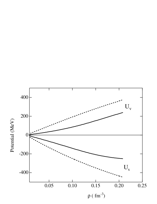
Fig. 3: The scalar and vector potentials are plotted as a function of the density for the extended chiral sigma model shown by solid curve and those for RMF(TM1) by dashed curve.

As a comparison, the energy per particle of the mean field result with the TM1 parameter set is shown together with the present result [12]. The RMF(TM1) calculation reproduces the results of the relativistic Brueckner-Hartree-Fock calculation [19]. We see that the present equation of state is much harder than the one of RMF(TM1). The incompressibility comes out to be 650 MeV, while it is 281 MeV for TM1. In Fig. 3 we plot the vector and the scalar potentials and compare with the ones of RMF(TM1). The values are about a half of the case of the TM1 parameter set. This is because the extended chiral sigma model has solutions at smaller sigma values than those for RMF(TM1).

We would like to note the consequence of the smaller absolute values of the scalar and the vector potentials in finite nuclei as shown in Fig. 3. The summation of the absolute values of the scalar and the vector potentials is directly related with the spin-orbit potential of finite nuclei. Hence, the fact that these absolute values are about a half of the values of RMF(TM1) indicates that the spin-orbit splitting for finite nuclei will come out to be about a half of the necessary spin-orbit splittings.

4 Extended chiral sigma model for finite nuclei

We are now in the position to apply the extended chiral sigma (ECS) model, which is able to provide the saturation property with the above mentioned features, to finite nuclei. For this purpose we take the N = Z even-even mass nuclei to avoid the complication coming from the isovector part of the nucleon-nucleon interaction. We calculate these nuclei using the RMF framework with the ECS Lagrangian and compare the results with those of the standard RMF calculation with the TM1 parameter set. Since the role of the pion mean field on the binding energy and the spin-orbit interaction has been demonstrated in Ref. [11] for finite nuclei, we shall introduce the RMF formalism on the treatment of the finite pion mean field and study the effect of the finite pion mean field on the nuclear properties.

We write here the RMF equations for the finite nuclei with the pion mean field. The Euler-Lagrange equation gives us the Dirac equation for the nucleon:

$$(-i{\vec{\mathchar 28939\relax}}\cdot\nabla+\mathchar 28941\relax_{0}(M+g_{\mathchar 28955\relax}\mathchar 28955\relax)+g_{\mathchar 28961\relax}\mathchar 28961\relax+\frac{g_{\rm A}}{2f_{\mathchar 28953\relax}}\mathchar 28941\relax_{0}\mathchar 28941\relax_{5}{\vec{\mathchar 28941\relax}}\cdot\mathchar 28956\relax^{0}\nabla\mathchar 28953\relax){\mathchar 28960\relax}=\mathchar 28962\relax{\mathchar 28960\relax},$$ (4.1)

and the Klein-Gordon equations for the mesons:

$$(-\nabla^{2}+{m_{\mathchar 28953\relax}}^{2})\mathchar 28953\relax = \frac{g_{\rm A}}{2f_{\mathchar 28953\relax}}\mathchar 28954\relax_{\rm pv},$$ (4.2)

$$(-\nabla^{2}+{m_{\mathchar 28955\relax}}^{2})\mathchar 28955\relax = -g_{\mathchar 28955\relax}\mathchar 28954\relax_{\rm s}-3\mathchar 28949\relax{f_{\mathchar 28953\relax}}\mathchar 28955\relax^{2}-\mathchar 28949\relax\mathchar 28955\relax^{3}+{\widetilde{g_{\mathchar 28961\relax}}}^{2}{f_{\mathchar 28953\relax}}\mathchar 28961\relax^{2}+{\widetilde{g_{\mathchar 28961\relax}}}^{2}\mathchar 28955\relax\mathchar 28961\relax^{2},$$ (4.3)

$$(-\nabla^{2}+{m_{\mathchar 28961\relax}}^{2})\mathchar 28961\relax = g_{\mathchar 28961\relax}\mathchar 28954\relax_{\rm v}-2{\widetilde{g_{\mathchar 28961\relax}}}^{2}{f_{\mathchar 28953\relax}}\mathchar 28955\relax\mathchar 28961\relax-{\widetilde{g_{\mathchar 28961\relax}}}^{2}\mathchar 28955\relax^{2}\mathchar 28961\relax,$$ (4.4)

where we consider the isospin symmetry nucleus, N = Z. There is a symmetry theorem for the Hartree-Fock (mean field) approximation with respect to the symmetry of the original Lagrangian [20, 21]. In the isospin symmetric nuclear case, we can verify that the mean field Lagrangian is symmetric under the isospin rotation to mix the proton and the neutron states. Hence, we can take a special case, where only $\mathchar 28953\relax^{0}$ is finite due to the isospin symmetry of the mean field Lagrangian and write it as $\mathchar 28953\relax$. In fact, we have checked this symmetry by performing the mean field calculations with $\mathchar 28953\relax^{0}$ in one case and with $\mathchar 28953\relax^{\pm}$ in another case and obtained the same energy in both cases [11]. We take the static approximation and assume the time reversal symmetry of the system. We have introduced here $g_{A}$ in the pion nucleon coupling in order to fulfill the Goldberger-Treiman relation. In the linear sigma model, we get $g_{A}=1$. In the mean field approximation, the source terms of the Klein-Gordon equations are replaced by their expectation values in the ground state.

$$\frac{g_{\rm A}}{2f_{\mathchar 28953\relax}}\nabla\cdot\bar{{\mathchar 28960\relax}}\mathchar 28941\relax_{5}{\vec{\mathchar 28941\relax}}\mathchar 28956\relax^{0}{\mathchar 28960\relax} \longrightarrow \frac{g_{\rm A}}{2f_{\mathchar 28953\relax}}\langle\nabla\cdot\bar{{\mathchar 28960\relax}}\mathchar 28941\relax_{5}{\vec{\mathchar 28941\relax}}\mathchar 28956\relax^{0}{\mathchar 28960\relax}\rangle=\frac{g_{\rm A}}{2f_{\mathchar 28953\relax}}\mathchar 28954\relax_{\rm pv},$$ (4.5)

$$g_{\mathchar 28955\relax}\bar{{\mathchar 28960\relax}}{\mathchar 28960\relax} \longrightarrow g_{\mathchar 28955\relax}\langle\bar{{\mathchar 28960\relax}}{\mathchar 28960\relax}\rangle=g_{\mathchar 28955\relax}\mathchar 28954\relax_{\rm s},$$ (4.6)

$$g_{\mathchar 28961\relax}\bar{{\mathchar 28960\relax}}\mathchar 28941\relax_{0}{\mathchar 28960\relax} \longrightarrow g_{\mathchar 28961\relax}\langle\bar{{\mathchar 28960\relax}}\mathchar 28941\relax_{0}{\mathchar 28960\relax}\rangle=g_{\mathchar 28961\relax}\mathchar 28954\relax_{\rm v}.$$ (4.7)

The total energy is given by

$$E_{\rm total} = \int d^{3}r{\cal H}$$

$$= \sum_{njm}\mathchar 28962\relax_{njm}-\int d^{3}r{\hbox{$\left\{\vbox to0.0pt{}\right.\n@space$}}\frac{1}{2}g_{\mathchar 28955\relax}\mathchar 28954\relax_{\rm s}\mathchar 28955\relax+\frac{1}{2}g_{\mathchar 28961\relax}\mathchar 28954\relax_{\rm v}\mathchar 28961\relax-\frac{1}{2}\frac{g_{\rm A}}{2f_{\mathchar 28953\relax}}\mathchar 28954\relax_{\rm pv}\mathchar 28953\relax$$

$$\hskip 128.0374pt+\frac{1}{6}(3\mathchar 28949\relax{f_{\mathchar 28953\relax}})\mathchar 28955\relax^{3}+\frac{\mathchar 28949\relax}{4}\mathchar 28955\relax^{4}-\frac{1}{2}{\widetilde{g_{\mathchar 28961\relax}}}^{2}f_{\mathchar 28953\relax}\mathchar 28955\relax\mathchar 28961\relax^{2}-\frac{1}{2}{\widetilde{g_{\mathchar 28961\relax}}}^{2}\mathchar 28955\relax^{2}\mathchar 28961\relax^{2}{\hbox{$\left\}\vbox to0.0pt{}\right.\n@space$}}$$

$$\hskip 213.39566pt-ZM_{\rm p}-ZM_{\rm n}-E_{\rm c.m.},$$

where we take the center of mass correction as $E_{\rm c.m.}=\frac{3}{4}(41A^{\frac{1}{3}})$ MeV. We write here the wave functions and the densities for the case of the finite pion mean field. In this case, the parity of the nucleon is broken, because the pion source term has the negative parity. The nucleon wave functions are then written as,

$$\mathchar 28960\relax_{njmm_{\mathchar 28956\relax}}=\left(\begin{array}[]{@{\,}r@{\,}}iG_{n\mathchar 28948\relax m_{\mathchar 28956\relax}}{\cal Y}_{\mathchar 28948\relax m}\mathchar 28944\relax(m_{\mathchar 28956\relax})+iG_{n\bar{\mathchar 28948\relax}m_{\mathchar 28956\relax}}{\cal Y}_{\bar{\mathchar 28948\relax}m}\mathchar 28944\relax(m_{\mathchar 28956\relax})\\ F_{n\mathchar 28948\relax m_{\mathchar 28956\relax}}{\cal Y}_{\bar{\mathchar 28948\relax}m}\mathchar 28944\relax(m_{\mathchar 28956\relax})+F_{n\bar{\mathchar 28948\relax}m_{\mathchar 28956\relax}}{\cal Y}_{\mathchar 28948\relax m}\mathchar 28944\relax(m_{\mathchar 28956\relax})\\ \end{array}\right),$$ (4.9)

where the summation over $\mathchar 28948\relax$ means the parity mixing, where $\mathchar 28948\relax$ is $\mathchar 28948\relax=-(l_{\uparrow}+1)$ for $l_{\uparrow}=j-1/2$ and $\mathchar 28948\relax=l_{\downarrow}$ for $l_{\downarrow}=j+1/2$. Using these wave functions, we can calculate all the necessary densities as,

$$\mathchar 28954\relax_{s}=\sum_{nj}W_{nj}\frac{2j+1}{4\mathchar 28953\relax}\sum_{m_{\mathchar 28956\relax}}(|G_{n\mathchar 28948\relax m_{\mathchar 28956\relax}}|^{2}-|F_{n\mathchar 28948\relax m_{\mathchar 28956\relax}}|^{2}+|G_{n\bar{\mathchar 28948\relax}m_{\mathchar 28956\relax}}|^{2}-|F_{n\bar{\mathchar 28948\relax}m_{\mathchar 28956\relax}}|^{2}),$$ (4.10)

$$\mathchar 28954\relax_{v}=\sum_{nj}W_{nj}\frac{2j+1}{4\mathchar 28953\relax}\sum_{m_{\mathchar 28956\relax}}(|G_{n\mathchar 28948\relax m_{\mathchar 28956\relax}}|^{2}+|F_{n\mathchar 28948\relax m_{\mathchar 28956\relax}}|^{2}+|G_{n\bar{\mathchar 28948\relax}m_{\mathchar 28956\relax}}|^{2}+|F_{n\bar{\mathchar 28948\relax}m_{\mathchar 28956\relax}}|^{2}),$$ (4.11)

$$\mathchar 28954\relax_{pv} = -2\sum_{nj}W_{nj}\frac{2j+1}{4\mathchar 28953\relax}$$

$$\times \sum_{m_{\mathchar 28956\relax}}(-1)^{\frac{1}{2}-m_{\mathchar 28956\relax}}{\Bigl{\{}}\frac{d}{dr}({G_{n\mathchar 28948\relax m_{\mathchar 28956\relax}}}^{\ast}G_{n\bar{\mathchar 28948\relax}m_{\mathchar 28956\relax}})+\frac{2}{r}({G_{n\mathchar 28948\relax m_{\mathchar 28956\relax}}}^{\ast}G_{n\bar{\mathchar 28948\relax}m_{\mathchar 28956\relax}})$$

$$\hskip 162.18062pt+\frac{d}{dr}({F_{n\mathchar 28948\relax m_{\mathchar 28956\relax}}}^{\ast}F_{n\bar{\mathchar 28948\relax}m_{\mathchar 28956\relax}})+\frac{2}{r}({F_{n\mathchar 28948\relax m_{\mathchar 28956\relax}}}^{\ast}F_{n\bar{\mathchar 28948\relax}m_{\mathchar 28956\relax}}){\Bigr{\}}}.$$

We are now able to calculate the coupled differential equations by doing iterative calculations.

Fig. 4: The binding energy per particle for N = Z even-even mass nuclei in the neutron number range of N = 16 $\sim$ 34. The binding energies per particle for the case of the extended chiral sigma model without and with the pion mean field are shown by the dashed and the solid lines. As a comparison, those for the RMF(TM1) are shown by the dotted line.

In this chapter, we discuss first the properties of finite nuclei in terms of the extended chiral sigma model without introducing yet the pion mean field. We show the results of binding energies per particle of N = Z even-even mass nuclei from N = 16 up to N = 34 in Fig. 4. We take all the parameters of the extended chiral sigma model as those of the nuclear matter (Figs. 2 and 3) except for $g_{\mathchar 28961\relax}$ = 7.176 instead of 7.033 for overall agreement with the RMF(TM1) results. For comparison, we calculate these nuclei within the RMF approximation without pairing nor deformation. The RMF(TM1) provides the magic numbers, which are seen as the binding energy per particle increases at N = Z = 20 and 28. On the other hand, the extended chiral sigma model without the pion mean field provides the magic number behavior only at N = Z = 18 instead of N = Z = 20.

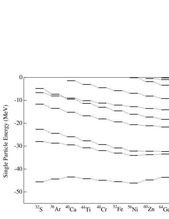
Fig. 5: The proton single particle energies for the N = Z even-even mass nuclei in the case of the RMF(TM1) theory, where the magic numbers at N = 20 and 28 are visible.

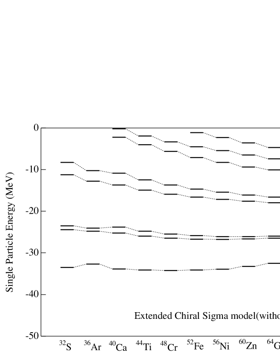
Fig. 6: The proton single particle energies for the N = Z even-even mass nuclei in the case of the extended chiral sigma model without the pion mean field. $1s_{1/2}$ orbit is pushed up and the N = 20 magic number is shifted to N = 18. The spin orbit splitting between $0f_{7/2}$ and $0f_{5/2}$ is small and the magic number at N = 28 is not visible.

In order to see why the difference between the two models for the Lagrangian arises, we show in Fig. 5 the single particle levels for the two models. In the case of the TM1 parameter set shown in Fig. 5, the shell gaps are clearly visible at N = 20 and 28. The magic number at N = 20 is due to the central potential, while the magic numbers at N = 28 comes from the spin-orbit splitting of the 0f-orbit. This is definitely due to the fact that the vector potential and the scalar potential in nuclear matter are large so as to provide the large spin-orbit splitting. On the other hand, the single particle spectrum of the extended chiral sigma model is quite different from this case as seen in Fig. 6. Most remarkable structure is that the $1s_{1/2}$ orbit is strongly pushed up. Due to this reason the $0d_{3/2}$ orbit becomes the magic shell at N = 18 and the magic number appears at N = 18 instead of N = 20. We see also not strong spin-orbit splitting and hence there appears no shell gap at N = 28. The first discrepancy could be due to the large incompressibility as seen in the nuclear matter energy per particle as seen in Fig. 2. The other is due to the relatively small vector and scalar potentials in nuclear matter as seen in Fig. 3.

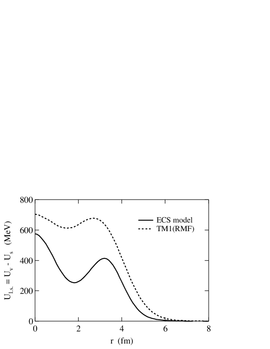
Fig. 7: The scalar-vector potential difference, $U_{ls}$, which is related with the spin-orbit potential, as a function of the radial coordinate, r. The potential difference for the case of the TM1 parameter set is shown by the dashed curve and for the ECS model is shown by the solid curve.

We would like to detail further the discussion on the spin-orbit splitting in the situation where the compressibility is very large as the ECS model, since the spin-orbit splitting is related with the behavior of the scalar-vector potential difference in the surface region. We show in Fig. 7 how the scalar-vector potential difference behaves as a function of r, which is defined as $U_{ls}=U_{V}-U_{S}$. The magnitude of the ECS model is about a half of the TM1 case. The spin-orbit potential is then defined by eliminating the small component in the relativistic wave function and by getting the spin-orbit operator explicitly as,

$$V_{ls}=\frac{2}{r}\frac{\frac{d}{dr}U_{ls}}{(M+\mathchar 28962\relax-U_{ls})^{2}}\vec{l}\cdot\vec{s}$$ (4.13)

The spin-orbit potential is proportional to the derivative of the scalar-vector potential difference, which emphasizes the contribution from the nuclear surface. Hence, to compare the magnitude of the spin-orbit effects of the two cases, we calculate the volume integrals of $V_{ls}$;

$$\int\frac{2}{r}\frac{\frac{d}{dr}U_{ls}}{(M+\mathchar 28962\relax-U_{ls})^{2}}r^{2}dr$$ (4.14)

We use for the $\mathchar 28962\relax$ the value corresponding to the binding energy of 8MeV, and obtain the ratio of the two cases as 0.48, which is again about a half. Hence, the spin-orbit effect for the ECS model is about a half of the TM1 case, which could be seen already in the single particle spectra shown in Fig. 6.

5 Finite pion mean field for finite nuclei

We include now the pion mean field in the relativistic mean field calculation[22, 23]. The method of the numerical calculation is provided in the paper of Toki et al.[11] and Sugimoto et al.[18]. The results on the binding energy per particle are shown in Fig. 4. In this calculation we take 1.15 instead of the experimental axial coupling constant $g_{\rm A}$ = 1.25 due to the Goldberger-Treimann relation. We take this smaller value in order to reproduce the binding energy for ⁵⁶Ni. It is very interesting to see that the magic number effect at N = 28 appears as the binding energy per particle increases at N = 28. This large effect of the finite pion mean field for the jj-closed shell nuclei has been demonstrated in the previous work[11].

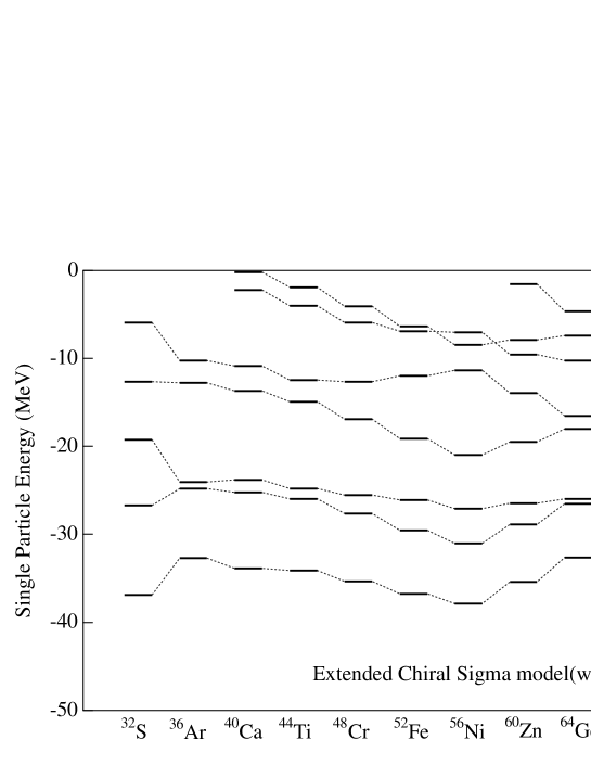
Fig. 8: The proton single particle energies for the N = Z even-even mass nuclei in the case of the extended chiral sigma model with the pion mean field. The spin-orbit splitting is made large due to the finite pion mean field, which is visible as centered at the N = Z = 28 nucleus. We note that while the total angular momentum is a good quantum number, but the angular momentum is not exact, we write the dominant angular momentum beside each single particle state.

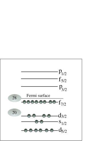
Fig. 9: The schematic picture of the single particle states and the occupied particles in the ⁵⁶Ni nucleus.

We give here an intuitive explanation to understand the energy curve of the magic structure in Fig. 4 to be given by the finite pion mean field using the schematic picture in Fig. 9. To proceed, we have to know first the effect of the finite pion mean field in terms of the shell model. The discussion of the parity projection, done in the previous publication[11], clearly shows that the pionic correlations due to the finite pion mean field is expressed by the coherent 0^- particle-hole excitations, in which the coupling of the different parity states $l$ and $l^{\prime}=l\pm 1$ with the same total spin $j$ in the shell model language. In the discussion of the contribution to the pionic correlations from various single particle states, the highest spin state in each major shell has a special role. Only this highest spin state does not find the partner to form the 0^- state in the lower major shells. However, if this state is filled by nucleons, those nucleons are able to find the 0^- partners in the higher major shells by making particle-hole excitations. Hence, the position of the highest spin state in a major shell with respect to the Fermi surface is important for the strength of pionic correlations in nuclei.

In the case of discussion, the highest spin state is the $f_{7/2}$ state as shown in Fig. 9. In the ⁴⁰Ca case, the occupied states can not couple with the $f_{7/2}$ state to form 0^- and the $f_{7/2}$ level is not used at all for the pionic correlations. In the next ⁴⁴Ti case, nucleons start to occupy the $f_{7/2}$ level, and these nucleons are used for the 0^- particle-hole excitations into $g_{7/2}$ levels. The number of particles to be used by the pionic correlation increases as the nucleon number is increased until ⁵⁶Ni, where the $f_{7/2}$ level is completely occupied. For the nuclei above ⁵⁶Ni, the upper shells as $f_{5/2}$ are to be occupied and those states are not used for 0^- particle-hole excitations from the $d_{5/2}$ level below caused by the pionic correlation due to the Pauli blocking. For ⁵⁶Ni, the pionic correlation becomes maximum. This is the reason why ⁵⁶Ni obtains the largest pionic correlation energy, which leads to the appearance of the magic number at N = 28.

We discuss now the effect of the finite pion mean field on the single particle energies. We show in Fig. 8 the single particle spectra for various nuclei. We see clearly the large energy differences between the spin-orbit partners to be produced by the finite pion mean field as the energy differences become maximum for nuclei at N = 28. The pion mean field makes coupling of different parity states with the same total spin. The $0s_{1/2}$ state repels each other with the $0p_{1/2}$ state and therefore the $0s_{1/2}$ state is pushed down and the $0p_{1/2}$ state is pushed up. The next partner is $0p_{3/2}$ and $0d_{3/2}$. The $0p_{3/2}$ state is pushed down, while the $0d_{3/2}$ state is pushed up. The next partner is $0d_{5/2}$ and $0f_{5/2}$. The $0d_{5/2}$ state is pushed down, while the $0f_{5/2}$ state is pushed up. This pion mean field effect continues to higher spin partners. This coupling of the different parity states with the same total spin due to the finite pion mean field causes the splittings of the spin-orbit partners as seen clearly for the $0p$ spin-orbit partner, $0d$ spin-orbit partner and $0f$ spin-orbit partner in ⁵⁶Ni. It is extremely interesting to see that the appearance of the energy splitting between the spin-orbit partners for the case of the finite pion mean field is caused by completely a different mechanism from the case of the spin-orbit interaction.

We would like to see the contributions of each term in the Lagrangian for the cases with and without the pion mean field in Table 1.

Table I: The binding energy per particle (BE/A) and the contributions of the sum of sigma and omega, (U${}_{\mathchar 28955\relax}+$ U_ω), kinetic (KE), pion (U_π), non-linear term (NL), sigma-omega coupling term (CP) and Coulomb (U_C) energies per nucleon in MeV for ⁵⁶Ni in the extended chiral sigma model.

	BE/A	${\rm U}_{\mathchar 28955\relax}+{\rm U}_{\mathchar 28961\relax}$	KE	${\rm U}_{\mathchar 28953\relax}$	NL	CP	${\rm U}_{\rm C}$
with $\mathchar 28953\relax$ field	8.6	-21.8	20.9	-2.9	8.1	-15.4	2.6
without $\mathchar 28953\relax$ field	8.4	-22.6	18.8	0	8.0	-15.0	2.6

The binding energy increases slightly by making the pion mean field finite. The pion term contributes attractively and the energy gain due to the pion term is obtained by making the kinetic energy and the sum of the sigma and omega potential terms increase. The structure of the wave functions changes largely, while the total energy is kept almost unchanged. This change of the structure will make the observables associated with the spin quantities change largely. The effect of the structure change on various observables will be studied in the near future.

6 Conclusion

We have studied infinite nuclear matter and finite nuclei with the nucleon number N = Z even-even mass in the range of N = 16 and N = 34 using the chiral sigma model, which is good for hadron physics. The direct application of the chiral sigma model is not able to provide the good saturation property of infinite matter. We have then used the extended chiral sigma (ECS) model, in which the omega meson mass is dynamically generated by the sigma condensation as the nucleon mass. This ECS model is able to provide a good saturation property, although the incompressibility comes out to be too large. Another characteristic property of the ECS model is that the scalar and vector potentials are about a half of the case of the RMF(TM1) model in nuclear matter.

We have then applied this ECS model to finite nuclei. The ECS model without the pion mean field gives the result that the magic number appears at N = 18 not at N = 20. This result comes from the large incompressibility found in the equation of state as K = 650 MeV. This property of the ECS model provides the mean field central potential repulsive in the interior region and the 1$s$-orbit is extremely pushed up. Due to this, the magic number appears at N = 18 instead of N = 20. We note that this problem originates from the ECS model treated in the present framework and the finite pion mean field under the mean field approximation does not remove this difficulty. There are several possibilities to be worked out to cure this problem as the effect of Dirac sea, the parity projection, and the Fock term.

The ECS model without the pion mean field provides the result that the magic number does not appear at N = 28. This result comes from another characteristic property of the ECS model, which is the small scalar and vector potentials in nuclear matter. The scalar and vector potentials lead directly to the strength of the spin-orbit interaction in finite system. Since the spin-orbit interaction given by the ECS model is about a half of those of the standard RMF calculation with the TM1 parameter set, the energy splittings between the spin-orbit partners are small and, therefore, there appears no magic effect at N = 28. As for this point, it is important to introduce the pion mean field by breaking the parity of the single particle states in the ECS model Lagrangian. Since the role of the pion mean field on the jj-closed shell nuclei has been demonstrated in the previous publication[11], we have introduced the parity mixed intrinsic single particle states in order to treat the pion mean field in finite nuclei. We followed the formulation of Sugimoto et al.[18] in the RMF framework. We have found that the magic number effect appears at N = 28. We have studied the change of the single particle spectrum due to the finite pion mean field. It is extremely interesting to find that the spin-orbit partners are split largely by the pion mean field effect. Namely, the parity partners as ($s_{1/2}$ and $p_{1/2}$), ($p_{3/2}$ and $d_{3/2}$) and ($d_{5/2}$ and $f_{5/2}$) are pushed out each other due to the pion mean field and as the consequence the spin-orbit partners are split largely like the ones of the ordinary spin-orbit splittings. This is related with the energy differences of the spin-orbit partners caused by the energy loss of the tensor (pionic) correlations due to the Pauli blocking[24].

It is gratifying to observe that first the extended chiral sigma model, which has the chiral symmetry and its dynamical symmetry breaking, is able to provide the nuclear property with only a small adjustment of the parameters in the Lagrangian. The energy splitting between the spin-orbit partners appears remarkably in the ECS model with the pion mean field. The most important consequence obtained in this study is that this energy splitting is caused by the pion mean field which is completely a different mechanism from the case of the spin-orbit interaction introduced phenomenologically. This suggests the origin of the magic effect of jj-closed shell nuclei.

References

[1] M. Gell-Mann and M. Levy, Nuovo Cimento 16 (1960), 705.
[3] Y. Nambu and G. Jona-Lasinio,
Phys. Rev. 122 (1961), 345; 124 (1961), 246.
[4] B. W. Lee, Chiral Dynamics, Gordon and Breach Science
publishers.
[5] H. Yukawa, Proc. Phys.-Math. Soc. Jpn. 17 (1935), 48.
[6] J.D. Walecka, Ann. of Phys. 83 (1974), 491; B.D. Serot and J.D. Walecka, in
Advances in Nuclear Physics, edited by J.W. Negele and
E. Vogt (Plenum Press, New York, 1986), vol. 16, p. 1.
[7] J. Boguta, Phys. Lett. 120B (1983), 34; 128B (1983), 19.
[8] J. Kunz, D. Masak, U. Post, and J. Boguta, Phys. Lett. 169B (1986), 133.
[9] V. N. Fomenko, S. Marcos, and L.N. Savushkin,J. of Phys. G19 (1993), 545.
[10] V.N. Fomenko, L.N. Savushkin, S. Marcos, R. Niembro, and M.L. Quelle,
J. of Phys. G21 (1995), 53.
[11] H. Toki, S. Sugimoto and K. Ikeda, Prog. Theor. Phys. 108 (2002), 903.
[12] Y. Sugahara and H. Toki, Nucl. Phys. A579 (1994), 557.
[13] A. Hosaka et al., to be published (2003).
[14] K. Kawarabayashi and M. Suzuki, Phys. Rev. Lett. 16 (1996), 255.
[15] A. Hosaka, Phys. Lett. 244B (1990), 363.
[16] O. Kaymakcalan, S. Rajeev, and J. Schechter, Phys. Rev. D30 (1984), 594.
[17] Riazuddin and Fayyazuddin, Phys. Rev. 147 (1966), 1071.
[18] S. Sugimoto, H. Toki, and K. Ikeda, to be published.
[19] R. Brockmann and R. Machleidt, Phys. Rev. C42 (1990), 1965.
[20] G. Ripka, Adv. Nucl. Phys. 1 (1968), 183.
[21] H. Horiuchi and K. Ikeda, Int. Rev. Nucl. Phys. 4 (1985), 1.
[22] H. Toki and W. Weise, Phys. Rev. Lett. 42 (1979), 1034.
[23] E. Oset, H. Toki, and W. Weise, Phys. Rep. 83 (1982), 281.
[24] S. Takagi, W. Watari, and M. Yasuno, Prog. Theor. Phys. 22 (1959), 549;
T. Terasawa, Prog. Theor. Phys. 23 (1960), 87; A. Arima and T. Terasawa,
Prog. Theor. Phys. 23 (1960), 115.