Improved Unitarized Heavy Baryon Chiral Perturbation Theory for $\pi N$ Scattering to fourth order

Abstract

We extend our previous analysis of the unitarized pion-nucleon scattering amplitude including up to fourth order terms in Heavy Baryon Chiral Perturbation Theory. We pay special attention to the stability of the generated $\Delta(1232)$ resonance, the convergence problems and the power counting of the chiral parameters.

I Introduction

Unitarization methods have been widely and successfully employed in the recent past to enlarge the applicability region of Chiral Perturbation Theory (ChPT) expansions, both in the meson-meson sector as well as in the meson baryon sector and to describe the lightest resonances without including them explicitly as degrees of freedom. Two important constraints are required: exact unitarity and compliance with Chiral Perturbation Theory at a given order of the expansion. In practice this approach provides a remarkable description of data in the scattering region. In the case of $\pi N$ scattering in the elastic region, the subject of this paper, a thorough partial wave analysis exists AS95 (see also the recent update Arndt:2003if ). For such a system, pions and nucleons are treated as explicit degrees of freedom and a consistent counting becomes possible if nucleons are treated as heavy particles but in a covariant framework IW89 , yielding the so called Heavy-Baryon Chiral Perturbation Theory (HBChPT) JM91 ; BK92 ; BKM95 . In this counting, the expansion for the scattering amplitude is done as a series of $e^{N}/(F^{2l}M^{N+1-2l})$ terms , with $l=1,\dots,[(N+1)/2]$, $M$ the baryon mass, and $F$ the pion decay constant. The quantity $e$ is a generic parameter with dimensions of energy constructed in terms of the pseudoscalar momenta and the velocity $v^{\mu}$ ($v^{2}=1$ ) and off-shellness $k$ of the baryons defined through the equation $p_{B}=\stackrel{{\scriptstyle\circ}}{{M}}v+k$, with $p_{B}$ the baryon four momentum and $\stackrel{{\scriptstyle\circ}}{{M}}$ the baryon mass at leading order in the expansion. After the relevant effective Lagrangian was written down EM96 , and the issue of wave function renormalization was studied Ecker:1997dn standard HBChPT calculations to second BKM97 third Mo98 ; FMS98 and fourth feme4 order have become available. The unitarization of these amplitudes of $\pi N$ scattering in the elastic region has followed closely these developments, particularly the third order calculation Mo98 ; FMS98 . This is the lowest order which generates a perturbative unitarity correction of the amplitude. The unitarization was carried out either using the standard Inverse Amplitude Method GP99 (IAM) or its improved version GNPR00  . By successful we mean the possibility of describing the data in the resonance region with parameters of natural size. The purpose of the present paper is to extend the study initiated in Ref. GNPR00 and to analyze specifically the qualitative and quantitative new effects generated by the fourth order contribution calculated in Ref. feme4 in our unitarization scheme.

Let us then specify the scope and motivations of our work: First, our scheme is based on two fundamental ideas: demanding exact unitarity and considering the $F^{-2}$ HBChPT expansion independent from and converging faster than the $M^{-1}$ one. In GNPR00 we showed that this allows to generate the $\Delta(1232)$ as well as to fit the remaining $S$ and $P$ wave channels with natural values for the low-energy constants (LEC) unlike for instance the IAM GP99 . Our method was implemented in GNPR00 with the first contribution of order $F^{-4}$ only, coming from the third order amplitude. Including the fourth order will allow us to check the convergence of our method by considering, for instance, the ${\cal O}(F^{-4}M^{-1})$, to be included in the third order $F^{-4}$ term.

Second, there is an interesting issue that we did not account for in GNPR00 which has to do with the separation of the dimensionful third and fourth order LEC into two pieces contributing to the orders $F^{-2}$ and $F^{-4}$. As we will see below, taking into account this effect may change considerably our description of the partial waves. The reason why we did not consider it in GNPR00 is that we used the amplitudes in Mo98 , which provide an specific separation that turns out to be very natural, as we will see below .

Third, comparing the perturbative results to order three FMS98 and four feme4 , one observes that in order to achieve a reasonable convergence, the fourth order constants become of unnatural size and, furthermore, their particular values are often incompatible from one fit to another. This is a signal of the bad convergence of the HBChPT series and could influence also the convergence of our unitarized formula.

Fourth, unitarization methods are rarely applied beyond the leading order in the imaginary part of the amplitudes Nieves:2001de ; Dobado:2001rv . The study of the fourth order of $\pi N$ system within HBChPT provides an opportunity to learn about the unitarization approach beyond this lowest order.

For comparison purposes with previous works BKM97 ; Mo98 ; FMS98 ; feme4 ; GP99 ; GNPR00 we will take the partial wave analysis performed in Ref. AS95 . The recent update Arndt:2003if does not bring significant changes to our discussion.

II The unitarized amplitude

In order to have a neat separate expansion of the partial waves in powers of $M^{-1}$ and $F^{-2}$, we need to re-expand the amplitudes in feme4 , as it was already done to third order in GNPR00 with those in Mo98 . Then, following the notation in GNPR00 , we have, to fourth order, for any partial wave

$$f_{l\,\pm}^{(1)\,\pm} = {m\over F^{2}}t_{l\,\pm}^{(1,1)\,\pm}\Big{(}{\omega\over m}\Big{)}$$

$$f_{l\,\pm}^{(2)\,\pm} = {m^{2}\over F^{2}M}t_{l\,\pm}^{(1,2)\,\pm}\Big{(}{\omega\over m}\Big{)}$$

$$f_{l\,\pm}^{(3)\,\pm} = {m^{3}\over F^{2}M^{2}}t_{l\,\pm}^{(1,3)\,\pm}\Big{(}{\omega\over m}\Big{)}+{m^{3}\over F^{4}}t_{l\,\pm}^{(3,3)\,\pm}\Big{(}{\omega\over m}\Big{)}$$

$$f_{l\,\pm}^{(4)\,\pm} = {m^{4}\over F^{2}M^{3}}t_{l\,\pm}^{(1,4)\,\pm}\Big{(}{\omega\over m}\Big{)}+{m^{4}\over F^{4}M}t_{l\,\pm}^{(3,4)\,\pm}\Big{(}{\omega\over m}\Big{)}$$ (1)

with $m$ the pion mass, $M$ the nucleon mass, $F$ the pion decay constant and $\omega$ the pion CM energy. The partial wave unitarity condition

$${\rm Im}f_{l\,\pm}^{-1}=-q,$$ (2)

where $q$ is the CM momentum, implies that perturbatively one has 

$${\rm Im}\,t_{l\,\pm}^{(1,1)\,\pm}={\rm Im}\,t_{l\,\pm}^{(1,2)\,\pm} = {\rm Im}\,t_{l\,\pm}^{(1,3)\,\pm}=0$$

$${\rm Im}\,t_{l\,\pm}^{(3,3)\,\pm} = {q\over m}\left[t_{l\,\pm}^{(1,1)\,\pm}\right]^{2}$$

$${\rm Im}\,t_{l\,\pm}^{(3,4)\,\pm} = 2{q\over m}t_{l\,\pm}^{(1,1)\,\pm}t_{l\,\pm}^{(1,2)\,\pm}$$ (3)

Following the same ideas as in GNPR00 , we will consider the unitarized amplitude to fourth order:

$${1\over f|_{\rm Unitarized}} = {F^{2}\over m}{1\over t^{(1,1)}+{m\over M}\,t^{(1,2)}+\,({m\over M})^{2}\,t^{(1,3)}+\,({m\over M})^{3}\,t^{(1,4)}}-m{{t^{(3,3)}+{m\over M}t^{(3,4)}}\over[t^{(1,1)}]^{2}+2{m\over M}t^{(1,1)}t^{(1,2)}}$$ (4)

which, using (3) yields immediately (2). Let us recall that our Improved IAM formula at third order read GNPR00 :

$${1\over f|_{\rm Unitarized}} = {F^{2}\over m}{1\over t^{(1,1)}+{m\over M}\,t^{(1,2)}+\,({m\over M})^{2}\,t^{(1,3)}}-m{{t^{(3,3)}}\over[t^{(1,1)}]^{2}}$$ (5)

which can be now reobtained from eq.(4) by removing the $t^{(1,4)}$ and $t^{(3,4)}$ terms and, consistently with unitarity, removing also the $2(m/M)t^{(1,1)}t^{(1,2)}$ factor in the second denominator. Hence, as we have stressed in the introduction, the knowledge of $t^{(1,4)}$ and $t^{(3,4)}$ allows us to test our power counting by including one more term both in the ${\cal O}(F^{-2})$ and ${\cal O}(F^{-4})$ contributions.

III The third order and the LEC power counting

In the literature there are two $O(q^{3})$ calculations Mo98 ; FMS98 , using different choices of counterterms and renormalization schemes, but only one at $O(q^{4})$ feme4 following the FMS98 scheme. The translation between them does not simply amount to a change of notation, but involves some $1/M$ corrections. Since our results at third order GNPR00 were constructed directly from Mo98 , we have to check to what extend our previous ${\cal O}(q^{3})$ results are reproduced when using the amplitudes and notation of Refs. FMS98 ; feme4 . In so doing two remarks are in order:

First, already at third order, the re-expanded amplitudes of Mo98 and FMS98 differ slightly due both to a different choice of the reference frame and of the nucleon wave function renormalization (see comments in FMS98 ). In practice, this just means that there are slight numerical differences between the perturbative results, which eventually could be absorbed in the numerical values of the LEC of the HBChPT Lagrangian.

A second point becomes more relevant for our purposes: if we just take the third order amplitudes in FMS98 , we re-expand them separating the different contributions and use our third order unitarized formula (eq.(13) in GNPR00 ), we find a much worse result than in GNPR00 , particularly in the P33 channel where the $\Delta(1232)$ resonance should appear. This is shown in Figure 1a. We remark that we are using a set of parameters compatible with those in GNPR00 , where the description of the resonance was excellent within the errors even without fitting.

The origin of this apparent discrepancy is that we have not taken into account that in our power counting scheme, the LEC themselves may have contributions of different orders. In fact, all the difference with GNPR00 is that we have chosen now a different parametrization of LEC, although the numerical values are compatible: in GNPR00 we followed EM96 ; Mo98 where the five ${\cal O}(q^{3})$ LEC appearing in the amplitude are called $b_{1}+b_{2},b_{3},b_{6},b_{16}-b_{15},b_{19}$. Here, we follow FMS98 ; feme4 where the relevant ${\cal O}(q^{3})$ constants are $\bar{d}_{1}+\bar{d}_{2},\bar{d}_{3},\bar{d}_{5},\bar{d}_{14}-\bar{d}_{15},\bar{d}_{18}$. Comparing the Lagrangian given in equations (2.45)-(2.47) of FMS98 with that in EM96 one observes that the $b_{i}$ are related to the $\bar{d}_{i}$ for $i=1,2,3$ and to the $\bar{d}_{i-1}$ for $i=6,15,16,19$ typically as:

$$M^{2}\bar{d}_{i}\sim constant+b_{i}M^{2}/(16\pi^{2}F^{2})$$ (6)

with a constant that is ${\cal O}(1)$ in the $F^{-2}$ counting. This comes from the fact that in EM96 some finite terms coming from renormalization have been absorbed in the $b_{i}$.

Now, following our power counting arguments, if we replace in the amplitudes of refs.FMS98 ; feme4 the $\bar{d}_{i}$ using eq.(6), there are pieces in $t^{(1,3)}$ shifted to $t^{(3,3)}$ (remember that all the dependence with the $\bar{d}_{i}$ is in $t^{(1,3)}$). This changes the functional dependence of $t^{(3,3)}$, including, for instance, higher order polynomial contributions that otherwise were not present. Although the perturbative amplitude remains the same, the unitarized one changes since $t^{(1,3)}$ and $t^{(3,3)}$ are treated on a different footing. With this procedure we obtain the unitarized results shown in Figure 1b. The improvement is clear for the P33 wave and the results are similar to those in GNPR00 . The corresponding values for the mass and width of the $\Delta(1232)$ extracted from the phase shifts are given in the second column of Table 1. This highlights the importance of taking into account the counting of the LEC.

The above separation is, of course, arbitrary, since nothing prevents us from normalizing the $\bar{d}_{i}$, which are quantities of dimension $E^{-2}$ as $(4\pi F^{2})\bar{d}_{i}$ instead of $M^{2}\bar{d}_{i}$, assuming that both are quantities of natural size. Thus, the most general way to proceed would be to consider as free parameters the coefficients of the ${\cal O}(1)$ and ${\cal O}(F^{-2})$ terms in $M^{2}\bar{d}_{i}$. In such a way we would duplicate the number of ${\cal O}(q^{3})$ LEC, rendering the approach unnecessarily complicated, since we already know that it is enough to consider the separation given by the $b_{i}$ parametrization EM96 . We will thus use only that separation in our calculations, but, after performing the fit, we will give the results in the $\bar{d}_{i}$ set for easier comparison with the literature.

The results of our ${\cal O}(q^{3})$ fit is shown in Figure 2. The fit parameters and their errors are given in the fourth column of Table 3 whereas the results for the $\Delta$ mass and width are given in Table 1. All them are in agreement with what we found in GNPR00 . The description of data in all channels is very good and our ${\cal O}(q^{3})$ LEC are all of natural size although, as it also happened in GNPR00 , they differ somewhat from those obtained from HBChPT (second column in Table 3). Note that systematic errors are not given in Table III, although they are dominant as it can be seen from Table II). This is probably another consequence of the poor convergence of the HBChPT series. Let us nevertheless recall that, in GNPR00 it was shown that one can perform ${\cal O}(q^{3})$ fits where the ${\cal O}(q^{2})$ parameters $c_{i}$ are fixed to the predictions of Resonance Saturation BKM97 and the results are still in excellent agreement with data.

,

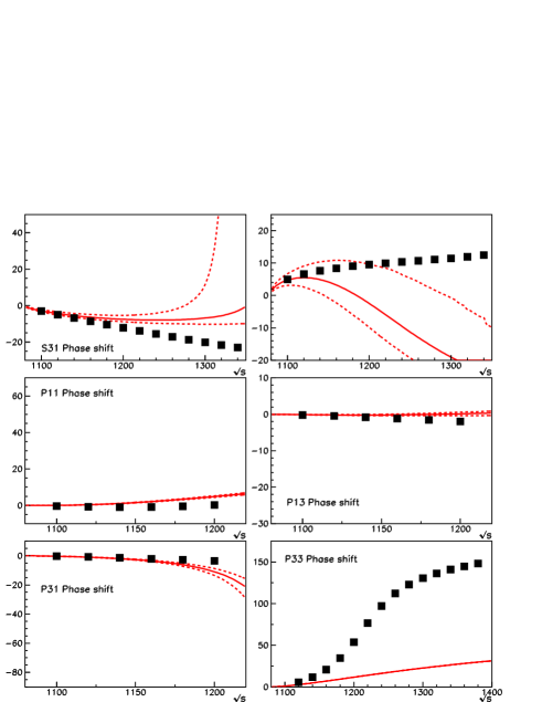
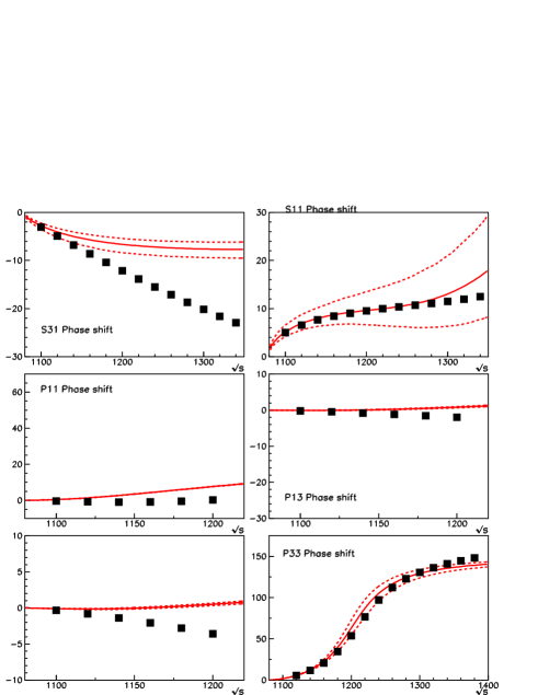
Figure 1: ${\cal O}(q^{3})$ Unitarized phase shifts as a function of the total CM energy $\sqrt{s}$: As explained in section III: a) In the two left columns we use the $\bar{d}_{i}$, whereas in b) in the two right columns we use the $b_{i}$ set. Experimental data are from AS95 . The areas between dotted lines correspond to the propagated errors of the parameters of fit 1 in  FMS98 in both cases.

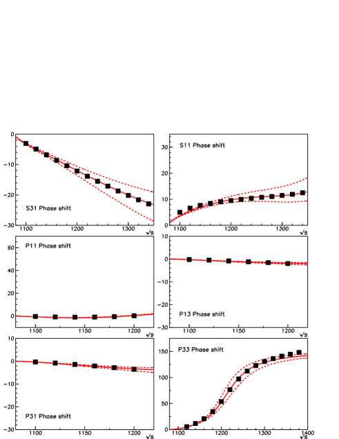
Figure 2: Unitarized ${\cal O}(q^{3})$ fit. The fit parameters are given in Table 3. The areas between dotted lines correspond to the errors given in Table 3.

IV Fourth order results

Let us consider now our fourth order unitarized amplitude (4) with the HBChPT amplitudes of feme4 . In principle, the ${\cal O}(q^{4})$ amplitude depends on nine different combinations of ${\cal O}(q^{4})$ constants $\bar{e}_{i}$, in addition to the four ${\cal O}(q^{2})$ $c_{i}$ and the five ${\cal O}(q^{3})$ $\bar{d}_{i}$. These nine combinations are displayed in the first column of Table 3. However, as noted in feme4 , the last four combinations actually amount to renormalize the $c_{i}$, giving rise to new $\tilde{c}_{i}$ as given in eq.(3.23) of feme4 . Strictly speaking, the ${\cal O}(q^{4})$ amplitude depends on 18 parameters, since the $c_{i}$ still appear in the pure ${\cal O}(q^{4})$ terms. However, replacing those $c_{i}$ by $\tilde{c}_{i}$ introduces higher order corrections, so that the number of free parameters up to ${\cal O}(q^{4})$ is really 14. At this point, as commented in feme4 one can follow two different strategies. The first one is to consider as free parameters $\tilde{c}_{i},\bar{d}_{i}$ and the $\bar{e}_{i}$ with $i=14-18$. This is the parameter set listed in Table 2. Although this is the more natural set, it has the inconvenience that one cannot disentangle which part of the $\tilde{c}_{i}$ comes from ${\cal O}(q^{4})$ renormalization, since those corrections are relatively large (another signal of the HBChPT bad convergence). As a consequence, it becomes more difficult to compare with previously published values for the $c_{i}$. The alternative (strategy 2) is to fix the $c_{i}$ values, which in turn are the ones less subjected to uncertainties and then use the $\bar{d}_{i}$ and the nine combinations of $\bar{e}_{i}$ as free parameters. This second strategy is useful for instance to fix the $c_{i}$ to the predictions of Resonance Saturation BKM97 as we also did in GNPR00 .

In addition, we have to face again the problem of the LEC counting, according to the discussion in the previous section. Thus, besides the “reordering” of terms coming from the $\bar{d}_{i}$, we now have to consider also that coming from the separation of $M^{3}\bar{e}_{i}$ into a constant (a contribution to $t^{(1,4)}$) plus an ${\cal O}\left(M^{2}/(4\pi F)^{2}\right)$ term (which contributes to $t^{(3,4)}$). Recall that in this case we do not have any “natural” way to perform that separation, as in the ${\cal O}(q^{3})$ case.

IV.1 The unitarized partial waves to ${\cal O}(q^{4})$

First, as we did to ${\cal O}(q^{3})$, we will show the predictions of our formula without fitting, performing a Monte Carlo sampling of the perturbative LEC, assuming that they are uncorrelated. Following the first strategy, we have used the LEC given in feme4 , in particular those given in their “Fit 3” that we reproduce in Table 2. We also list the “Fit 1 and 2” parameter sets to illustrate that, as pointed out in feme4 , the systematic errors are much larger than the statistical ones, that we are quoting in the Table. For that reason we will take bigger errors, since the errors listed in feme4 are clearly underestimated. In view of the uncertainties in feme4 we have assigned an error of $1.0$ to $\bar{e}_{14},\bar{e}_{15},\bar{e}_{17},\bar{e}_{18}$, of $0.5$ to $\tilde{c}_{1}$, $\tilde{c}_{2}$, $\tilde{c}_{3}$ (the $\tilde{c}_{i}$ have bigger uncertainties than the $c_{i}$ due to their $\bar{e}_{i}$ contribution) and of $0.25$ to the remaining LEC. In Figure 3a we show the ${\cal O}(q^{4})$ prediction “redefining” the $\bar{d}_{i}$ as before but without doing so for the $\bar{e}_{i}$, while in Figure 3b we have also redefined the $\bar{e}_{i}$ for convenience as $M^{3}\bar{e}_{i}=1+\bar{f}_{i}M^{2}/(4\pi F)^{2}$. Throughout this paper, and for practical purposes, we will consider only these two situations.

,

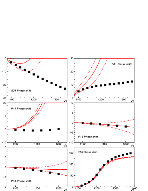
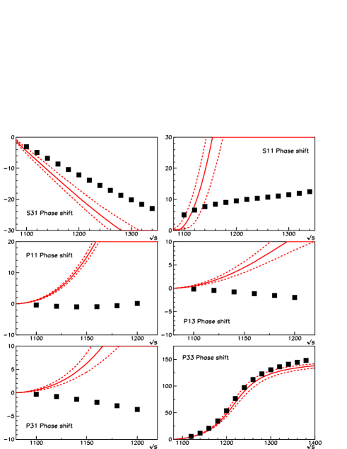
Figure 3: ${\cal O}(q^{4})$ Unitarized phase shifts as a function of the total CM energy $\sqrt{s}$. a) The two left columns correspond to reordering the $\bar{d}_{i}$ only, whereas b) in the two right columns we have reordered both $\bar{d}_{i}$ and $\bar{e}_{i}$. Experimental data are from AS95 . The areas between dotted lines correspond to the propagated errors of the parameters of fit 3 in  feme4 with bigger errors (see Sect.IV.a)

In view of Figure 3 there are several comments in order: First, consider the P33 channel, where our approach is meant to be more accurate. Here our ${\cal O}(q^{4})$ result confirms the ${\cal O}(q^{3})$ one and even improves it slightly. Observe for instance the results for the $\Delta$ parameters given in the fourth column of Table 1, corresponding to Figure 3b. This is one of the main conclusions of this work, namely that the ${\cal O}(q^{4})$ calculation confirms that our unitarization method generates dynamically the $\Delta(1232)$ resonance. The improvement of the P33 channel description is also a common feature with feme4 . Note also that this conclusion does not change by using the $\bar{e}_{i}$ or the $\bar{f}_{i}$ formulas as long as we redefine the ${\cal O}(q^{3})$ LEC as before.

As for the other channels, we see no actual improvement when comparing with the unfitted ${\cal O}(q^{3})$ in Figure 1b. On the contrary, we get worse results for most of them, especially the two $S$ channels and the $P_{11}$ one. Here, we see significant differences between using the $\bar{f}_{i}$ prescription or not. In fact, without fitting, our choice for the $\bar{f}_{i}$ does not seem to give better results than using the $\bar{e}_{i}$ directly (Figure 3a) or, equivalently, neglecting the ${\cal O}(F^{-2})$ contribution in $M^{3}\bar{e}_{i}$.

The hope is that we can perform ${\cal O}(q^{4})$ fits which improve these five channels without spoiling the P33 one and with a reasonable size for the LEC. However, we must bear in mind that, as commented before, the low-energy ${\cal O}(q^{4})$ fits performed in feme4 already show that one gets only slightly better descriptions and bigger uncertainties for the LEC than the ${\cal O}(q^{3})$.

	${\cal O}(q^{3})$ unfitted	fit ${\cal O}(q^{3})$	${\cal O}(q^{4})$ unfitted	fit ${\cal O}(q^{4})$	PDG
$M_{\Delta}$ (MeV)	1221 ${}^{+11}_{-10}$	1229 ${}^{+14}_{-12}$	1238${}^{+10}_{-9}$	1232${}^{+35}_{-29}$	1230 - 1234
$\Gamma_{\Delta}$ (MeV)	111.2${}^{+16.9}_{-14.3}$	108.4 ${}^{+20.6}_{-16.5}$	125.2${}^{+20.4}_{-16.4}$	107.3 ${}^{+45.1}_{-31.0}$	115-125

Table 1: $\Delta(1232)$ resonance parameters in the different cases considered in this paper. The resonance mass and width are obtained from the condition $\delta^{1}_{33}|_{s=M_{\Delta}^{2}}=\pi/2$ and $1/\Gamma_{\Delta}=M_{\Delta}(d\delta^{1}_{33}/ds)|_{s=M^{2}_{\Delta}}$.

IV.2 ${\cal O}(q^{4})$ fits

In Figure 4a we show the result of our best fit with the fit errors propagated. Here we have followed the first strategy and we have used the $\bar{f}_{i}$ defined in the previous section. The LEC and their errors are given in the last column in Table 2. The main observation is that we reproduce the data with constants of natural size. The constant $\bar{e}_{18}$ turns out to be highly correlated numerically with $\bar{e}_{17}$ so that we have chosen to fix one of them to the perturbative value. For the $\Delta$ parameters we get the results in the fifth column in Table 1 which is still fully compatible with the experimental result. Note that, as expected from our previous comments, the uncertainties in the fit parameters are now bigger than in the ${\cal O}(q^{3})$ fit. However, the quality of the fit is comparable if not better: we get a $\chi^{2}/d.o.f\sim 0.3$ for the ${\cal O}(q^{3})$ fit in Figure 2 and $\chi^{2}/d.o.f\sim 0.17$ for that in Figure 4a. As is customarily done FMS98 ; GNPR00 , for the $\chi^{2}$ calculation we havee added some error to the data; in particular, we have chosen to add a 3% relative error plus one degree systematic error. Therefore, our method shows clear signs of convergence when we perform unconstrained fits, although the uncertainties in the LEC remind us of the bad convergence of the HBChPT series. Note also that the bigger uncertainties are in the $S$ channels, as we have commented before.

We also show, in Figure 4b, the result of a fit using the second strategy and fixing the $c_{i}$ as the central values of the predictions of Resonance Saturation BKM97 . As it also happened with the ${\cal O}(q^{3})$ in GNPR00 , the fit result is slightly worse when the $c_{i}$ are not free parameters. Here we obtain a better fit when using directly the $\bar{e}_{i}$ and not the $\bar{f}_{i}$ as free ${\cal O}(q^{4})$ parameters. Nevertheless, some of the constants become of unnatural size and also the errors are bigger than for the unconstrained fit. For the fit in Figure 4b we get a $\chi^{2}/d.o.f\sim 0.58$ and the LEC listed in the fifth column in Table 3. The correlations between the different LEC also become more important. Here, in addition to $\bar{e}_{17}$ and $\bar{e}_{18}$, there are also strong correlations among $\bar{e}_{14}$, $\bar{e}_{15}$, $\bar{e}_{16}$, $\bar{e}_{22}-4\bar{e}_{38}$, $\bar{e}_{20}+\bar{e}_{35}-g_{A}\bar{d}_{16}/(8M)$, $2\bar{e}_{21}-\bar{e}_{37}$ and $2\bar{e}_{19}-\bar{e}_{22}-\bar{e}_{36}$ which allow to fix one of them. It should be commented that one could find fits with more natural values and a higher $\chi^{2}/d.o.f$ but we have preferred to show the best fit, emphasizing the convergence problems.

,

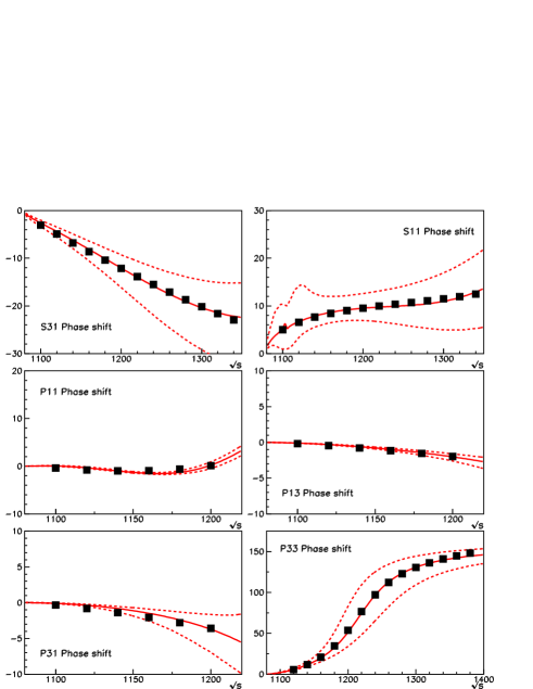
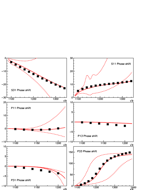
Figure 4: Unitarized ${\cal O}(q^{4})$ fits: a) using strategy 1 in the two left columns and b) using strategy 2 in the two right columns. Experimental data are from AS95 . The fit parameters and errors are given in Tables 2 and 3 respectively. The areas between dotted lines correspond to propagating those errors.

	Fettes-Meißner feme4			Our IAM
	Fit 1	Fit 2	Fit 3	${\cal O}(q^{4})$ fit
$\tilde{c}_{1}$	$-2.54\pm 0.03$	$-0.27\pm 001$	$-$3.31$\pm$ 0.03	$-$ 1.43 $\pm$ 0.10
$\tilde{c}_{2}$	$0.60\pm 0.04$	$3.29\pm 0.03$	0.13 $\pm$ 0.03	$-$ 0.33 $\pm$ 0.10
$\tilde{c}_{3}$	$-8.86\pm 0.06$	$-1.44\pm 0.03$	$-$10.37 $\pm$ 0.05	$-$ 2.62 $\pm$ 0.17
$\tilde{c}_{4}$	$2.80\pm 0.13$	$3.53\pm 0.08$	2.86$\pm$0.10	0.64$\pm$0.10
$\bar{d}_{1}+\bar{d}_{2}$	$5.68\pm 0.09$	$4.45\pm 0.05$	5.59$\pm$ 0.06	1.11 $\pm$ 1.02
$\bar{d}_{3}$	$-4.82\pm 0.09$	$-2.96\pm 0.05$	$-$4.91$\pm$0.07	$-$0.59$\pm$1.06
$\bar{d}_{5}$	$-0.09\pm 0.06$	$-0.95\pm 0.03$	$-$0.15$\pm$0.05	$-$0.19 $\pm$ 0.40
$\bar{d}_{14}-\bar{d}_{15}$	$-10.49\pm 0.18$	$-7.02\pm 0.11$	$-$11.14 $\pm$ 0.11	2.49 $\pm$1.93
$\bar{d}_{18}$	$-1.53\pm 0.17$	$-0.97\pm 0.11$	$-$0.85$\pm$0.06	$-$ 17.49$\pm$ 1.31
$\bar{e}_{14}$	$6.39\pm 0.27$	$-4.68\pm 0.14$	7.83$\pm$0.23	1.58 $\pm$ 0.53
$\bar{e}_{15}$	$4.65\pm 0.31$	$-18.41\pm 0.15$	9.72$\pm$0.25	$-$ 1.41 $\pm$ 1.13
$\bar{e}_{16}$	$7.05\pm 0.30$	$7.79\pm 0.15$	6.42$\pm$ 0.25	3.50 $\pm$ 1.30
$\bar{e}_{17}$	$4.88\pm 0.98$	$-17.79\pm 0.53$	5.47$\pm$ 0.64	6.56 $\pm$ 1.92
$\bar{e}_{18}$	$-9.15\pm 0.98$	$19.66\pm 0.53$	$-$0.17$\pm$0.64	$-$0.17 (fixed)

Table 2: HBChPT low energy constants with strategy 1. The $c_{i}$, $\bar{d}_{i}$ and $\bar{e}_{i}$ are given in GeV^-1,GeV^-2 and GeV^-3 respectively. We list the three parameter sets provided in feme4 to illustrate the large systematic uncertainties already existing in the perturbative determinations.

	Fettes et al. FMS98	Fettes-Meißner feme4	${\cal O}(q^{3})$ fit	${\cal O}(q^{4})$ fit
		${\cal O}(q^{4})$ (Strategy 2)		RS $c_{i}$ of BKM97
$c_{1}$	$-$1.53$\pm$ 0.18	$-$1.47 (input)	$-$0.43 $\pm$ 0.04	$-$0.9 (input)
$c_{2}$	3.22 $\pm$ 0.25	3.26 (input)	1.28$\pm$0.03	3.9 (input)
$c_{3}$	$-$6.20$\pm$ 0.09	$-$6.14 (input)	$-$3.10 $\pm$ 0.05	$-$5.3 (input)
$c_{4}$	3.51$\pm$0.04	3.50 (input)	$1.51\pm$0.04	3.7 (input)
$\bar{d}_{1}+\bar{d}_{2}$	$2.68\pm 0.15$	$4.90\pm 0.05$	$2.66\pm 0.20$	10.36 $\pm$0.53
$\bar{d}_{3}$	$-$3.11$\pm$0.79	$-$4.19$\pm$0.07	$-0.32\pm 0.2$	$-$ 4.07 $\pm$0.26
$\bar{d}_{5}$	0.43$\pm$0.49	$-0.16\pm 0.05$	$-1.66\pm 0.10$	$-$ 3.23 $\pm$ 0.31
$\bar{d}_{14}-\bar{d}_{15}$	$-5.74\pm 0.29$	$-9.31\pm 0.10$	$-5.34\pm 0.40$	$-$1.17 $\pm$ 0.68
$\bar{d}_{18}$	$-$0.83$\pm$0.06	$-$0.84$\pm$0.06	$-2.60\pm$0.20	$-$ 53.29 $\pm$ 3.37
$\bar{e}_{14}$		$4.19\pm 0.23$		2.24 $\pm$ 0.94
$\bar{e}_{15}$		$4.54\pm 0.25$		$-$ 2.17 $\pm$ 2.14
$\bar{e}_{16}$		$2.74\pm 0.24$		5.12 $\pm$ 1.26
$\bar{e}_{17}$		$7.20\pm 0.64$		$-$ 0.95 $\pm$ 1.86
$\bar{e}_{18}$		$-$ 3.36$\pm$0.64		$-$ 3.36 (fixed)
$\bar{e}_{22}-4\bar{e}_{38}$		27.72$\pm$0.74		27.72 (fixed)
$\bar{e}_{20}+\bar{e}_{35}-g_{A}\bar{d}_{16}/(8M)$		$-$17.35$\pm$0.36		$-$ 70.11 $\pm$ 3.07
$2\bar{e}_{19}-\bar{e}_{22}-\bar{e}_{36}$		$-25.12\pm 0.69$		97.14 $\pm$ 10.00
$2\bar{e}_{21}-\bar{e}_{37}$		$-$5.00$\pm$1.43		17.64 $\pm$10.7

Table 3: HBChPT low energy constants with strategy 2. The $\tilde{c}_{i}$, $\bar{d}_{i}$ and $\bar{e}_{i}$ are given in GeV^-1,GeV^-2 and GeV^-3 respectively.

V Conclusions

In this work we have used a unitarized $\pi N$ scattering amplitude including up to ${\cal O}(q^{4})$ terms in the standard Heavy Baryon Chiral Perturbation Theory expansion. This has allowed to test our method of considering the $F^{-2}$ expansion resumming the $M^{-1}$ contributions. The description of the $P33$ channel and the $\Delta$ resonance, which is dynamically generated, are excellent within the experimental errors. The inclusion of the new ${\cal O}(q^{4})$ terms does not change much this picture, which is a consistency check of our formalism.

In order to describe accurately the data in the other three $P$ channels and the two $S$ ones, one needs to fit the LEC. We have showed that it is possible to fit the six channels simultaneously with natural values for the LEC, although with considerably larger uncertainties than in the ${\cal O}(q^{3})$. This is a consequence of the poor HBChPT convergence which shows up already at the pure perturbative level at lower energies. In fact, when one tries to perform ${\cal O}(q^{4})$ fits constraining the lowest order constants to the Resonance Saturation hypothesis, some of the LEC become of unnatural size and their errors increase considerably. These convergence problems are especially important in the two $S$ waves.

We have also discussed the issue of the LEC power counting, which is relevant in our expansion scheme. The importance of this effect has been especially highlighted in the $P33$ channel, where a correct splitting of the ${\cal O}(q^{3})$ constants is crucial. To ${\cal O}(q^{4})$ the influence of such LEC reordering is smaller as far as the resonance is concerned, although it may improve the convergence in the other channels.

In summary, our unitarization method is robust and is almost not affected by the HBChPT convergence problems as far as the generation of the $\Delta(1232)$ resonance is concerned. However, the predictions of the unitarized amplitude to fourth order for other channels show similar problems of convergence as the perturbative one, even though one can still find excellent descriptions of data with natural values for the low-energy constants. It seems a natural continuation of this work to implement our unitarization methods within the context of the Lorentz invariant formalism proposed in bele (see also Ref. Gegelia:1999qt ) which has better convergence properties.

- (1) R.A. Arndt, I.I. Strakovsky, R.L. Workman, and M.M. Pavan, Phys. Rev. C52, 2120 (1995). R. Arndt et al. nucl-th/9807087. SAID online-program.(Virginia Tech Partial-Wave Analysis Facility). Latest update, http://gwdac.phys.gwu.edu
- (2) R. A. Arndt, W. J. Briscoe, I. I. Strakovsky, R. L. Workman and M. M. Pavan, arXiv:nucl-th/0311089.
- (3) N. Isgur and M.B. Wise, Phys. Lett. B232 (1989) 113.
- (4) E. Jenkins and A. V. Manohar, Phys. Lett. B255 (1991) 558.
- (5) V. Bernard, N. Kaiser, J. Kambor and U. -G. Meißner, Nucl. Phys. B388 (1992) 315.
- (6) For a review see e.g. V. Bernard, N. Kaiser and U.-G. Meißner, Int. J. Mod. Phys. E4 (1995) 193 and references therein.
- (7) G.Ecker and M.Mojzis, Phys.Lett. B365 (1996) 312-318.
- (8) G. Ecker and M. Mojzis, Phys. Lett. B 410, 266 (1997)
- (9) V. Bernard, N. Kaiser and U.-G. Meißner, Nucl. Phys. A615 (1997) 483.
- (10) M. Mojzis, Eur. Phys. Jour. C2 (1998) 181.
- (11) N. Fettes, U.-G. Meißner and S. Steininger, Nucl.Phys. A640 (1998) 199.
- (12) N.Fettes, U. -G. Meißner, Nucl.Phys.A676 311-338 (2000).
- (13) A. Gómez Nicola and J. R. Peláez, Phys.Rev.D62:017502,2000.
- (14) A.Gómez Nicola, J.Nieves, J.R.Peláez, E.Ruiz Arriola, Phys.Lett. B486, 77-85 (2000).
- (15) J. Nieves and E. Ruiz Arriola, Phys. Rev. D 63, 076001 (2001)
- (16) A. Dobado and J. R. Pelaez, Phys. Rev. D 65 (2002) 077502
- (17) J. Nieves, M. Pavon Valderrama and E. Ruiz Arriola, Phys. Rev. D 65 (2002) 036002
- (18) T.Becher and H.Leutwyler, Eur.Phys.J.C9 (1999) 643-671; JHEP 0106:017 (2001).
- (19) J. Gegelia, G. Japaridze and X. Q. Wang, J. Phys. G 29 (2003) 2303 [arXiv:hep-ph/9910260].