Nucleon-nucleon interaction in the $J$-matrix inverse scattering approach and few-nucleon systems

Abstract

The nucleon-nucleon interaction is constructed by means of the $J$-matrix version of inverse scattering theory. Ambiguities of the interaction are eliminated by postulating tridiagonal and quasi-tridiagonal forms of the potential matrix in the oscillator basis in uncoupled and coupled waves, respectively. The obtained interaction is very accurate in reproducing the $NN$ scattering data and deuteron properties. The interaction is used in the no-core shell model calculations of ³H and ⁴He nuclei. The resulting binding energies of ³H and ⁴He are very close to experimental values.

I Introduction

The nucleon-nucleon ($NN$) interaction is one of the most important ingredients in microscopic nuclear structure studies. Ideally, the $NN$ interaction should be derived from the quark-gluon theory. The modern status of QCD, however, makes it possible to predict reaction cross sections only at high enough energies; the QCD-based derivation of the $NN$ potential describing the nucleon-nucleon interaction at the low energies that are of primary importance for nuclear physics applications is impossible at the moment.

Nucleon-nucleon potentials conventionally referred to as ‘realistic’, are derived from the meson exchange theory. Modern realistic $NN$ potentials like Bonn Bonn , Argonne Argonne , Nijmegen Stocks , etc., are carefully fitted to the existing experimental data on $NN$ scattering and deuteron properties. Unfortunately, none of the known $NN$ interactions provides a completely satisfactory description of the trinucleon and other light nuclei. To overcome this deficiency, meson exchange TM or phenomenological Argonne-3 three-nucleon forces are usually introduced. Impressive progress was achieved recently in the description of the trinucleon and ⁴He binding energies with realistic $NN$ and three-nucleon forces alpha-3 . However, the three-nucleon force parameters in such studies are sometimes fitted to the trinucleon binding and some of them may not be consistent with the parameters of the two-body interaction. In one very detailed study, when the three-body interaction parameters were chosen consistently with the two-body parameters, the three-nucleon force contribution to the triton binding energy was shown to be negligible trinucl .

Impressive progress using effective field theory has recently been reported (see review in Ref. vanKolck ). The versions that provide the most accurate fit to the nucleon-nucleon properties Refs:Machleidt use a momentum-space cutoff and are still quite strong at short distances. The match with the nuclear many body model space cutoff is unclear; additional renormalization is required for typical model spaces that are feasible. We aim in this paper to have high quality descriptions of the phase shifts with softer potentials whose cutoff is well-matched to the anticipated application in many-body systems.

Various microscopic models have been designed for the studies of few-body systems. It was demonstrated in Ref. Bench that all modern realistic microscopic models provide approximately the same results for the ⁴He ground state. The no-core shell model Vary ; Vary3 is one of these models. This model can be used not only for the few-body nuclear applications but also, with modern computer facilities, for microscopic studies of heavier nuclei with the number of nucleons $A$ up to $A\sim 12$ Vary3 . The no-core shell model is based on a wave function expansion in a many-body oscillator function series with the aim to describe bound states and narrow resonances treated as bound states.

The oscillator basis matrices of the modern realistic $NN$ potentials are very large and cannot be directly used without a severe truncation in the many-body no-core shell model calculations. As a result, the convergence of the calculations appears to be slow. This deficiency is conventionally addressed by constructing the so-called effective $NN$ interaction (see, e. g., Vary ). Ideally the effective $NN$ interaction should reproduce in the finite model space the results of the infinite model space calculation. In a realistic application, the construction of the effective $NN$ interaction is a complicated problem involving various approximations.

In this contribution, we construct the $NN$ interaction by means of the $J$-matrix version of inverse scattering theory Ztmf1 ; Zret ; Zret2 . The matrix of the $NN$ potential in the oscillator basis is obtained for each partial wave independently. Therefore, in our approach we derive the $NN$ interaction as a set of potential matrices for different partial waves. We reproduce the experimental $NN$ scattering data and deuteron properties with small potential matrices. Our $NN$ interaction can be treated as an effective interaction since its matrix can be directly used in the no-core shell model calculations without additional truncation. However, our effective $NN$ interaction reproduces the energy spectrum and other observables in a many-body system as well as deuteron properties and $NN$ scattering data. From this point of view, our $NN$ interaction can be treated as a realistic one as well. Our interaction is not related to the meson exchange theory, however we shall see that we obtain the deuteron and scattering wave functions that are very close to the ones obtained with realistic meson exchange potentials.

The potential derived by the $J$-matrix inverse scattering approach is ambiguous. The ambiguity originates from the phase-equivalent transformation suggested in Ref. PHT (see also Halo-b ; Halo-c and references therein). The ambiguity is eliminated in the present approach by a phenomenological ansatz that the potential matrix in the uncoupled partial waves is tridiagonal. Therefore our potentials are Inverse Scattering Tridiagonal Potentials (ISTP). The non-central nature of the $NN$ interaction is manifested in the coupling of some partial waves, and the tridiagonal potential ansatz should be extended to allow for the coupling of these partial waves. We postulate phenomenologically the simplest generalization of the tridiagonal form of the potential matrix in this case; however, we refer to our potentials as ISTP in the cases of both uncoupled and coupled partial waves (though, strictly speaking, it is not correct in the later case). It is just the tridiagonal ansatz that brings us to the scattering wave functions which are very close to the ones provided by the meson exchange realistic $NN$ potentials. However, in the case of the coupled $sd$ waves we perform a phase equivalent potential transformation to improve the description of the deuteron properties.

The suggested ISTP are used in the no-core shell model calculations of ³H and ⁴He. We shall see that the predicted ³H and ⁴He binding energies are very close to the experimental values. We do not use three-nucleon interactions, yet our predictions of the ³H and ⁴He bindings are approximately of the same accuracy as the predictions based on the best realistic meson exchange two-nucleon plus three-nucleon forces.

Here we would like to mention some recent papers where other approaches to the problem of constructing high-quality effective interaction were utilized. The authors of Refs. Dole ; Plessas added phenomenological non-local terms to a cut-off Yukawa tail of the realistic $NN$ potentials. The obtained interaction reproduces the ³H binding energy. The additional non-local terms do not reduce the rank of the potential energy matrix in the oscillator basis of the underlying realistic $NN$ interaction. Therefore the use of this interaction in the shell model studies requires the construction of the shell model effective interaction.

A very interesting approach is the construction of the low momentum $NN$ potential $V_{low-k}$ from the realistic $NN$ interactions (see the review in Ref. Kuo-rev ). The use of $V_{low-k}$ in the shell model applications still requires the construction of the shell model effective interaction but this problem is simplified. The effective interaction obtained from $V_{low-k}$ was used successfully in various shell model applications (see, e. g., Kuo2 ). Unfortunately it is still unclear whether this interaction provides the correct binding of three-body and four body nuclear systems. Contrary to $V_{low-k}$, our ISTP is designed for the direct use in the shell model applications.

The paper is organized as follows. In the next Section we present the single channel $J$-matrix inverse scattering approach, derive ISTP in the uncoupled partial waves and discuss their properties. The derivation and discussion of the ISTP properties in the coupled partial waves can be found in the Section III. The results of the ³H and ⁴He calculations are presented in the Section IV. A short summary of the results can be found in Section V.

II Single channel $J$-matrix inverse scattering approach and ISTP in uncoupled $NN$ partial waves

The $J$-matrix formalism in the quantum scattering theory was initially proposed in atomic physics Yamani . Within the $J$-matrix formalism, the continuum spectrum wave function is expanded in an infinite series of $L^{2}$ functions. This approach was shown to be one of the most efficient and precise methods in calculations of photoionization Broad ; St-Uzh ; St-izv and electron scattering by atoms Konov . In nuclear physics the same approach has been developed independently Fil ; NeSm as the method of the harmonic oscillator representation of scattering theory. This method has been successfully used in various nuclear applications allowing for the two-body continuum, e. g. nucleus-nucleus scattering has been studied in the algebraic version of RGM based on the $J$-matrix formalism (see the review papers FVCh ; Rev ); the effect of $\Lambda$ and neutron decay channels in hypernuclei production reactions has been investigated in Refs. M1 ; M2 , etc. The approach was extended to the case of true few-body scattering in SmSh and utilized in the studies of the monopole excitations of the ¹²C nucleus in the $3\alpha$ cluster model in Ref. Mikh . It was also used in the studies of double-$\Lambda$ hypernuclei in Ref.Zeit and of weakly bound nuclei in the three-body cluster model in Refs. PHT ; Halo-b ; Halo-c .

The $J$-matrix version of the inverse scattering theory was suggested in Refs. Ztmf1 ; Zret ; Zret2 . The discussion of the general formalism below follows the ideas of Refs. Ztmf1 ; Zret ; Zret2 , however, some formulas are presented here in a manner that should be more convenient for the current application. The tridiagonalization of the interaction obtained by the inverse scattering methods have not previously been discussed in the literature, hence the corresponding theory and results are new.

The oscillator-basis $J$-matrix formalism is discussed in detail elsewhere (see, e. g., Yamani ; Bang ). We present here only some relations needed for understanding the inverse scattering $J$-matrix approach.

The Schrödinger equation in the partial wave with orbital angular momentum $l$ reads

$$H^{l}\,\Psi_{lm}(E,\mbox{\boldmath$r$})=E\,\Psi_{lm}(E,\mbox{\boldmath$r$}).$$ (1)

The wave function is given by

$$\Psi_{lm}(E,\mbox{\boldmath$r$})=\frac{1}{r}\,u_{l}(E,r)\,Y_{lm}(\hat{\mbox{\boldmath$r$}}),$$ (2)

where $Y_{lm}(\hat{\mbox{\boldmath$r$}})$ is the spherical function. Within the $J$-matrix formalism, the radial wave function $u_{l}(E,r)$ is expanded in an oscillator function series

$$u_{l}(E,r)=\sum_{n=0}^{\infty}a_{nl}(E)\,R_{nl}(r),$$ (3)

where

$$R_{nl}(r)=(-1)^{n}\ \sqrt{\frac{2n!}{r_{0}\,\Gamma(n+l+3/2)}}\left(\frac{r}{r_{0}}\right)^{l+1}\\ \times\exp\!{\left(-\frac{r^{2}}{2r_{0}^{2}}\right)}\>L_{n}^{l+\frac{1}{2}}\!\left(\frac{r^{2}}{r_{0}^{2}}\right),$$ (4)

$L^{\alpha}_{n}(x)$ is the associated Laguerre polynomial, the oscillator radius $r_{0}=\sqrt{\hbar/m\omega}$, and $m$ is the reduced mass. All energies are given in the units of the oscillator basis parameter $\hbar\omega$.

The wave function in the oscillator representation $a_{nl}(E)$ is a solution of the infinite set of algebraic equations

$$\sum_{n^{\prime}=0}^{\infty}\,(H_{nn^{\prime}}^{l}-\delta_{nn^{\prime}}E)\,a_{n^{\prime}l}(E)=0,$$ (5)

where the Hamiltonian matrix elements $H_{nn^{\prime}}^{l}=T_{nn^{\prime}}^{l}+V_{nn^{\prime}}^{l}$, the kinetic energy matrix elements

$$T^{l}_{n,\,n-1} =-\frac{1}{2}\sqrt{n(n+l+1/2)},$$ (6a)

$$T^{l}_{n,\,n} =\frac{1}{2}\,(2n+l+3/2),$$ (6b)

$$T^{l}_{n,\,n+1} =-\frac{1}{2}\sqrt{(n+1)(n+l+3/2)},$$ (6c)

and the potential energy $V^{l}$ within the $J$-matrix formalism is approximated by the truncated matrix with elements

$$\widetilde{V}_{nn^{\prime}}^{l}=\left\{\begin{array}[]{lllcl}V_{nn^{\prime}}^{l}&\text{if}&n&\text{and}&n^{\prime}\leq N;\\ \ 0&\text{if}&n&\text{or}&n^{\prime}>N.\end{array}\right.$$ (7)

In the inverse scattering $J$-matrix approach, the potential energy is constructed in the form of the finite matrix of the type (7); therefore the $J$-matrix solutions with such an interaction are exact.

In the external part of the model space spanned by the functions (4) with $n\geq N$, Eq. (5) takes the form of a three-term recurrence relation

$$T_{n,\,n-1}^{l}\,a_{n-1,\,l}(E)+(T_{nn}^{l}-E)\,a_{nl}(E)\\ +T_{n,\,n+1}^{l}\,a_{n+1,\,l}(E)=0.$$ (8)

Any solution of Eq. (8) is a superposition of the fundamental regular $S_{nl}(E)$ and irregular $C_{nl}(E)$ solutions Yamani ; Bang ,

$$a_{nl}(E)=\cos\delta(E)\;S_{nl}(E)+\sin\delta(E)\;C_{nl}(E),$$ (9)

where

$$S_{nl}(E)=\sqrt{\frac{\pi\,r_{0}\,n!}{\Gamma(n+l+3/2)}}\;q^{l+1}\,\exp\left(-\frac{q^{2}}{2}\right)\,L_{n}^{l+\frac{1}{2}}(q^{2}),$$ (10)

$$C_{nl}(E)=(-1)^{l}\,\sqrt{\frac{\pi\,r_{0}\,n!}{\Gamma(n+l+3/2)}}\;\frac{q^{-l}}{\Gamma(-l+1/2)}\\ \times\exp\left(-\frac{q^{2}}{2}\right)\Phi(-n-l-1/2,\,-l+1/2;\,q^{2}),$$ (11)

$\Phi(a,\,b;\,z)$ is a confluent hypergeometric function Abram , $q=\sqrt{2E}$, and $\delta(E)$ is the scattering phase shift.

The wave function in the oscillator representation $a_{nl}(E)$ in the internal part of the model space spanned by the functions (4) with $n\leq N$, can be expressed through the external solution $a_{N+1,l}(E)$:

$$a_{nl}(E)={\mathscr{G}}_{nN}\;T^{l}_{N,\,N+1}\>a_{N+1,\,l}(E).$$ (12)

The matrix elements,

$${\mathscr{G}}_{nn^{\prime}}=-\sum_{\lambda^{\prime}=0}^{N}\frac{\langle n|\lambda^{\prime}\rangle\langle\lambda^{\prime}|n^{\prime}\rangle}{E_{\lambda^{\prime}}-E},$$ (13)

are expressed through the eigenvalues $E_{\lambda}$ and eigenvectors $\langle n|\lambda\rangle$ of the truncated Hamiltonian matrix, i. e. $E_{\lambda}$ and $\langle n|\lambda\rangle$ are obtained by solving the algebraic problem

$$\sum_{n^{\prime}=0}^{N}H_{nn^{\prime}}^{l}\langle n^{\prime}|\lambda\rangle=E_{\lambda}\langle n|\lambda\rangle,\qquad n\leq N.$$ (14)

The matrix element ${\mathscr{G}}_{NN}$ is of primary importance in the calculation of the phase shift $\delta(E)$:

$$\tan\delta(E)=-\frac{S_{Nl}(E)-{\mathscr{G}}_{NN}\,T^{l}_{N,\,N+1}\,S_{N+1,\,l}(E)}{C_{Nl}(E)-{\mathscr{G}}_{NN}\,T^{l}_{N,\,N+1}\,C_{N+1,\,l}(E)}.$$ (15)

In the direct $J$-matrix approach, we first solve Eq. (14) and next calculate the phase shift $\delta(E)$ by means of Eq. (15). In the inverse scattering $J$-matrix approach, the phase shift $\delta(E)$ is taken to be known at any energy $E$ and, instead of solving (14), we extract the eigenvalues $E_{\lambda}$ and the eigenvectors $\langle n|\lambda\rangle$ from this information.

First we assign some value to $N$, the rank of the desired potential matrix [see Eq. (7)]. Generally, with a finite rank potential matrix it is possible to reproduce the phase shift $\delta(E)$ only in a finite energy interval; larger $N$ supports a larger energy interval. However, from the point of view of many-body applications, it is desirable to have $N$ as small as possible.

The components $a_{nl}(E)$ of the wave function in the oscillator representation, should be finite at arbitrary energy $E$. This is seen from Eqs. (12)–(13) to be possible at the energies $E=E_{\lambda}$, $\lambda=0,$ 1, … , $N$ only if

$$a_{N+1,\,l}(E_{\lambda})=0.$$ (16)

Knowing the phase shift, we can calculate $a_{N+1,\,l}(E)$ at any energy $E$ using Eq. (9). Therefore we can solve numerically the transcendental equation (16) and find the eigenvalues $E_{\lambda}$, $\lambda=0,$ 1, … , $N$.

Due to Eq. (16),

$$a_{N+1,\,l}(E)\mathop{\longrightarrow}_{E\to E_{\lambda}}\alpha^{\lambda}_{l}(E-E_{\lambda}),$$ (17)

where

$$\alpha^{\lambda}_{l}=\left.\frac{d\,a_{N+1,\,l}(E)}{d\,E}\right|_{E=E_{\lambda}}.$$ (18)

Now it is easy to derive from Eqs. (12)–(13) the following equation:

$$a_{Nl}(E_{\lambda})=\left|\langle N|\lambda\rangle\right|^{2}\alpha_{l}^{\lambda}\;T_{N,\,N+1}^{l},$$ (19)

or, equivalently,

$$|\langle N|\lambda\rangle|^{2}=\frac{a_{Nl}(E_{\lambda})}{\alpha_{l}^{\lambda}\;T_{N,\,N+1}^{l}}.$$ (20)

Within the $J$-matrix formalism, both $a_{Nl}(E)$ and $a_{N+1,\,l}(E)$ fit Eq. (9) and can be calculated using this equation at any energy $E$. Hence, one can also calculate $\alpha_{l}^{\lambda}$ by means of Eq. (18). Therefore the components $\langle N|\lambda\rangle$ can be obtained from Eq. (20) (the sign of the components $\langle N|\lambda\rangle$ is of no importance).

Equations (16) and (20) provide the general solution of the $J$-matrix inverse scattering problem: solving these equations we obtain the sets of $E_{\lambda}$ and $\langle N|\lambda\rangle$, and these quantities completely determine the phase shifts $\delta(E)$. However $\langle N|\lambda\rangle$ are supposed to be the components of the eigenvectors $\langle n|\lambda\rangle$ of the truncated Hamiltonian matrix [see Eq. (14)] that should fit the completeness relation

$$\sum_{\lambda=0}^{N}\langle n|\lambda\rangle\langle\lambda|n^{\prime}\rangle=\delta_{nn^{\prime}},$$ (21)

hence we should have

$$\sum_{\lambda=0}^{N}\langle N|\lambda\rangle\langle\lambda|N\rangle=1.$$ (22)

Generally the set of $\langle N|\lambda\rangle$ obtained by means of Eq. (20) violates the completeness relation (22). Therefore this set of $\langle N|\lambda\rangle$ ideally describing the phase shifts, cannot be treated as the set of last components of the normalized eigenvectors $\langle n|\lambda\rangle$ of any truncated Hermitian Hamiltonian matrix; in other words, the set of $\langle N|\lambda\rangle$ violating Eq. (22) cannot be used to construct a Hermitian Hamiltonian matrix.

To overcome this difficulty, we fit Eq. (22) by changing the value of the component $\langle N|\lambda=N\rangle$ corresponding to the highest eigenvalue $E_{\lambda=N}$. This modification spoils the description of the phase shifts $\delta(E)$ at energies $E$ different from $E_{\lambda}$, $\lambda=0$, 1, … , $N$. We restore the phase shift description in the energy interval $[0,E_{\lambda=N-1}]$ by variation of $E_{\lambda=N}$. From the above consideration it is clear that larger $N$ values make it possible to reproduce phase shifts in larger energy intervals $[0,E_{\lambda=N-1}]$.

There is an ambiguity in determining the potential matrix describing the given phase shifts $\delta(E)$: any of the phase equivalent transformations discussed in Refs. PHT ; Halo-b ; Halo-c [see also Eqs. (66)–(68) below] that do not change the truncated Hamiltonian eigenvalues $E_{\lambda}$ and respective eigenvector components $\langle N|\lambda\rangle$, results in a potential matrix that brings us to the same phase shifts $\delta(E)$ at any energy $E$. Additional model assumptions are needed to resolve this ambiguity. As was already mentioned, we assume the tridiagonal form of the potential matrix. We now discuss the construction of the tridiagonal potential matrix supposing $N$ and the sets of $E_{\lambda}$ and $\langle N|\lambda\rangle$ to be known.

If the potential matrix is tridiagonal, the equations (14) can be rewritten as

$$H^{l}_{00}\langle 0|\lambda\rangle+H^{l}_{01}\langle 1|\lambda\rangle=E_{\lambda}\langle 0|\lambda\rangle,$$ (23a)

$$H^{l}_{n,\,n-1}\langle n-1|\lambda\rangle+H^{l}_{nn}\langle n|\lambda\rangle+H^{l}_{n,\,n+1}\langle n+1|\lambda\rangle$$

$$\hskip 34.14322pt=E_{\lambda}\langle n|\lambda\rangle\qquad\quad(n=1,\,2,\,\ldots\,,\,N-1),$$ (23b)

$$H^{l}_{N,\,N-1}\langle N-1|\lambda\rangle+H^{l}_{NN}\langle N|\lambda\rangle=E_{\lambda}\langle N|\lambda\rangle.$$ (23c)

The unknown quantities in Eq. (23c) are the component $\langle N-1|\lambda\rangle$ and the Hamiltonian matrix elements $H^{l}_{N,\,N-1}$ and $H^{l}_{NN}$. We multiply Eq. (23c) by $\langle\lambda|N\rangle$, sum the result over $\lambda$, and use the completeness relation (21) to obtain the formula for the calculation of $H^{l}_{NN}$:

$$H^{l}_{NN}=\sum_{\lambda=0}^{N}E_{\lambda}\langle N|\lambda\rangle^{2}.$$ (24)

The Hermitian conjugate of Eq. (23c) reads:

$$\langle\lambda|N-1\rangle H^{l}_{N,\,N-1}+\langle\lambda|N\rangle H^{l}_{NN}=\langle\lambda|N\rangle E_{\lambda}.$$ (23c-c)

We multiply Eq. (23c) by Eq. (23c-c), sum the result over $\lambda$, and use the completeness relation (21) to obtain the following expression for the calculation of $H^{l}_{N,\,N-1}$:

$$H^{l}_{N,\,N-1}=-\,\sqrt{\displaystyle\sum_{\lambda=0}^{N}E_{\lambda}^{2}\langle N|\lambda\rangle^{2}-\left({H^{l}_{NN}}\right)^{2}}.$$ (25)

Generally, the sign in the right-hand-side of Eq. (25) is arbitrary. Here we use an additional assumption that the off-diagonal Hamiltonian matrix elements $H^{l}_{n,\,n\pm 1}$ are dominated by the kinetic energy so that the sign of these matrix elements is the same as the kinetic energy matrix elements $T^{l}_{n\,n\pm 1}$ [see Eqs. (6)]. This assumption brings us to the minus sign in the right-hand-side of Eq. (25).

Now equation (23c) can be used to calculate the last unknown quantity,

$$\langle N-1|\lambda\rangle=\frac{1}{\,H^{l}_{N,\,N-1}\,}\left(E_{\lambda}\langle N|\lambda\rangle-H^{l}_{NN}\langle N|\lambda\rangle\right).$$ (26)

We now turn to equation (23b) with $n=N-1$. This equation contains one more term than Eq. (23c), however this term does not include unknown quantities. We perform with Eq. (23b) exactly the same manipulations to obtain expressions for $H^{l}_{N-1,\,N-1}$, $H^{l}_{N-2,\,N-1}$ and $\langle N-2|\lambda\rangle$. Setting $n=N-2$ in Eq. (23b), we obtain the expressions for $H^{l}_{N-2,\,N-2}$, $H^{l}_{N-3,\,N-2}$ and $\langle N-3|\lambda\rangle$, etc. Equation (23a) is needed only to calculate the last matrix element $H^{l}_{00}$. As a result, we obtain the following generalization of Eq. (24) valid at $n=N$, $N-1$, … , 0:

$$H^{l}_{nn}=\sum_{\lambda=0}^{N}E_{\lambda}\langle n|\lambda\rangle^{2}.$$ (27)

The equations

$$H^{l}_{n,\,n-1}=-\sqrt{\displaystyle\sum_{\lambda=0}^{N}E_{\lambda}^{2}\langle n|\lambda\rangle^{2}-\left(H^{l}_{nn}\right)^{2}-\left(H^{l}_{n,\,n+1}\right)^{2}}$$ (28)

and

$$\langle n-1|\lambda\rangle=\frac{1}{\,H^{l}_{n,\,n-1}\,}\left(\sum_{\lambda=0}^{N}E_{\lambda}\langle n|\lambda\rangle\right.\\ \left.\vphantom{\sum_{\lambda=0}^{N}}-H^{l}_{nn}\langle n|\lambda\rangle-H^{l}_{n,\,n+1}\langle n+1|\lambda\rangle\right)$$ (29)

are valid at $n=N-1$, $N-2$,… , 1. Equations (25)–(29) make it possible to calculate all unknown quantities. After calculating the Hamiltonian matrix elements $H^{l}_{nn^{\prime}}$, we derive the ISTP matrix elements by the obvious equations

$$V^{l}_{nn}=H^{l}_{nn}-T^{l}_{nn},$$ (30a)

$$V^{l}_{n,\,n\pm 1}=H^{l}_{n,\,n\pm 1}-T^{l}_{n,\,n\pm 1}.$$ (30b)

The above theory is used to construct the $NN$ ISTP matrix elements in uncoupled partial waves. We use as input the $np$ scattering phase shifts reconstructed from the experimental data by the Nijmegen group Stocks . The oscillator basis parameter $\hbar\omega=40$ MeV. Usually in the shell model calculations, the complete $\varkappa\hbar\omega$ model space is used, i. e. all many-body oscillator basis states (configurations) with $\sum_{i}\varkappa_{i}\leq\varkappa$ where the single-particle state oscillator quanta $\varkappa_{i}=2n_{i}+l_{i}$, are included in the calculation. Thus, to be applicable to all $p$-shell nuclei in accessible model spaces, we suggest the $8\hbar\omega$ and $7\hbar\omega$ ISTP, i. e. the rank of the ISTP matrix $N$ is chosen so that $2N+l=8$ in the partial waves with even orbital angular momentum $l$ and $2N+l=7$ in the partial waves with odd orbital angular momentum $l$.

The non-zero matrix elements of the obtained ISTP in uncoupled partial waves are presented in Tables 3–8 (in $\hbar\omega=40$ MeV units).

Table 1: Non-zero matrix elements in $\hbar\omega$ units of the $8\hbar\omega$ ISTP matrix in the ${}^{1}s_{0}$ partial wave.

$n$	$V_{nn}^{l}$	$V_{n,\,n+1}^{l}=V_{n+1,\,n}^{l}$
$0$	$-0.3706925910512869$	$0.1340546812405571$
$1$	$-0.1599160886224698$	$0.01647436916961609$
$2$	$0.1395932055925835$	$-0.1334461921366397$
$3$	$0.2668242073073204$	$-0.07869019612934602$
$4$	$0.0414909332158313$

Table 2: Non-zero matrix elements in $\hbar\omega$ units of the $7\hbar\omega$ ISTP matrix in the ${}^{1}p_{1}$ partial wave.

$n$	$V_{nn}^{l}$	$V_{n,\,n+1}^{l}=V_{n+1,\,n}^{l}$
$0$	$0.10619936477245400$	$-0.09441150969281098$
$1$	$0.32183202739863150$	$-0.19861423056402480$
$2$	$0.38227890301930240$	$-0.12529300192170380$
$3$	$0.08818666274780007$

Table 3: Non-zero matrix elements in $\hbar\omega$ units of the $8\hbar\omega$ ISTP matrix in the ${}^{1}d_{2}$ partial wave.

$n$	$V_{nn}^{l}$	$V_{n,\,n+1}^{l}=V_{n+1,\,n}^{l}$
$0$	$-0.04182464628865646$	$0.03831247883572108$
$1$	$-0.1129604626451339$	$0.06873518464832284$
$2$	$-0.1276115098155470$	$0.04042212068310880$
$3$	$-0.02554669840505408$

Table 4: Non-zero matrix elements in $\hbar\omega$ units of the $7\hbar\omega$ ISTP matrix in the ${}^{1}f_{3}$ partial wave.

$n$	$V_{nn}^{l}$	$V_{n,\,n+1}^{l}=V_{n+1,\,n}^{l}$
$0$	$0.04238710037363047$	$-0.02790556099208952$
$1$	$0.07474001110555983$	$-0.02815383549650696$
$2$	$0.02511618088977574$

Table 5: Non-zero matrix elements in $\hbar\omega$ units of the $7\hbar\omega$ ISTP matrix in the ${}^{3}p_{0}$ partial wave.

$n$	$V_{nn}^{l}$	$V_{n,\,n+1}^{l}=V_{n+1,\,n}^{l}$
$0$	$-0.13674752057396140$	$0.01511502604716686$
$1$	$0.08786870226069166$	$-0.10590497118041760$
$2$	$0.23624887864971810$	$-0.08040102075340183$
$3$	$0.04909915603358606$

Table 6: Non-zero matrix elements in $\hbar\omega$ units of the $7\hbar\omega$ ISTP matrix in the ${}^{3}p_{1}$ partial wave.

$n$	$V_{nn}^{l}$	$V_{n,\,n+1}^{l}=V_{n+1,\,n}^{l}$
$0$	$0.08893328127606703$	$-0.09288011075116410$
$1$	$0.33899943058663640$	$-0.21111518227376910$
$2$	$0.36158649481733020$	$-0.09828565221995666$
$3$	$0.05167268571103811$

Table 7: Non-zero matrix elements in $\hbar\omega$ units of the $8\hbar\omega$ ISTP matrix in the ${}^{3}d_{2}$ partial wave.

$n$	$V_{nn}^{l}$	$V_{n,\,n+1}^{l}=V_{n+1,\,n}^{l}$
$0$	$-0.20024057805517500$	$0.1193321938724192$
$1$	$-0.28898789873267020$	$0.1463047726434774$
$2$	$-0.25522202901437920$	$0.0792277802117809$
$3$	$-0.05421394437761595$

Table 8: Non-zero matrix elements in $\hbar\omega$ units of the $7\hbar\omega$ ISTP matrix in the ${}^{3}f_{3}$ partial wave.

$n$	$V_{nn}^{l}$	$V_{n,\,n+1}^{l}=V_{n+1,\,n}^{l}$
$0$	$0.02629214811765302$	$-0.01394097030190910$
$1$	$0.03463672270715756$	$-0.01259217885072639$
$2$	$0.01119624135204766$

Figure 1: ${}^{1}s_{0}$ $np$ scattering phase shifts. Filled circles — experimental data of Ref. Stocks ; solid line — realistic meson exchange Nijmegen-II potential Stocks phase shifts; dashed line — ISTP phase shifts.

Figure 2: ${}^{1}s_{0}$ $np$ scattering wave functions at the laboratory energies $E_{\rm lab}=2$, 10, 50, 150, 250 MeV. Solid line — realistic meson exchange Nijmegen-II potential Stocks wave functions; dashed line — ISTP wave functions.

Figure 3: ${}^{1}p_{1}$ $np$ scattering phase shifts. Filled circles — experimental data of Ref. Stocks ; solid line — realistic meson exchange Nijmegen-II potential Stocks phase shifts; dashed line — $7\hbar\omega$ ISTP phase shifts; dotted line — $9\hbar\omega$ ISTP phase shifts.

Figure 4: ${}^{1}p_{1}$ $np$ scattering wave functions at the laboratory energies $E_{\rm lab}=2$, 10, 50, 150, 250 MeV. Solid line — realistic meson exchange Nijmegen-II potential Stocks wave functions; dashed line — $7\hbar\omega$ ISTP wave functions; dotted line — $9\hbar\omega$ ISTP wave functions.

Figure 5: ${}^{1}d_{2}$ $np$ scattering phase shifts. See Fig. 2 for details.

Figure 6: ${}^{1}d_{2}$ $np$ scattering wave functions at the laboratory energies $E_{\rm lab}=2$, 10, 50, 150, 250 MeV. See Fig. 2 for details.

Figure 7: ${}^{1}f_{3}$ $np$ scattering phase shifts. See Fig. 4 for details.

Figure 8: ${}^{1}f_{3}$ $np$ scattering wave functions at the laboratory energies $E_{\rm lab}=2$, 10, 50, 150, 250 MeV. See Fig. 4 for details.

Figure 9: ${}^{3}p_{0}$ $np$ scattering phase shifts. See Fig. 4 for details.

Figure 10: ${}^{3}p_{0}$ $np$ scattering wave functions at the laboratory energies $E_{\rm lab}=2$, 10, 50, 150, 250 MeV. See Fig. 4 for details.

Figure 11: ${}^{3}p_{1}$ $np$ scattering phase shifts. See Fig. 4 for details.

Figure 12: ${}^{3}p_{1}$ $np$ scattering wave functions at the laboratory energies $E_{\rm lab}=2$, 10, 50, 150, 250 MeV. See Fig. 4 for details.

Figure 13: ${}^{3}d_{2}$ $np$ scattering phase shifts. See Fig. 2 for details.

Figure 14: ${}^{3}d_{2}$ $np$ scattering wave functions at the laboratory energies $E_{\rm lab}=2$, 10, 50, 150, 250 MeV. See Fig. 2 for details.

Figure 15: ${}^{3}f_{3}$ $np$ scattering phase shifts. See Fig. 4 for details.

Figure 16: ${}^{3}f_{3}$ $np$ scattering wave functions at the laboratory energies $E_{\rm lab}=2$, 10, 50, 150, 250 MeV. See Fig. 4 for details.

In Figs. 2–16 we present the results of the phase shift and scattering wave function calculations with our ISTP in the uncoupled partial waves. The phase shifts are seen to be better reproduced by ISTP up to the laboratory energy $E_{\rm lab}=350$ MeV than by one of the best realistic meson exchange potentials Nijmegen-II. Some discrepancies are seen only at large energies. These discrepancies can be eliminated by using larger $N$ values. This is illustrated in phase shifts of odd partial waves presented in Figs. 4, 8, 10, 12, 16. These are the results of the phase shift calculations with the $9\hbar\omega$ ISTP in addition to the $7\hbar\omega$ ISTP phase shifts. It is interesting that the differences between the $7\hbar\omega$ ISTP and $9\hbar\omega$ ISTP wave functions in odd partial waves are too small to be seen in Figs. 4, 8, 10, 12, 16 even at large energies. We note also that the use of $7\hbar\omega$ ISTP instead of $9\hbar\omega$ ISTP in the ³H and ⁴He calculations, result in negligible differences of the binding energies, wave functions, etc. The ISTP $np$ scattering wave functions at different energies are very close to the Nijmegen-II wave functions both in odd and even partial waves. In other words, these ISTP wave functions can be regarded as realistic.

III Two-channel $J$-matrix inverse scattering approach and ISTP in coupled $NN$ partial waves

In the case of the nucleon-nucleon scattering, the spins of two nucleons can couple to the total spin $S=0$ (singlet spin state) or to the total spin $S=1$ (triplet spin state). In the case of the singlet spin state, we have only uncoupled partial waves in the nucleon-nucleon scattering. In the case of the triplet spin state, the total angular momentum $j=l+1$ can be obtained by the coupling of the total spin $S=1$ with the orbital angular momentum $l$. On the other hand, the higher triplet-spin partial wave of the same parity with the orbital angular momentum $l^{\prime}=l+2$, can have the same total angular momentum $j=l+1=l^{\prime}-1$. Such partial waves are coupled due to the non-central nature of the $NN$ interaction. The $sd$ coupled partial waves (the coupling of the ${}^{3}s_{1}$ and ${}^{3}d_{1}$ partial waves) and $pf$ coupled partial waves (the coupling of the ${}^{3}p_{2}$ and ${{}^{3}f}_{2}$ partial waves) are of special interest for applications. The case of the $sd$ coupled partial waves is of primary importance due to the existence of the only $np$ bound state (the deuteron). The coupled equations describing the $NN$ system in the coupled partial waves, are of the same structure with the coupled equations describing the two-channel system. In other words, the description of the coupled waves in the $NN$ scattering is formally equivalent with the description of the two-channel scattering.

The wave function in the coupled waves case is

$$\Psi=\sum_{\Gamma}\frac{1}{r}\,u_{\Gamma\vphantom{{}^{\prime}}}(E,r)\,|\Gamma\rangle,$$ (31)

where $|\Gamma\rangle$ is the spin-angle wave function which includes the spin variables of two nucleons coupled to the total spin $S=1$, the spherical function $Y_{l_{\Gamma}m}(\hat{\mbox{\boldmath$r$}})$, and the coupling of the channel orbital momentum $l_{\Gamma}$ with the total spin $S$ into the total angular momentum $j$; $u_{\Gamma\vphantom{{}^{\prime}}}(E,r)$ is the radial wave function in the given formal channel $\Gamma=\{l_{\Gamma},j\}$. Generally there are two independent solutions for each radial wave function $u_{\Gamma\vphantom{{}^{\prime}}}(E,r)$. To distinguish these solutions it is convenient to employ the $K$-matrix formalism associated with the standing wave asymptotics of the wave function:

$$u_{\Gamma(\Gamma_{i})\vphantom{{}^{\prime}}}(E,r)\mathop{\longrightarrow}\limits_{r\to\infty}\frac{qr}{r_{0}}\left(\delta_{\Gamma\Gamma_{i}}\>j_{l_{\Gamma}\vphantom{{}^{\prime}}}\!\Big{(}\frac{qr}{r_{0}}\Big{)}-K_{\Gamma\Gamma_{i}}(E)\>n_{l_{\Gamma}\vphantom{{}^{\prime}}}\!\Big{(}\frac{qr}{r_{0}}\Big{)}\right).$$ (32)

Here the index $\Gamma_{i}$ distinguishes independent radial functions $u_{\Gamma(\Gamma_{i})\vphantom{{}^{\prime}}}(E,r)$ in the channel $\Gamma$, $K_{\Gamma\Gamma_{i}}(E)$ is the $K$-matrix, and ${j}_{\vphantom{{}^{\prime}}l}(x)$ and ${n}_{l\vphantom{{}^{\prime}}}(x)$ are spherical Bessel and Neumann functions. The advantage of the $K$-matrix formalism is that the radial functions $u_{\Gamma(\Gamma_{i})\vphantom{{}^{\prime}}}(E,r)$ defined according to their standing wave asymptotics (32) are real contrary to the more conventional $S$-matrix formalism with complex radial wave functions which are asymptotically a superposition of ingoing and outgoing spherical waves. The $K$-matrix $K_{\Gamma\Gamma_{i}}(E)$, of course, can be expressed through the $S$-matrix. However it is not the $S$-matrix but the so-called phase shifts $\delta_{\Gamma}$ and $\delta_{\Gamma_{i}}$ in each of the coupled partial waves $\Gamma$ and $\Gamma_{i}$ and the mixing parameter $\varepsilon$ that are usually published as functions of the energy $E$ in the experimental and theoretical investigations. The $S$-matrix can be parametrized in terms of $\delta_{\Gamma}$, $\delta_{\Gamma_{i}}$ and $\varepsilon$. However for the present application it is more convenient to express the $K$-matrix elements directly through $\delta_{\Gamma}$, $\delta_{\Gamma_{i}}$ and $\varepsilon$ (see Refs. Babikov ; Stapp ):

$$K_{ss}(E) =\frac{\displaystyle\tan\delta_{s}+\tan^{2}\varepsilon\cdot\tan\delta_{d}}{\displaystyle 1-\tan^{2}\varepsilon\cdot\tan\delta_{s}\cdot\tan\delta_{d}},$$ (33a)

$$K_{dd}(E) =\frac{\displaystyle\tan\delta_{d}+\tan^{2}\varepsilon\cdot\tan\delta_{s}}{\displaystyle 1-\tan^{2}\varepsilon\cdot\tan\delta_{s}\cdot\tan\delta_{d}},$$ (33b)

$$K_{sd}(E) =K_{ds}(E)$$

$$=\frac{\displaystyle\tan\varepsilon}{\displaystyle\cos\delta_{s}\cdot\cos\delta_{d}\cdot(1-\tan^{2}\varepsilon\cdot\tan\delta_{s}\cdot\tan\delta_{d})}.$$ (33c)

To be specific, we have specified the case of the coupled $sd$ waves where the channel indexes $\Gamma$ and $\Gamma_{i}$ take the values $s$ or $d$. In the case of the coupled $pf$ waves, one substitutes the indexes $s$ and $d$ by the indexes $p$ and $f$ in the above expressions and in other formulas in this section.

Within the inverse scattering $J$-matrix approach, the potential in the coupled partial waves is fitted with the form:

$${V}=\sum_{\Gamma,\,\Gamma^{\prime}}\;\sum_{n=0}^{N_{\Gamma}}\;\sum_{n^{\prime}=0}^{N_{\Gamma^{\prime}}}\,|n\Gamma\rangle\>V_{nn^{\prime}}^{\Gamma\Gamma^{\prime}}\>\langle n^{\prime}\Gamma^{\prime}|.$$ (34)

Here $V_{nn^{\prime}}^{\Gamma\Gamma^{\prime}}\equiv\langle n\Gamma|V|n^{\prime}\Gamma^{\prime}\rangle$ is the potential energy matrix element in the oscillator basis

$$|n\Gamma\rangle=R_{nl_{\Gamma}}(r)\,|\Gamma\rangle,$$ (35)

where the radial oscillator function $R_{nl_{\Gamma}}(r)$ is given by Eq. (4) and $|\Gamma\rangle$ is the spin-angle function. Different truncation boundaries $N_{\Gamma}$ can be used in different partial waves $\Gamma$.

The multi-channel $J$-matrix formalism is well known (see, e. g., Yamani ; Bang ) and we will not discuss it here in detail. The formalism provides exact solutions for the continuum spectrum wave functions in the case when the finite-rank potential $V$ of the type (34) is employed. In the case of the discrete spectrum states, the exact solutions are obtained by the calculation of the corresponding $S$-matrix poles as is discussed in Refs. SmSh ; Halo-b ; Halo-c . In particular, the deuteron ground state energy $E_{d}$ should be associated with the $S$-matrix pole and its wave function is calculated by means of the $J$-matrix formalism applied to the negative energy $E=E_{d}$.

Within the $J$-matrix formalism, the radial wave function $u_{\Gamma(\Gamma_{i})}(E,r)$ is expanded in the oscillator function series

$$u_{\Gamma(\Gamma_{i})\vphantom{{}^{\prime}}}(E,r)=\sum_{n=0}^{\infty}a_{n\,\Gamma(\Gamma_{i})}(E)\,R_{nl_{\Gamma}}(r).$$ (36)

In the external part of the model space spanned by the functions (35) with $n\geq N_{\Gamma}$, the oscillator representation wave function $a_{n\,\Gamma(\Gamma_{i})}(E)$ fits the three-term recurrence relation (8). Its solutions corresponding to the asymptotics (32) are

$$a_{n\Gamma(\Gamma_{i})}^{\vphantom{a}}(E)=\delta_{\Gamma\Gamma_{i}}\,S_{nl_{\Gamma}}(E)+K_{\Gamma\Gamma_{i}}(E)\,C_{nl_{\Gamma}}(E).$$ (37)

Equation (37) can be used for the calculation of $a_{n\Gamma(\Gamma_{i})}^{\vphantom{a}}(E)$ with $n\geq N_{\Gamma}$ if the coupled wave phase shifts $\delta_{\Gamma}$ and $\delta_{\Gamma_{i}}$ and the mixing parameter $\varepsilon$ are known.

The oscillator representation wave function $a_{n\,\Gamma(\Gamma_{i})}(E)$ in the internal part of the model space spanned by the functions (35) with $n\leq N_{\Gamma}$, can be expressed through the external oscillator representation wave functions $a_{N_{\Gamma}\vphantom{{}^{\prime}}+1,\Gamma(\Gamma_{i})}(E)$ as

$$a_{n\,\Gamma(\Gamma_{i})}(E)=\sum_{\Gamma^{\prime}}\,{\mathscr{G}}_{nN_{\Gamma^{\prime}}}^{\Gamma\Gamma^{\prime}}\,T^{l_{\Gamma^{\prime}}}_{N_{\Gamma^{\prime}},\,N_{\Gamma^{\prime}}+1}\>a_{N_{\Gamma^{\prime}}+1,\Gamma^{\prime}(\Gamma_{i})}(E).$$ (38)

The matrix elements,

$${\mathscr{G}}_{nn^{\prime}}^{\Gamma\Gamma^{\prime}}=-\sum_{\lambda^{\prime}=0}^{N}\frac{\langle n\Gamma|\lambda^{\prime}\rangle\,\langle\lambda^{\prime}|n^{\prime}\Gamma^{\prime}\rangle}{E_{\lambda^{\prime}}-E},$$ (39)

where $N=N_{\Gamma}+N_{\Gamma^{\prime}}+1$, are expressed within the direct $J$-matrix formalism through the eigenvalues $E_{\lambda}$ and eigenvectors $\langle n\Gamma|\lambda\rangle$ of the truncated Hamiltonian matrix, i. e. $E_{\lambda}$ and $\langle n\Gamma|\lambda\rangle$ are obtained by solving the algebraic problem

$$\sum_{\Gamma^{\prime}}\sum_{n^{\prime}=0}^{N_{\Gamma^{\prime}}}H_{nn^{\prime}}^{\Gamma\Gamma^{\prime}}\,\langle n^{\prime}\Gamma^{\prime}|\lambda\rangle=E_{\lambda}\,\langle n\Gamma|\lambda\rangle,\qquad n\leq N_{\Gamma}.$$ (40)

Here $H_{nn^{\prime}}^{\Gamma\Gamma^{\prime}}\equiv\langle n\Gamma|H|n^{\prime}\Gamma^{\prime}\rangle$ are the Hamiltonian matrix elements.

Within the inverse $J$-matrix approach, we start with assigning some values to the potential truncation boundaries $N_{\Gamma}$ [see Eq. (34)] in each of the partial waves $\Gamma$. As a next step, we calculate the sets of eigenvalues $E_{\lambda}$ and respective eigenvector components $\langle N_{\Gamma}\Gamma|\lambda\rangle$. This can be done using the set of the $J$-matrix matching conditions which are obtained from Eq. (38) supposing $n=N_{\Gamma}$. In more detail, these matching conditions are (to be specific, we again take the case of the coupled $sd$ waves so the channel indexes $\Gamma$ and $\Gamma_{i}$ take the values $s$ or $d$)

$$a_{N_{s}s(s)}^{\vphantom{a}}(E)=\sum_{\Gamma^{\prime}=s,d}\,{\cal G}_{s{\Gamma^{\prime}}}\,T^{\Gamma^{\prime}}_{N_{\Gamma^{\prime}},N_{\Gamma^{\prime}}+1}\;a_{N_{\Gamma^{\prime}}+1,\Gamma^{\prime}(s)}(E),$$ (41a)

$$a_{N_{d}d(s)}^{\vphantom{a}}(E)=\sum_{\Gamma^{\prime}=s,d}\,{\cal G}_{d{\Gamma^{\prime}}}\,T^{\Gamma^{\prime}}_{N_{\Gamma^{\prime}},N_{\Gamma^{\prime}}+1}\;a_{N_{\Gamma^{\prime}}+1,\Gamma^{\prime}(s)}(E),$$ (41b)

$$a_{N_{s}s(d)}^{\vphantom{a}}(E)=\sum_{\Gamma^{\prime}=s,d}\,{\cal G}_{s{\Gamma^{\prime}}}\,T^{\Gamma^{\prime}}_{N_{\Gamma^{\prime}},N_{\Gamma^{\prime}}+1}\;a_{N_{\Gamma^{\prime}}+1,\Gamma^{\prime}(d)}(E),$$ (41c)

and

$$a_{N_{d}d(d)}^{\vphantom{a}}(E)=\sum_{\Gamma^{\prime}=s,d}\,{\cal G}_{d{\Gamma^{\prime}}}\,T^{\Gamma^{\prime}}_{N_{\Gamma^{\prime}},N_{\Gamma^{\prime}}+1}\;a_{N_{\Gamma^{\prime}}+1,\Gamma^{\prime}(d)}(E),$$ (41d)

where we introduced the shortened notation

$${\cal G}_{\Gamma\Gamma^{\prime}}\equiv{\mathscr{G}}_{N_{\Gamma}N_{\Gamma^{\prime}}}^{\Gamma\Gamma^{\prime}}=-\sum_{\lambda^{\prime}=0}^{N}\frac{\langle N_{\Gamma}\Gamma|\lambda^{\prime}\rangle\,\langle\lambda^{\prime}|N_{\Gamma^{\prime}}\Gamma^{\prime}\rangle}{E_{\lambda^{\prime}}-E}.$$ (42)

To calculate $a_{N_{\Gamma\vphantom{{}^{\prime}}}\Gamma(\Gamma_{i})}^{\vphantom{a}}(E)$ and $a_{N_{\Gamma\vphantom{{}^{\prime}}}+1,\,\Gamma(\Gamma_{i})}^{\vphantom{a}}(E)$ entering Eqs. (41), we can use Eq. (37) with the $K$-matrix elements expressed through the experimental data by Eqs. (33). Therefore ${\cal G}_{ss}$, ${\cal G}_{sd}$, ${\cal G}_{ds}$ and ${\cal G}_{dd}$ are the only unknown quantities in Eqs. (41) and they can be obtained as the solutions of the algebraic problem (41) at any positive energy $E$.

These solutions may be expressed as

$${\cal G}_{ss} =\frac{\Delta_{ss}(E)}{T^{s}_{N_{s},N_{s}+1}\,\Delta(E)},$$ (43a)

$${\cal G}_{dd} =\frac{\Delta_{dd}(E)}{T^{d}_{N_{d},N_{d}+1}\,\Delta(E)},$$ (43b)

and

$${\cal G}_{sd}={\cal G}_{ds} =-\frac{r_{0\vphantom{{}^{\prime}}}\sqrt{2E}\,K_{sd}}{2\,T^{s}_{N_{s},N_{s}+1}\,T^{d}_{N_{d},N_{d}+1}\,\Delta(E)},$$ (43c)

where

$$\Delta_{ss}(E)=\Big{(}S_{N_{s}s}(E)+K_{ss}(E)\,C_{N_{s}s}(E)\Big{)}\Big{(}S_{N_{d}+1,d}(E)+K_{dd}(E)\,C_{N_{d}+1,d}(E)\Big{)}-K^{2}_{sd}(E)\,C_{N_{s}s}(E)\,C_{N_{d}+1,d}(E),$$ (44a)

$$\Delta_{dd}(E)=\Big{(}S_{N_{s}+1,s}(E)+K_{ss}(E)\,C_{N_{s}+1,s}(E)\Big{)}\Big{(}S_{N_{d}d}(E)+K_{dd}(E)\,C_{N_{d}d}(E)\Big{)}-K^{2}_{sd}(E)\,C_{N_{s}+1,s}(E)\,C_{N_{d}d}(E),$$ (44b)

and

$$\Delta(E)=\Big{(}S_{N_{s}+1,s}(E)+K_{ss}(E)\,C_{N_{s}+1,s}(E)\Big{)}\Big{(}S_{N_{d}+1,d}(E)+K_{dd}(E)\,C_{N_{d}+1,d}(E)\Big{)}-K^{2}_{sd}(E)\,C_{N_{s}+1,s}(E)\,C_{N_{d}+1,d}(E).$$ (44c)

To derive Eq. (43c), we used the following expression for the Casoratian determinant SmSh ; Bang :

$${\mathscr{K}}^{l}_{n}(C,S)\equiv C_{n+1,l}(E)\,S_{nl}(E)-S_{n+1,l}(E)\,C_{nl}(E)=\frac{r_{0}\,\sqrt{2E}}{2\,T^{l}_{n,n+1}}.$$ (45)

It is obvious from Eqs. (42) and (43) that the eigenvalues $E_{\lambda}$ can be found by solving the following equation:

$$\Delta(E_{\lambda})=0.$$ (46)

The eigenvector components $\langle N_{\Gamma}\Gamma|\lambda\rangle$ can be obtained from Eqs. (43a)–(43b) in the limit $E\to E_{\lambda}$ in the same manner as Eq. (20) in the single-channel case:

$$|\langle N_{s}s|\lambda\rangle|^{2}=\frac{\Delta_{ss}(E_{\lambda})}{T^{s}_{N_{s},N_{s}+1}\>\Delta^{\lambda}}$$ (47)

and

$$|\langle N_{d}d|\lambda\rangle|^{2}=\frac{\Delta_{dd}(E_{\lambda})}{T^{d}_{N_{d},N_{d}+1}\>\Delta^{\lambda}},$$ (48)

where

$$\Delta^{\lambda}=\left.\frac{d\Delta(E)}{dE}\right|_{E=E_{\lambda}}.$$ (49)

Equations (47)–(48) make it possible to calculate the absolute values of $\langle N_{s}s|\lambda\rangle$ and $\langle N_{d}d|\lambda\rangle$ only. However the relative sign of these eigenvector components is important. This relative sign can be established using the relation

$$\frac{\langle N_{s}s|\lambda\rangle\>T^{s}_{N_{s},N_{s}+1}}{\displaystyle\langle N_{d}d|\lambda\rangle\>T^{d}_{N_{d},N_{d}+1}}=-\frac{a_{N_{d}+1,d(s)}(E_{\lambda})}{a_{N_{s}+1,s(s)}(E_{\lambda})}\\ =-\frac{a_{N_{d}+1,d(d)}(E_{\lambda})}{a_{N_{s}+1,s(d)}(E_{\lambda})}$$ (50)

that can be easily obtained from Eqs. (41).

Using Eqs. (46)–(50) we obtain all eigenvalues $E_{\lambda}>0$ and corresponding eigenvector components $\langle N_{\Gamma}\Gamma|\lambda\rangle$. For example, in the case of the coupled $pf$ waves when the $NN$ system does not have a bound state, all eigenvalues $E_{\lambda}$ are positive and by means of Eqs. (46)–(50) we obtain a complete set of eigenvalues $E_{\lambda}=0$, 1, … , $N$ and the complete set of the eigenvector’s last components $\langle N_{\Gamma}\Gamma|\lambda\rangle$ providing the best description of the ‘experimental’ (obtained by means of phase shift analysis) phase shifts $\delta_{1}(E)$ and $\delta_{3}(E)$ and mixing parameter $\varepsilon$. However, as in the case of the uncoupled waves, we should take care of fitting the completeness relation for the eigenvectors $\langle n\Gamma|\lambda\rangle$ that in the coupled wave case takes the form

$$\sum_{\lambda=0}^{N}\langle n\Gamma|\lambda\rangle\langle\lambda|n^{\prime}\Gamma^{\prime}\rangle=\delta_{nn^{\prime}}\delta_{\Gamma\Gamma^{\prime}}.$$ (51)

Due to Eq. (51), in the two-channel case, we should perform variation of the components $\langle N_{\Gamma}\Gamma|\lambda\rangle$ associated with the two largest eigenenergies $E_{\lambda=N}$ and $E_{\lambda=N-1}$ to fit three relations

$$\sum_{\lambda=0}^{N}\langle N_{\Gamma_{1}}\Gamma_{1}|\lambda\rangle\langle\lambda|N_{\Gamma_{1}}\Gamma_{1}\rangle =1,$$ (52a)

$$\sum_{\lambda=0}^{N}\langle N_{\Gamma_{1}}\Gamma_{1}|\lambda\rangle\langle\lambda|N_{\Gamma_{2}}\Gamma_{2}\rangle =0,$$ (52b)

and

$$\sum_{\lambda=0}^{N}\langle N_{\Gamma_{2}}\Gamma_{2}|\lambda\rangle\langle\lambda|N_{\Gamma_{2}}\Gamma_{2}\rangle =1.$$ (52c)

This immediately spoils the description of the scattering data that can be restored by the additional variation of the eigenenergies $E_{\lambda=N}$ and $E_{\lambda=N-1}$. As a result, in the case of the coupled $pf$ waves, we perform a standard fit to the data by minimizing $\chi^{2}$ by the variation of ${\langle N_{p}p|\lambda=N\rangle}$, ${\langle N_{p}p|\lambda=N-1\rangle}$, ${\langle N_{f}f|\lambda=N\rangle}$, ${\langle N_{f}f|\lambda=N-1\rangle}$, $E_{\lambda=N}$ and $E_{\lambda=N-1}$. These 6 parameters should fit three relations (52), hence we face a simple problem of a three-parameter fit.

In the case of the coupled $sd$ waves, the $np$ system has a bound state (the deuteron) at the energy $E_{d}$ ($E_{d}<0$) and one of the eigenvalues $E_{\lambda}$ is negative: $E_{0}<0$. We should extend the above theory to the case of a system with bound states. For the coupled $sd$ waves case when the $np$ system has only one bound state, we need three additional equations to calculate $E_{0}$ and the components $\langle N_{s}s|\lambda=0\rangle$ and $\langle N_{d}d|\lambda=0\rangle$.

The deuteron energy $E_{d}$ should be associated with the $S$-matrix pole. As it was already noted, the technique of the $S$-matrix pole calculation within the $J$-matrix formalism is discussed together with some applications in Refs. Halo-b ; Halo-c . In the case of the finite-rank potentials of the type (34), one can obtain the exact value of the bound state energy $E_{d}$ and the exact bound state wave function by the $S$-matrix pole calculation within the $J$-matrix formalism. To calculate the $S$-matrix, we use the standard outgoing-ingoing spherical wave asymptotics and the respective expression for the $J$-matrix oscillator space wave function in the external part of the model space discussed, e. g., in Refs. SmSh ; Bang ; Halo-b ; Halo-c instead of the standing wave asymptotics (32) and respectively modified expression (37) for the $J$-matrix oscillator space wave function. Using the expressions for the multi-channel $S$-matrix within the $J$-matrix formalism presented in Refs. SmSh ; Bang ; Halo-b ; Halo-c , it is easy to obtain the following expressions Zret for the two-channel $S$-matrix elements:

$$S_{ss}=\frac{1}{D(E)}\left\{\left(C_{N_{s}s}^{(-)}(E)-{\cal G}_{ss}\>T_{N_{s},N_{s}+1}^{s}\,C_{N_{s}+1,s}^{(-)}(E)\right)\right.\left(C_{N_{d}d}^{(+)}(E)-{\cal G}_{dd}\>T_{N_{d},N_{d}+1}^{d}\,C_{N_{d}+1,d}^{(+)}(E)\right)\\[4.30554pt] \left.-{\cal G}_{sd}^{\,2}\>T_{N_{s},N_{s}+1}^{s}\,T_{N_{d},N_{d}+1}^{d}\,C_{N_{s}+1,s}^{(-)}(E)\,C_{N_{d}+1,d}^{(+)}(E)\right\},$$ (53a)

$$S_{dd}=\frac{1}{D(E)}\left\{\left(C_{N_{s}s}^{(+)}(E)-{\cal G}_{ss}\>T_{N_{s},N_{s}+1}^{s}\,C_{N_{s}+1,s}^{(+)}(E)\right)\right.\left(C_{N_{d}d}^{(-)}(E)-{\cal G}_{dd}\>T_{N_{d},N_{d}+1}^{d}\,C_{N_{d}+1,d}^{(-)}(E)\right)\\[4.30554pt] \left.-{\cal G}_{sd}^{\,2}\>T_{N_{s},N_{s}+1}^{s}\,T_{N_{d},N_{d}+1}^{d}\,C_{N_{s}+1,s}^{(+)}(E)\,C_{N_{d}+1,d}^{(-)}(E)\right\},$$ (53b)

and

$$S_{sd}=S_{ds}=-\frac{ir_{0\vphantom{{}^{\prime}}}\sqrt{2E}\,{\cal G}_{sd}}{D(E)},$$ (53c)

where

$$D(E)=\left(C_{N_{s}s}^{(+)}(E)-\mathcal{G}_{ss}\>T_{N_{s},N_{s}+1}^{s}\,C_{N_{s}+1,s}^{(+)}(E)\right)\left(C_{N_{d}d}^{(+)}(E)-\mathcal{G}_{dd}\>T_{N_{d},N_{d}+1}^{d}\,C_{N_{d}+1,d}^{(+)}(E)\right)\\[4.30554pt] -\mathcal{G}_{sd}^{\,2}\>T_{N_{s},N_{s}+1}^{s}\,T_{N_{d},N_{d}+1}^{d}\,C_{N_{s}+1,s}^{(+)}(E)\,C_{N_{d}+1,d}^{(+)}(E)$$ (54)

and

$$C_{nl}^{(\pm)}(E)=C_{nl}(E)\pm{i}S_{nl}(E).$$ (55)

We need to calculate $C_{nl}^{(\pm)}(E)$ at negative energy $E=E_{d}$ which can be done using Eqs. (55), (10) and (11) where imaginary values of $q=q_{d}=i\sqrt{2|E_{d}|}$ are employed. Extension of these expressions to the complex $q$ plane is discussed in Ref. SmSh .

Since we associate the deuteron energy $E_{d}$ with the $S$-matrix pole, from Eqs. (53) we have

$$D(E_{d})=0.$$ (56)

Assigning the experimental deuteron ground state energy to $E_{d}$ in Eq. (56) and substituting $D(E_{d})$ in this formula by its expression (54), we obtain one of the equations needed to calculate $E_{0}$, $\langle N_{s}s|\lambda=0\rangle$ and $\langle N_{d}d|\lambda=0\rangle$.

Two other equations utilize information about the asymptotic normalization constants of the deuteron bound state ${\mathscr{A}}_{s}$ and ${\mathscr{A}}_{d}$. If the $S$-matrix is treated as a function of the complex momentum $q$, then its residue can be expressed through ${\mathscr{A}}_{s}$ and ${\mathscr{A}}_{d}$ BZP ; BBD :

$$i\mathop{\rm Res}_{q=iq_{d}}S_{l_{\Gamma\vphantom{{}^{\prime}}}l_{\Gamma^{\prime}}}=r_{0}\,e^{i\frac{\pi}{2}\left(l_{\Gamma\vphantom{{}^{\prime}}}+l_{\Gamma^{\prime}}\right)}{\mathscr{A}}_{l_{\Gamma\vphantom{{}^{\prime}}}}{\mathscr{A}}_{l_{\Gamma^{\prime}}}.$$ (57)

(the factor $r_{0}$ in the right-hand-side originates from the use of the dimensionless momentum $q$). ${\mathscr{A}}_{s}$ and $\eta=\displaystyle\frac{{\mathscr{A}}_{d}}{{\mathscr{A}}_{s}}$ are determined experimentally. Therefore it is useful to rewrite equations (57) as

$${i}\lim_{q\to iq_{d\vphantom{{}^{\prime}}}}(q-{i}q_{d\vphantom{{}^{\prime}}})S_{ss}=r_{0}{\mathscr{A}}_{s}^{2}$$ (58a)

and

$$i\lim_{q\to iq_{d\vphantom{{}^{\prime}}}}(q-iq_{d\vphantom{{}^{\prime}}})S_{sd}=-r_{0}\eta{\mathscr{A}}_{s}^{2}.$$ (58b)

Substituting $S_{ss}$ and $S_{sd}$ by its expressions (53)–(54), we obtain two additional equations for the calculation of $E_{0}$, $\langle N_{s}s|\lambda=0\rangle$ and $\langle N_{d}d|\lambda=0\rangle$.

Clearly, in the case of coupled $sd$ waves, we should also fit the completeness relation (51). We employ the following method of calculation of the sets of the eigenvalues $E_{\lambda}$ and the components $\langle N_{s}s|\lambda\rangle$ and $\langle N_{d}d|\lambda\rangle$. The $E_{\lambda}$ values with $\lambda=1$, 2, … , ${N-2}$ are obtained by solving Eq. (46) while the respective eigenvector’s last components $\langle N_{s}s|\lambda\rangle$ and $\langle N_{d}d|\lambda\rangle$ are calculated using Eqs. (47)–(50). Next we perform a $\chi^{2}$ fit to the scattering data of the parameters $E_{0}$, $E_{\lambda=N-1}$, $E_{\lambda=N}$, $\langle N_{s}s|\lambda=0\rangle$, $\langle N_{s}s|\lambda=N-1\rangle$, $\langle N_{d}d|\lambda=N\rangle$, $\langle N_{d}d|\lambda=0\rangle$, $\langle N_{d}d|\lambda=N-1\rangle$, and $\langle N_{d}d|\lambda=N\rangle$. These 9 parameters fit 6 relations (52a), (52b), (52c), (56), (58a) and (58b), i. e. we should perform a three-parameter fit as in the case of coupled $pf$ waves.

Now we turn to the calculation of the remaining eigenvector components $\langle n\Gamma|\lambda\rangle$ with $n<N_{\Gamma}$ and the Hamiltonian matrix elements $H_{nn^{\prime}}^{\Gamma\Gamma^{\prime}}$ with $n\leq N_{\Gamma}$ and $n^{\prime}\leq N_{\Gamma^{\prime}}$ entering Eq. (40). The coupled waves Hamiltonian matrix obtained by the general $J$-matrix inverse scattering method is ambiguous; the ambiguity originates from the multi-channel generalization of the phase equivalent transformation mentioned in the single channel case. As in the single channel case, we eliminate the ambiguity by adopting a particular form of the potential energy matrix.

Figure 17: Structure of the ISTP matrix in the coupled $pf$ waves and of the Version 0 ISTP in the coupled $sd$ waves. The location of non-zero matrix is schematically illustrated by solid lines.

As in the case of uncoupled partial waves, we construct $8\hbar\omega$ ISTP in the coupled $sd$ waves. Therefore $2N_{\Gamma}+l_{\Gamma\vphantom{{}^{\prime}}}=8$, or $2N_{s}+0=8$ and $2N_{d}+2=8$; hence $N_{s}=N_{d}+1$. In the coupled $pf$ waves, we construct $7\hbar\omega$ and $9\hbar\omega$ ISTP; clearly we again have $N_{p}=N_{f}+1$. Thus the potential matrix $V_{nn^{\prime}}^{\Gamma\Gamma^{\prime}}$ has the following structure: the submatrices $V_{nn^{\prime}}^{\Gamma\Gamma}$ coupling the oscillator components of the same partial wave are quadratic [e. g., $(N_{p}+1)\times(N_{p}+1)$ submatrix $V_{nn^{\prime}}^{pp}$ in the ${}^{3}p_{2}$ wave] while the submatrices $V_{nn^{\prime}}^{\Gamma\Gamma^{\prime}}$ with $\Gamma\neq\Gamma^{\prime}$ coupling the oscillator components of different partial waves are $(N_{\Gamma}+1)\times N_{\Gamma}$ or $N_{\Gamma}\times(N_{\Gamma}+1)$ matrices [e. g., $(N_{p}+1)\times(N_{p})$ submatrix $V_{nn^{\prime}}^{pf}$ coupling the ${}^{3}p_{2}$ and ${}^{3}f_{2}$ waves]. Our assumptions are: we adopt (i) the tridiagonal form of the quadratic submatrices $V_{nn^{\prime}}^{\Gamma\Gamma}$ and (ii) the simplest two-diagonal form of the non-quadratic submatrices $V_{nn^{\prime}}^{\Gamma\Gamma^{\prime}}$ with $\Gamma\neq\Gamma^{\prime}$ coupling the oscillator components of different partial waves. The structure of the ISTP matrices in coupled partial waves is illustrated by Fig. 17.

Due to these assumptions, the algebraic problem (40) takes the following form:

$$H^{ss}_{00}\langle 0\,s|\lambda\rangle+H^{ss}_{01}\langle 1s|\lambda\rangle+H^{sd}_{00}\langle 0d|\lambda\rangle=E_{\lambda}\langle 0s|\lambda\rangle,$$ (59a)

$$H^{ds}_{00}\langle 0s|\lambda\rangle+H^{ds}_{01}\langle 1s|\lambda\rangle+H^{dd}_{00}\langle 0d|\lambda\rangle+H^{dd}_{01}\langle 1d|\lambda\rangle=E_{\lambda}\langle 0d|\lambda\rangle,$$ (59b)

$$H^{ss}_{n,n-1}\langle n-1,s|\lambda\rangle+H^{ss}_{nn}\langle ns|\lambda\rangle+H^{ss}_{n,n+1}\langle n+1,s|\lambda\rangle+H^{sd}_{n,n-1}\langle n-1,d|\lambda\rangle+H^{sd}_{nn}\langle nd|\lambda\rangle=E_{\lambda}\langle ns|\lambda\rangle$$

$$\hskip 356.0pt\qquad(n=1,\,2,\,...\,,N_{s}-1),$$ (59c)

$$H^{ds}_{nn}\langle ns|\lambda\rangle+H^{ds}_{n,n+1}\langle n+1,s|\lambda\rangle+H^{dd}_{n,n-1}\langle n-1,d|\lambda\rangle+H^{dd}_{nn}\langle nd|\lambda\rangle+H^{dd}_{n,n+1}\langle n+1,d|\lambda\rangle=E_{\lambda}\langle i\,d|\lambda\rangle$$

$$\hskip 356.0pt\qquad(n=1,\,2,\,...\,,N_{d}-1),$$ (59d)

$$H^{ss}_{N_{s},N_{s}-1}\langle N_{s}-1,s|\lambda\rangle+H^{ss}_{N_{s}N_{s}}\langle N_{s}s|\lambda\rangle+H^{sd}_{N_{s}N_{d}}\langle N_{d}d|\lambda\rangle=E_{\lambda}\langle N_{s}s|\lambda\rangle,$$ (59e)

and

$$H^{ds}_{N_{d},N_{s}-1}\langle N_{s}-1,s|\lambda\rangle+H^{ds}_{N_{d}N_{s}}\langle N_{s}s|\lambda\rangle+H^{dd}_{N_{d},N_{d}-1}\langle N_{d}-1,d|\lambda\rangle+H^{dd}_{N_{d}N_{d}}\langle N_{d}d|\lambda\rangle=E_{\lambda}\langle N_{d}d|\lambda\rangle.$$ (59f)

Even though this set of equations is more complicated than the set (23) discussed in the uncoupled waves case, it can be solved in the same manner.

Multiplying Eqs. (59e)–(59f) by $\langle N_{s}s|\lambda\rangle$ and $\langle N_{d}d|\lambda\rangle$, summing the results over $\lambda$ and using the completeness relation (51) we obtain

$$H^{ss}_{N_{s}N_{s}}=\sum_{\lambda=0}^{N}E_{\lambda}\langle N_{s}s|\lambda\rangle^{2},$$ (60a)

$$H^{dd}_{N_{d}N_{d}}=\sum_{\lambda=0}^{N}E_{\lambda}\langle N_{d}d|\lambda\rangle^{2},$$ (60b)

and

$$H^{sd}_{N_{s}N_{d}}=\sum_{\lambda=0}^{N}E_{\lambda}\langle N_{s}s|\lambda\rangle\langle\lambda|N_{d}\,d\rangle.$$ (60c)

Now we multiply each of the equations (59e)–(59f) by its Hermitian conjugate and one of these equations by the Hermitian conjugate of the other, sum the results over $\lambda$ and use (51) to obtain

$$H^{ss}_{N_{s},N_{s}-1}=-\,\sqrt{\sum_{\lambda=0}^{N}E_{\lambda}^{2}\,{\langle N_{s}s|\lambda\rangle}^{2}-\left(H^{ss}_{N_{s}N_{s}}\right)^{2}-\left(H^{sd}_{N_{s}N_{d}}\right)^{2}},$$ (61a)

$$H^{ds}_{N_{d},N_{s}-1}=\frac{1}{H^{ss}_{N_{s},N_{s}-1}}\left[\sum_{\lambda=0}^{N}E_{\lambda}^{2}\,\langle N_{s}s|\lambda\rangle\,\langle\lambda|N_{d}\,d\rangle-H^{sd}_{N_{s}N_{d}}\Bigl{(}H^{ss}_{N_{s}N_{s}}+H^{dd}_{N_{d}N_{d}}\Bigr{)}\right],$$ (61b)

and

$$H^{dd}_{N_{d},N_{d}-1}=-\,\sqrt{\sum_{\lambda=0}^{N}E_{\lambda}^{2}\,{\langle N_{d}\,d|\lambda\rangle}^{2}-\left(H^{dd}_{N_{d}N_{d}}\right)^{2}-\left(H^{sd}_{N_{s}N_{d}}\right)^{2}-\big{(}H^{ds}_{N_{d},N_{s}-1}\big{)}^{2}}.$$ (61c)

As in the case of uncoupled waves, we take the off-diagonal matrix elements $H^{ss}_{N_{s},N_{s}\pm 1}$ and $H^{dd}_{N_{d},N_{d}\pm 1}$ to be dominated by the respective kinetic energy matrix elements $T^{s}_{N_{s},N_{s}\pm 1}$ and $T^{d}_{N_{d},N_{d}\pm 1}$ and therefore choose the minus sign in the right-hand-sides of Eqs. (61a) and (61c).

By means of Eqs. (60)–(61) we obtain all matrix elements $H^{\Gamma\Gamma^{\prime}}_{nn^{\prime}}$ entering Eqs. (59e)–(59f). Using this information, the eigenvector components $\langle N_{s}-1,s|\lambda\rangle$ and $\langle N_{d}-1,d|\lambda\rangle$ can be extracted directly from Eqs. (59e)–(59f):

$$\langle N_{s}-1,s|\lambda\rangle=\frac{1}{H^{ss}_{N_{s},N_{s}-1}}\Bigl{(}E_{\lambda}\,\langle N_{s}s|\lambda\rangle-H^{ss}_{N_{s}N_{s}}\langle N_{s}s|\lambda\rangle-H^{sd}_{N_{s}N_{d}}\langle N_{d}d|\lambda\rangle\Bigr{)}$$ (62a)

and

$$\langle N_{d}-1,d|\lambda\rangle=\frac{1}{H^{dd}_{N_{d},N_{d}-1}}\Bigl{(}E_{\lambda}\,\langle N_{d}\,d|\lambda\rangle-H^{dd}_{N_{d}N_{d}}\langle N_{d}d|\lambda\rangle-H^{ds}_{N_{d}N_{s}}\langle N_{s}s|\lambda\rangle-H^{ds}_{N_{d},N_{s}-1}\langle N_{s}-1,s|\lambda\rangle\Bigr{)}.$$ (62b)

Now we can perform the same manipulations with Eqs. (59a)–(59d). We take $n=N_{s}-1$, $N_{s}-2$, … , 1 in Eq. (59c) and $n=N_{d}-1$, $N_{d}-2$, … , 1 in Eq. (59d). Equations (59c)–(59d) are a bit more complicated than Eqs. (59e)–(59f), however the additional terms in Eqs. (59c)–(59d) include only the quantities calculated on the previous step. As a result, we obtain the following relations for the calculation of the matrix elements $H^{\Gamma\Gamma^{\prime}}_{nn}$:

$$H^{ss}_{nn}=\sum_{\lambda=0}^{N}E_{\lambda}\,{\langle ns|\lambda\rangle}^{2},$$ (63a)

$$H^{dd}_{nn}=\sum_{\lambda=0}^{N}E_{\lambda}\,{\langle nd|\lambda\rangle}^{2},$$ (63b)

and

$$H^{sd}_{nn}=\sum_{\lambda=0}^{N}E_{\lambda}\,\langle n|\lambda\rangle\langle\lambda|nd\rangle.$$ (63c)

Equation (63a) is valid for $n=N_{s},$ $N_{s}-1$, … , 0 while equations (63b)–(63c) are valid for $n=N_{d},$ $N_{d}-1$, … , 0.

For the matrix elements $H^{\Gamma\Gamma^{\prime}}_{n,n-1}$ we obtain

$$H^{dd}_{n,n-1}=-\,\sqrt{\sum_{\lambda=0}^{N}E_{\lambda}^{2}\,{\langle nd|\lambda\rangle}^{2}-\big{(}H^{ds}_{nn}\big{)}^{2}-\left(H^{ds}_{n,n+1}\right)^{2}-\big{(}H^{dd}_{nn}\big{)}^{2}-\big{(}H^{dd}_{n,n+1}\big{)}^{2}},$$ (64a)

$$H^{sd}_{n,n-1}=\frac{1}{H^{dd}_{n,n-1}}\left[\sum_{\lambda=0}^{N}E_{\lambda}^{2}\,\langle ns|\lambda\rangle\langle\lambda|nd\rangle-H^{sd}_{nn}\Bigl{(}H^{ss}_{nn}+H^{dd}_{nn}\Bigr{)}-H^{ss}_{n,n+1}\,H^{ds}_{n,n+1}\right],$$ (64b)

and

$$H^{ss}_{n,n-1}=-\,\sqrt{\sum_{\lambda=0}^{N}E_{\lambda}^{2}\,{\langle ns|\lambda\rangle}^{2}-\big{(}H^{ss}_{nn}\big{)}^{2}-\big{(}H^{ss}_{n,n+1}\big{)}^{2}-\big{(}H^{sd}_{n,n-1}\big{)}^{2}-\big{(}H^{sd}_{nn}\big{)}^{2}}.$$ (64c)

Equation (64a) is valid for $n=N_{d}-1$, $N_{d}-2$, … , 1; equation (64b) is valid for $n=N_{d}$, $N_{d}-1$, … , 1, and equation (64c) is valid for $n=N_{s}-1$, $N_{s}-2$, … , 1.

The eigenvector components $\langle n-1,s|\lambda\rangle$ with $n=N_{s}-1$, $N_{s}-2$, … , 1 and $\langle n-1,d|\lambda\rangle$ with $n=N_{d}-1$, $N_{d}-2$, … , 1 can be calculated using the following expressions:

$$\langle n-1,s|\lambda\rangle=\frac{1}{H^{ss}_{n,n-1}}\Bigl{(}E_{\lambda}\langle ns|\lambda\rangle-H^{ss}_{nn}\langle ns|\lambda\rangle-H^{ss}_{n,n+1}\langle n+1,s|\lambda\rangle-H^{sd}_{n,n-1}\langle n-1,d|\lambda\rangle-H^{sd}_{nn}\langle nd|\lambda\rangle\Bigr{)}$$ (65a)

and

$$\langle n-1,d|\lambda\rangle=\frac{1}{H^{dd}_{n,n-1}}\Bigl{(}E_{\lambda}\langle nd|\lambda\rangle-H^{ds}_{nn}\langle ns|\lambda\rangle-H^{ds}_{n,n+1}\langle n+1,s|\lambda\rangle-H^{dd}_{nn}\langle nd|\lambda\rangle-H^{dd}_{n,n+1}\langle n+1,d|\lambda\rangle\Bigr{)}.$$ (65b)

Having calculated the Hamiltonian matrix elements $H^{\Gamma\Gamma^{\prime}}_{nn^{\prime}}$, we obtain the potential energy matrix elements $V^{\Gamma\Gamma^{\prime}}_{nn^{\prime}}$ by subtracting the kinetic energy.

We recall here that we arbitrarily assigned the values $s$ and $d$ to the channel index $\Gamma$ but the above theory can be applied to any pair of coupled partial waves. The only equations specific for the $sd$ coupled partial waves case are Eqs. (56)–(58) that are needed to account for the experimental information about the bound state which is present in the $np$ system in the $sd$ coupled partial waves. In equations (33), (41)–(50) and (59)–(65) one can substitute $s$ and $d$ by $p$ and $f$, respectively, and use them for constructing the ISTP in the coupled $pf$ waves.

We construct ISTP in the coupled $NN$ partial waves using as input the $np$ scattering phase shifts and mixing parameters reconstructed from the experimental data by the Nijmegen group Stocks . We start the discussion from the ISTP in the coupled $pf$ waves.

The non-zero potential energy matrix elements of the obtained $7\hbar\omega$ $pf$-ISTP are given in Table 9 (in $\hbar\omega=40$ MeV units). The description of the phase shifts $\delta_{p}$ and $\delta_{f}$ and of the mixing parameter $\varepsilon$ is shown in Figs. 20–20. The phenomenological data are seen to be well reproduced by the $7\hbar\omega$ ISTP up to the laboratory energy $E_{\rm lab}\approx 270$ MeV; at higher energies there are discrepancies between the ISTP predictions and the experimental data that are most pronounced in the ${{}^{3}p_{2}}$ partial wave (note the very different scales in Fig. 20 and Figs. 20–20). These discrepancies are seen to be eliminated by constructing the $9\hbar\omega$ $pf$-ISTP.

Figure 18: ${{}^{3}p_{2}}$ $np$ scattering phase shifts $\delta_{p}$ (coupled $pf$ waves). Filled circles — experimental data of Ref. Stocks ; solid line — realistic meson exchange Nijmegen-II potential Stocks phase shifts; dashed line — $7\hbar\omega$ ISTP phase shifts; dotted line — $9\hbar\omega$ ISTP phase shifts.

Figure 19: ${{}^{3}f_{2}}$ $np$ scattering phase shifts $\delta_{f}$ (coupled $pf$ waves). See Fig. 20 for details.

Figure 20: $np$ scattering mixing parameter $\varepsilon$ in the coupled $pf$ waves. See Fig. 20 for details.

Figure 21: Large components $u_{p(p)\vphantom{{}^{\prime}}}(E,r)$ and $u_{f(f)\vphantom{{}^{\prime}}}(E,r)$ of the coupled $pf$ waves $np$ scattering wave function at the laboratory energy $E_{\rm lab}=2$ MeV. See Fig. 20 for details.

Figure 22: Small components $u_{p(f)\vphantom{{}^{\prime}}}(E,r)$ and $u_{f(p)\vphantom{{}^{\prime}}}(E,r)$ of the coupled $pf$ waves $np$ scattering wave function at the laboratory energy $E_{\rm lab}=2$ MeV. See Fig. 20 for details.

Figure 23: Large components $u_{p(p)\vphantom{{}^{\prime}}}(E,r)$ and $u_{f(f)\vphantom{{}^{\prime}}}(E,r)$ of the coupled $pf$ waves $np$ scattering wave function at the laboratory energy $E_{\rm lab}=10$ MeV. See Fig. 20 for details.

Figure 24: Small components $u_{p(f)\vphantom{{}^{\prime}}}(E,r)$ and $u_{f(p)\vphantom{{}^{\prime}}}(E,r)$ of the coupled $pf$ waves $np$ scattering wave function at the laboratory energy $E_{\rm lab}=10$ MeV. See Fig. 20 for details.

Figure 25: Large components $u_{p(p)\vphantom{{}^{\prime}}}(E,r)$ and $u_{f(f)\vphantom{{}^{\prime}}}(E,r)$ of the coupled $pf$ waves $np$ scattering wave function at the laboratory energy $E_{\rm lab}=50$ MeV. See Fig. 20 for details.

Figure 26: Small components $u_{p(f)\vphantom{{}^{\prime}}}(E,r)$ and $u_{f(p)\vphantom{{}^{\prime}}}(E,r)$ of the coupled $pf$ waves $np$ scattering wave function at the laboratory energy $E_{\rm lab}=50$ MeV. See Fig. 20 for details.

Figure 27: Large components $u_{p(p)\vphantom{{}^{\prime}}}(E,r)$ and $u_{f(f)\vphantom{{}^{\prime}}}(E,r)$ of the coupled $pf$ waves $np$ scattering wave function at the laboratory energy $E_{\rm lab}=150$ MeV. See Fig. 20 for details.

Figure 28: Small components $u_{p(f)\vphantom{{}^{\prime}}}(E,r)$ and $u_{f(p)\vphantom{{}^{\prime}}}(E,r)$ of the coupled $pf$ waves $np$ scattering wave function at the laboratory energy $E_{\rm lab}=150$ MeV. See Fig. 20 for details.

Figure 29: Large components $u_{p(p)\vphantom{{}^{\prime}}}(E,r)$ and $u_{f(f)\vphantom{{}^{\prime}}}(E,r)$ of the coupled $pf$ waves $np$ scattering wave function at the laboratory energy $E_{\rm lab}=250$ MeV. See Fig. 20 for details.

Figure 30: Small components $u_{p(f)\vphantom{{}^{\prime}}}(E,r)$ and $u_{f(p)\vphantom{{}^{\prime}}}(E,r)$ of the coupled $pf$ waves $np$ scattering wave function at the laboratory energy $E_{\rm lab}=250$ MeV. See Fig. 20 for details.

Table 9: Non-zero matrix elements in $\hbar\omega$ units of the $7\hbar\omega$ ISTP matrix in the $pf$ coupled partial waves.

$V^{pp}_{nn^{\prime}\vphantom{,}}$ matrix elements
$n$	$V_{nn}^{pp}$	$V_{n,n+1}^{pp}=V_{n+1,n}^{pp}$
$0$	$-0.08320586302194144$	$0.06828130087634332$
$1$	$-0.1733874789751888$	$0.09710466067410284$
$2$	$-0.1630792532684091$	$0.04737005443342412$
$3$	$-0.02514449050450729$
$V^{ff}_{nn^{\prime}\vphantom{,}}$ matrix elements
$n$	$V_{nn}^{ff}$	$V_{n,n+1}^{ff}=V_{n+1,n}^{ff}$
	$-0.01860731179640451$	$0.008146529480927311$
	$-0.01230112258503713$	$0.002878668408624830$
	$-0.002274165031966646$
$V^{pf}_{nn^{\prime}\vphantom{,}}$ matrix elements
$n$	$V_{n,n-1}^{pf}=V_{n-1,n}^{fp}$	$V_{nn}^{pf}=V^{fp}_{nn}$
$0$		$0.03113837433227350$
$1$	$-0.02731096515966312$	$0.02654889981453685$
$2$	$-0.005320397951202732$	$-0.007039900977944484$
$3$	$0.009906839670436384$

Generally, for the coupled $pf$ waves, we have 4 radial wave function components $u_{p(p)\vphantom{{}^{\prime}}}(E,r)$, $u_{p(f)\vphantom{{}^{\prime}}}(E,r)$, $u_{f(p)\vphantom{{}^{\prime}}}(E,r)$ and $u_{f(f)\vphantom{{}^{\prime}}}(E,r)$ defined according to their standing wave asymptotics (32). We present in Figs. 23–30 the plots of these components at the laboratory energies $E_{\rm lab}=2$, 10, 50, 150 and 250 MeV obtained with the $7\hbar\omega$ and $9\hbar\omega$ ISTP in comparison with the respective Nijmegen-II wave function components.

It is seen from the figures that the $9\hbar\omega$ ISTP and Nijmegen-II ‘large’ (diagonal) wave function components $u_{p(p)\vphantom{{}^{\prime}}}(E,r)$ and $u_{f(f)\vphantom{{}^{\prime}}}(E,r)$ are indistinguishable. The same $7\hbar\omega$ ISTP components differ a little from those of Nijmegen-II at high energies. At the same time, the ‘small’ (non-diagonal) ISTP wave function components $u_{p(f)\vphantom{{}^{\prime}}}(E,r)$ and $u_{f(p)\vphantom{{}^{\prime}}}(E,r)$ differ essentially at small distances from the Nijmegen-II ones. It is a clear indication of a very different nature of the ISTP tensor interaction.

Figure 31: ${{}^{3}s_{1}}$ $np$ scattering phase shifts $\delta_{s}$ (coupled $sd$ waves). Filled circles — experimental data of Ref. Stocks ; solid line — realistic meson exchange Nijmegen-II potential Stocks phase shifts; dashed line — Version 0 and Version 1 ISTP phase shifts; dotted line — Version 2 ISTP phase shifts.

Figure 32: ${{}^{3}d_{1}}$ $np$ scattering phase shifts $\delta_{d}$ (coupled $sd$ waves). See Fig. 33 for details.

Figure 33: $np$ scattering mixing parameter $\varepsilon$ in the coupled $sd$ waves. See Fig. 33 for details.

Now we apply the inverse scattering $J$-matrix approach to the coupled $sd$ partial waves and obtain the $8\hbar\omega$ ISTP hereafter refered to as Version 0 ISTP. The description of the phenomenological data by this potential (and other ISTP versions discussed later) is shown in Figs. 33–33. The $np$ $s$ wave and $d$ wave phase shifts $\delta_{s}$ and $\delta_{d}$ are excellently reproduced up to the laboratory energy of 350 MeV. There is a small discrepancy between the experimental and the Version 0 ISTP mixing parameter $\varepsilon$ at the laboratory energy of $E_{\rm lab}\approx 25$ MeV. However, the overall Version 0 ISTP description of experimental scattering data (including the mixing parameter $\varepsilon$) over the full energy interval $E_{\rm lab}=0\div 350$ MeV is seen from Figs. 33–33 to be competitive with the Nijmegen-II, one of the best realistic meson exchange potentials.

The Version 0 ISTP is constructed by fitting the experimental scattering data, the deuteron ground state energy $E_{d}$, the $s$ wave asymptotic normalization constant ${\mathscr{A}}_{s}$ and $\displaystyle\eta=\frac{{\mathscr{A}}_{d}}{{\mathscr{A}}_{s}}$. However, there are other important deuteron observables known experimentally such as the deuteron rms radius ${\langle r^{2}\rangle}^{-1/2}$ and the probability of the $d$ state. Various deuteron properties obtained with the Version 0 ISTP (and other ISTP versions discussed later) are compared in Table 10 with the predictions obtained with Nijmegen-II potential and with recent compilations of the experimental data deSwart ; Petrov . It is seen from the table that the Version 0 ISTP overestimates the deuteron rms radius and underestimates the $d$ state probability.

Table 10: Deuteron property predictions obtained with various $8\hbar\omega$ ISTP versions and with Nijmegen-II potential in comparison with recent compilations deSwart ; Petrov .

Potential	$E_{d}$, MeV	$d$ state probability, %	rms radius, fm	${\mathscr{A}}_{s}$, fm-1/2	$\displaystyle\eta=\frac{{\mathscr{A}}\vphantom{{}^{\prime}}_{d}}{{\mathscr{A}}_{s\vphantom{{}_{a}}}}$
Version 0	$-2.224575$	0.4271	1.9877	0.8845	0.0252
Version 1	$-2.224575$	5.620	1.9997	0.8845	0.0252
Version 2	$-2.224575$	5.696	1.968	0.8629	0.0252
Nijmegen-II	$-2.224575$	5.635	1.968	0.8845	0.0252
Compilation deSwart	$-2.224575(9)$	5.67(11)	1.9676(10)	0.8845(8)	0.0253(2)
Compilation Petrov	$-2.224589$	—	$\left\{\parbox{45.52458pt}{1.9635$\vphantom{{}^{\prime}}$ 1.9560 1.950$\vphantom{{}_{q}}$}\right.$	0.8781	0.0272

The deuteron wave functions can be calculated by utilizing the $J$-matrix formalism at the negative energy $E_{d}$ as is discussed in Ref. Halo-b ; Halo-c . The plots of the deuteron wave functions are presented in Fig. 34. It is seen that the Version 0 ISTP $s$ wave component is very close to that of Nijmegen-II. The Version 0 ISTP $d$ wave component coincides with that of Nijmegen-II at large distances since both potentials provide the same ${\mathscr{A}}_{d}$ value; however at the distances less than 5 fm the Version 0 ISTP $d$ wave component is suppressed. We note also that the Version 0 ISTP scattering wave functions (not shown in the figures below) are significantly different from those of Nijmegen-II at short distances.

Figure 34: Radial deuteron wave functions. Solid line — realistic meson exchange Nijmegen-II potential Stocks wave functions; dot-dash line — Version 0 ISTP wave functions; dashed line — Version 1 ISTP wave functions; dotted line — Version 2 ISTP wave functions.

Our conclusion is that the Version 0 ISTP does not seem to be a realistic $NN$ potential.

To improve the description of the deuteron properties, it appears natural to apply to our Version 0 ISTP a phase equivalent transformation that leaves unchanged the scattering observables $\delta_{s}$, $\delta_{d}$, $\varepsilon$, the deuteron ground state energy $E_{d}$ and the deuteron asymptotic normalization constants ${\mathscr{A}}_{s}$ and ${\mathscr{A}}_{d}$. The phase equivalent transformation discussed in Refs. PHT ; Halo-b ; Halo-c is very convenient for our purposes since it is defined in the oscillator basis. This transformation gives rise to an ambiguity of the potential fit within the inverse scattering $J$-matrix approach, which have been mentioned several times already. We now need to discuss this in more detail.

This phase equivalent transformation is based on the unitary transformation

$$U=\sum_{\Gamma=s,d}\;\sum_{\Gamma^{\prime}=s,d}\;\sum_{n=0}^{\infty}\;\sum_{n^{\prime}=0}^{\infty}\,|n\Gamma\rangle\>U_{nn^{\prime}}^{\Gamma\Gamma^{\prime}}\>\langle n^{\prime}\Gamma^{\prime}|,$$ (66a)

where the unitary matrix $$\left[U\right] U_{nn^{\prime}}^{\Gamma\Gamma^{\prime}}$$ with matrix elements  should be of the form PHT ; Halo-b ; Halo-c

$$\left[U\right]=\left[U_{0}\right]\oplus\left[I\right]=\left[\begin{array}[]{c|c}\left[U_{0}\right]&0\\ \hline\cr 0&\left[I\right]\end{array}\right]$$ (66b)

and $\left[I\right]$ is the infinite unit matrix. The unitary transformation (66) is applied to the infinite Hamiltonian matrix $\left[H\right]$ in the oscillator basis $\left\{|n\Gamma\rangle\right\}$:

$$[\widetilde{H}]=\left[U\right]\left[H\right]\left[U^{+}\right].$$ (67)

The transformed Hamiltonian $\widetilde{H}$ is defined through its (infinite) matrix $[\widetilde{H}]$ with matrix elements $\widetilde{H}^{\Gamma\Gamma^{\prime}}_{nn^{\prime}}\equiv\langle n\Gamma|\widetilde{H}|n^{\prime}\Gamma^{\prime}\rangle$. That is, the matrix $[\widetilde{H}]$ is obtained by means of the unitary transformation (67) in the original basis $\left\{|n\Gamma\rangle\right\}$ and not in the transformed basis $\{|\widetilde{n\Gamma}\rangle\}\equiv U\{|n\Gamma\rangle\}$. Clearly the spectra of the Hamiltonians $H$ and $\widetilde{H}$ are identical. If the submatrix $\left[U_{0}\right]$ is small enough, the unitary transformation (67) leaves unchanged the last components $\langle N_{\Gamma}\Gamma|\lambda\rangle$ of the eigenvectors $\langle n\Gamma|\lambda\rangle$ obtained by solving the algebraic problem (40) and hence it leaves unchanged the functions ${\cal G}_{\Gamma\Gamma^{\prime}}$ that completely determine the $K$-matrix, the $S$-matrix, the phase shifts $\delta_{s}$ and $\delta_{d}$, the mixing parameter $\varepsilon$, the asymptotic normalization constants ${\mathscr{A}}_{s}$ and ${\mathscr{A}}_{d}$, etc.

The potential $\widetilde{V}$ entering the Hamiltonian $\widetilde{H}$, phase equivalent to the initial potential $V$ entering the Hamiltonian $H$, can be expressed as

$$\widetilde{V}=V+\Delta V,$$ (68a)

where

$$\Delta{V}=\widetilde{H}-{H}.$$ (68b)

We should improve the tensor component of the $NN$ interaction to increase the $d$ state probability in the deuteron and reduce the rms radius. Therefore the only non-trivial submatrix $\left[U_{0}\right]$ of the matrix (66b) should couple the oscillator components $|ns\rangle$ and $|n^{\prime}d\rangle$ of different partial waves. We take the simplest form of the submatrix $\left[U_{0}\right]$: a $2\times 2$ matrix coupling the $|0s\rangle$ and $|0d\rangle$ basis functions. In other words, the non-trivial matrix elements $U^{\Gamma\Gamma^{\prime}}_{nn^{\prime}}$ constitute a $2\times 2$ rotation matrix with a single continuous parameter $\vartheta$:

$$\left[U_{0}\right]=\begin{bmatrix}U^{ss}_{00}&U^{sd}_{00}\\ U^{ds}_{00}&U^{dd}_{00}\end{bmatrix}=\begin{bmatrix}\cos\vartheta&+\sin\vartheta\\ -\sin\vartheta&\cos\vartheta\end{bmatrix},$$ (69a)

while all the remaining matrix elements

$$U_{nn^{\prime}}^{\Gamma\Gamma^{\prime}}=\delta_{nn^{\prime}}\,\delta_{\Gamma\Gamma^{\prime}}\qquad\text{for}\;\;n>0\;\;\text{or}\;\;n^{\prime}>0.$$ (69b)

Varying the parameter $\vartheta$ of the transformation (67)–(69), we obtain a family of phase equivalent potentials and examine which of them provides the better description of the deuteron properties and $np$ scattering wave functions. The best result seems to be the potential obtained with $\vartheta=-14^{\circ}$. This potential is hereafter referred to as Version 1 ISTP.

As a result of the transformation (67)–(69), the potential energy matrix acquires two additional non-zero matrix elements $V^{sd}_{01}=V^{ds}_{10}$. These additional matrix elements are schematically illustrated by filled circles in Fig. 35. The non-zero matrix elements of the Version 1 ISTP are given in Table 11 (in $\hbar\omega=40$ MeV units).

Figure 35: Structure of the Version 1 and Version 2 ISTP matrix. The location of non-zero matrix is schematically illustrated by solid lines and filled circles.

Table 11: Non-zero matrix elements elements in $\hbar\omega$ units of the Version 1 ISTP matrix in the $sd$ coupled waves.

$V^{ss}_{nn^{\prime}}$ matrix elements
$n$	$V_{nn}^{ss}$	$V_{n,n+1}^{ss}=V^{ss}_{n+1,n}$
$0$	$-0.4576704509056663$	$0.2111262515300726$
$1$	$-0.2783240605925930$	$0.07816883400308394$
$2$	$-0.01153153008556052$	$-0.05346707187864697$
$3$	$0.1514476294157645$	$-0.05592826862748490$
$4$	$0.03632278173824943$
$V^{dd}_{nn^{\prime}}$ matrix elements
$n$	$V_{nn}^{dd}$	$V_{n,n+1}^{dd}=V^{dd}_{n+1,n}$
$0$	$0.008456639591855719$	$-0.08337354364629734$
$1$	$0.3220439073711110$	$-0.1788388098603870$
$2$	$0.3084931588662858$	$-0.09304409937329216$
$3$	$0.06118166034551464$
$V^{sd}_{nn^{\prime}}=V^{ds}_{n^{\prime}n}$ matrix elements
$n$	$V_{n,n-1}^{sd}=V^{ds}_{n-1,n}$	$V_{nn}^{sd}=V_{nn}^{ds}$	$V_{n,n+1}^{sd}=V^{ds}_{n+1,n}$
$0$		$-0.4824076895869836$	$0.2540123500192352$
$1$	$-0.06899752955786595$	$-0.06136692873982898$
$2$	$0.06774418012432615$	$-0.08068524598671112$
$3$	$0.04913873244946831$	$-0.02041291263896068$
$4$	$-0.001715094993409672$

The deuteron properties obtained with the Version 1 ISTP are presented in Table 10. The $d$ state probability is improved by the phase equivalent transformation. However the phase equivalent transformation produces an increase of the deuteron rms radius; so this observable becomes even worse than that given by the Version 0 ISTP. We found it impossible to obtain an exact description of all deuteron properties by means of the phase equivalent transformation (67) with the simplest matrix (69).

The deuteron wave functions provided by the Version 1 ISTP are shown in Fig. 34. The Version 1 ISTP $s$ wave component is seen to be very close to that of the Nijmegen-II. The maximum of the Version 1 ISTP $d$ wave component is seen to be shifted to larger distances as compared with that of the Nijmegen-II. Of course, the shape of the $d$ wave component of the wave function cannot be determined experimentally. Hence the shape of the Version 1 ISTP deuteron wave functions look realistic though these wave functions result in the slightly overestimated deuteron rms radius.

The Version 1 ISTP $np$ scattering wave function components at the laboratory energies $E_{\rm lab}=2$, 10, 50, 150 and 250 MeV are shown in Figs. 36–45 in comparison with those of Nijmegen-II potential. As in the case of the coupled $pf$ partial waves, the large components $u_{s(s)\vphantom{{}^{\prime}}}(E,r)$ and $u_{d(d)\vphantom{{}^{\prime}}}(E,r)$ differ very little from the Nijmegen-II ones but the small components are esentially different at short distances due to the difference of the tensor interaction of these two potential models.

Generally we conclude that the Version 1 ISTP is very close to the realistic interaction. The most important discrepancy of this interaction is that it overestimates the deuteron rms radius by approximately 1.5%.

We attempted the phase equivalent transformation (67) with a more complicated matrix $\left[U\right]$ than (69). However, we did not manage to obtain a completely satisfactory interaction. It is possible to obtain the potential providing the required values of the deuteron rms radius and of the $d$ state probability by increasing the dimension of the submatrix $\left[U_{0}\right]$ and introducing additional transformation parameters, but our attempts yielded unrealistic scattering wave functions.

Figure 36: Large components $u_{s(s)\vphantom{{}^{\prime}}}(E,r)$ and $u_{d(d)\vphantom{{}^{\prime}}}(E,r)$ of the coupled $sd$ waves $np$ scattering wave function at the laboratory energy $E_{\rm lab}=2$ MeV. See Fig. 34 for details.

Figure 37: Small components $u_{s(d)\vphantom{{}^{\prime}}}(E,r)$ and $u_{d(s)\vphantom{{}^{\prime}}}(E,r)$ of the coupled $sd$ waves $np$ scattering wave function at the laboratory energy $E_{\rm lab}=2$ MeV. See Fig. 34 for details.

Figure 38: Large components $u_{s(s)\vphantom{{}^{\prime}}}(E,r)$ and $u_{d(d)\vphantom{{}^{\prime}}}(E,r)$ of the coupled $sd$ waves $np$ scattering wave function at the laboratory energy $E_{\rm lab}=10$ MeV. See Fig. 34 for details.

Figure 39: Large components $u_{s(d)\vphantom{{}^{\prime}}}(E,r)$ and $u_{d(s)\vphantom{{}^{\prime}}}(E,r)$ of the coupled $sd$ waves $np$ scattering wave function at the laboratory energy $E_{\rm lab}=10$ MeV. See Fig. 34 for details.

Figure 40: Large components $u_{s(s)\vphantom{{}^{\prime}}}(E,r)$ and $u_{d(d)\vphantom{{}^{\prime}}}(E,r)$ of the coupled $sd$ waves $np$ scattering wave function at the laboratory energy $E_{\rm lab}=50$ MeV. See Fig. 34 for details.

Figure 41: Small components $u_{s(d)\vphantom{{}^{\prime}}}(E,r)$ and $u_{d(s)\vphantom{{}^{\prime}}}(E,r)$ of the coupled $sd$ waves $np$ scattering wave function at the laboratory energy $E_{\rm lab}=50$ MeV. See Fig. 34 for details.

Figure 42: Large components $u_{s(s)\vphantom{{}^{\prime}}}(E,r)$ and $u_{d(d)\vphantom{{}^{\prime}}}(E,r)$ of the coupled $sd$ waves $np$ scattering wave function at the laboratory energy $E_{\rm lab}=150$ MeV. See Fig. 34 for details.

Figure 43: Small components $u_{s(d)\vphantom{{}^{\prime}}}(E,r)$ and $u_{d(s)\vphantom{{}^{\prime}}}(E,r)$ of the coupled $sd$ waves $np$ scattering wave function at the laboratory energy $E_{\rm lab}=150$ MeV. See Fig. 34 for details.

Figure 44: Large components $u_{s(s)\vphantom{{}^{\prime}}}(E,r)$ and $u_{d(d)\vphantom{{}^{\prime}}}(E,r)$ of the coupled $sd$ waves $np$ scattering wave function at the laboratory energy $E_{\rm lab}=250$ MeV. See Fig. 34 for details.

Figure 45: Small components $u_{s(d)\vphantom{{}^{\prime}}}(E,r)$ and $u_{d(s)\vphantom{{}^{\prime}}}(E,r)$ of the coupled $sd$ waves $np$ scattering wave function at the laboratory energy $E_{\rm lab}=250$ MeV. See Fig. 34 for details.

To improve the $sd$-ISTP we suggest a slight change to the $s$ wave asymptotic normalization constant ${\mathscr{A}}_{s}$ that is used as an input in our inverse scattering approach. The ${\mathscr{A}}_{s}$ value cannot be measured in a direct experiment. As was mentioned in Ref. Petrov , the ${\mathscr{A}}_{s}$ values discussed in the literature vary within a broad range from 0.7592 fm^-1/2 to 0.9863 fm^-1/2. Therefore, the modified value ${\mathscr{A}}_{s}=0.8629$ fm^-1/2 that we use for the construction of the improved $sd$-ISTP, seems to be reasonable. We do not change the remaining inputs in our inverse scattering approach including $\eta=\displaystyle\frac{{\mathscr{A}}_{d}}{{\mathscr{A}}_{s}}$ (and hence we modify ${\mathscr{A}}_{d}$ together with ${\mathscr{A}}_{s}$) to obtain the ISTP of the type shown in Fig. 17 and apply to it the phase equivalent transformation (67) with the parameter $\vartheta=-14^{\circ}$ of the matrix (69). This potential is referred to as Version 2 ISTP. This potential has the structure schematically depicted in Fig. 35 and its matrix elements are listed in Table 12.

Table 12: Non-zero matrix elements elements in $\hbar\omega$ units of the Version 2 ISTP matrix in the $sd$ coupled waves.

$V^{ss}_{nn^{\prime}}$ matrix elements
$n$	$V_{nn}^{ss}$	$V_{n,n+1}^{ss}=V^{ss}_{n+1,n}$
$0$	$-0.4660631463496376$	$0.2168839488356998$
$1$	$-0.2761680294726432$	$0.08090773569137233$
$2$	$-0.009473803658917924$	$-0.05188144310822707$
$3$	$0.1528737342886162$	$-0.05519358984226530$
$4$	$0.03754792988022171$
$V^{dd}_{nn^{\prime}}$ matrix elements
$n$	$V_{nn}^{dd}$	$V_{n,n+1}^{dd}=V^{dd}_{n+1,n}$
$0$	$0.008667454659207596$	$-0.08333937455951757$
$1$	$0.3221264718049914$	$-0.1788087936408669$
$2$	$0.3085166730609980$	$-0.09301260476557038$
$3$	$0.06120003719298150$
$V^{sd}_{nn^{\prime}}=V^{ds}_{n^{\prime}n}$ matrix elements
$n$	$V_{n,n-1}^{sd}=V^{ds}_{n-1,n}$	$V_{nn}^{sd}=V_{nn}^{ds}$	$V_{n,n+1}^{sd}=V^{ds}_{n+1,n}$
$0$		$-0.4833085003127391$	$0.2540038307090694$
$1$	$-0.06722102540443002$	$-0.06047658569273850$
$2$	$0.06804449696337271$	$-0.08018710645793066$
$3$	$0.04940057881591606$	$-0.02020564623073210$
$4$	$-0.001503998138989182$

The deuteron properties are seen from Table 10 to be well described by the Version 2 ISTP. The Version 2 ISTP scattering wave functions are very close to those of the Version 1 ISTP (see Figs. 36–45). Its deuteron wave functions are very close to those of Version 1 ISTP (see Fig. 34) and differ from those of Nijmegen-II in the position of the $d$ wave component maximum.

We suppose that the Version 2 ISTP can be treated as a realistic interaction in the coupled $sd$ partial waves.

IV Application of $NN$ ISTP in ³H and $\bf{}^{4}He$ calculations

We employ the obtained ISTP in the ³H and ⁴He calculations within the no-core shell model Vary ; Vary3 with $\hbar\omega=40$ MeV. The same $NN$ potentials are used to describe the neutron-neutron and neutron-proton interactions; in the proton-proton case these potentials are supplemented by the Coulomb interaction.

The calculations are performed in the complete $N\hbar\omega$ model spaces with $N\leq 14$. We use both $7\hbar\omega$-ISTP and $9\hbar\omega$-ISTP in odd partial waves. The ³H and ⁴He nuclei are slightly more bound in the case when we use the $7\hbar\omega$-ISTP in the odd waves. However, the differences are very small: less than 15 keV for ³H and about 40 keV for ⁴He. The sequence of levels in the ⁴He spectrum provided by the odd wave $7\hbar\omega$-ISTP and by the odd wave $9\hbar\omega$-ISTP is the same but the energies of excited ⁴He states are shifted down in the case of the odd wave $7\hbar\omega$-ISTP by approximately 100 keV or less. Therefore the deviations of the $7\hbar\omega$-ISTP predictions from the experimental odd wave scattering data at high enough energies seem to produce a negligible effect in the ³H and ⁴He calculations. At the same time, $7\hbar\omega$-ISTP has a smaller matrix than $9\hbar\omega$-ISTP and hence is more convenient in applications. Below we present only the results obtained with the $7\hbar\omega$-ISTP in the odd partial waves.

We have presented various versions of ISTP in the coupled $sd$ partial waves. The choice of ISTP in other partial waves is fixed. Using this fixed set of the non-$sd$-ISTP in combination with the Version M $sd$-ISTP, we have the set of potentials that is refered to as the Version M potential model in what follows.

The ³H ground state energies $E_{t}$ obtained with the Version 1 and the Version 2 potential models in $N\hbar\omega$ model spaces are presented in Fig. 46 as functions of $1/N$. It is seen that both potential models provide very similar $E_{t}$ values. The convergence of the calculations with $N$ appears adequate. The ground state energy $E_{t}$ is seen from the figure to be nearly a linear function of $1/N$. Therefore it is natural to perform a linear extrapolation to the infinite $N\hbar\omega$ model space, i. e. to the point $1/N=0$. The linear extrapolation using the two results at the highest N-values yields $E_{t}\approx-8.6$ MeV in the Version 1 potential model and in $E_{t}\approx-8.7$ MeV in the Version 2 potential model.

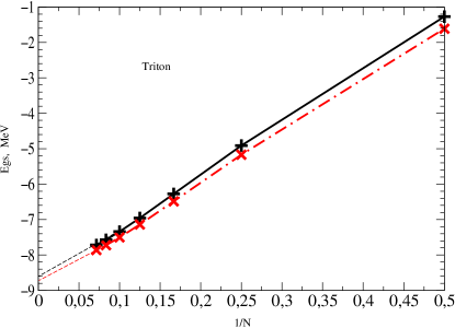
Figure 46: ³H ground state energy obtained in the $N\hbar\omega$ no-core shell model calculation vs $1/N$. $+$ — Version 1 potential model; $\times$ — Version 2 potential model; dashed line — linear extrapolation to the infinite $N\hbar\omega$ model space based on the last two calculated points ; solid and dash-dot lines are to guide the eye.

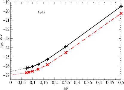
Figure 47: ⁴He ground state energy obtained in the $N\hbar\omega$ no-core shell model calculation vs $1/N$. See Fig. 46 for details.

In Fig. 47 we present the results of the ⁴He ground state energy $E_{\alpha}$ calculations with the same potential models. In the ⁴He case we also obtain very similar results with the Version 1 and the Version 2 potential models. It is interesting that the convergence of the ⁴He ground state energy is better than that of ³H. In this case the curves connecting the $E_{\alpha}$ values deviate from the straight lines. Nevertheless we also perform the linear extrapolations of $E_{\alpha}(1/N)$ to infinite $N$ using the $E_{\alpha}$ values obtained in $12\hbar\omega$ and $14\hbar\omega$ calculations and obtain $E_{\alpha}\approx-26.6$ MeV in the Version 1 potential model and $E_{\alpha}\approx-27.0$ MeV in the Version 2 potential model.

The quality of the linear extrapolation of $E_{\rm g.s.}(1/N)$ may be tested in the deuteron calculations. In the deuteron case, we know the exact result for the infinite $N\hbar\omega$ model space ground state energy $E_{d}=-2.244575$ MeV obtained by the $S$-matrix pole calculation with our potentials. The $E_{d}$ results obtained in the $N\hbar\omega$ model spaces with $N\leq 14$ with the Version 1 and Version 2 $sd$-ISTP, are shown in Fig. 48. It is seen that $E_{d}(1/N)$ seems to be a linear function in the interval $4\leq N\leq 14$. The linear extrapolation results in $E_{d}\approx-2.5$ MeV that differs from the exact energy. Therefore the linear extrapolation results can be regarded only as a rough estimate of the binding energy. However in the ⁴He case we achieved a reasonable convergence and by the linear extrapolation we increase the binding energy by approximately 0.3 MeV only. Therefore our estimate of the ⁴He binding energy seems to be accurate enough.

The differences in convergence rates for the deuteron, ³H and ⁴He can be understood from the fact that $\hbar\omega=40$ MeV is more optimal for the tighter bound ⁴He than for the lesser bound systems.

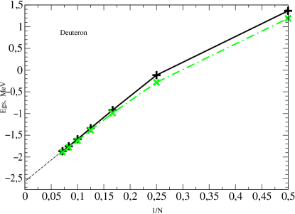
Figure 48: Deuteron ground state energy obtained in the $N\hbar\omega$ no-core shell model calculation vs $1/N$. See Fig. 46 for details.

Table 13: ³H and ⁴He ground state energies (in MeV) obtained in $14\hbar\omega$ no-core shell model calculations and by the linear extrapolation to the infinite $N\hbar\omega$ model space.

Potential	3H		4He
model	$\mbox{\hskip 18.0pt}14\hbar\omega\mbox{\hskip 18.0pt}$	extrapolation	$\mbox{\hskip 18.0pt}14\hbar\omega\mbox{\hskip 18.0pt}$	extrapolation
Version 0	$-9.091$	$9.7$	$-33.223$	$-33.4$
Version 1	$-7.718$	$-8.6$	$-26.241$	$-26.6$
Version 2	$-7.860$	$-8.7$	$-26.734$	$-27.0$
Nature	$-8.48$		$-28.30$

Our results of the ³H and ⁴He ground state energy calculations are summarized in Table 13. We also present in the table the results obtained with the less realistic Version 0 potential model. Both ³H and ⁴He are essentially overbound in this potential model. With both Version 1 and Version 2 potential models we obtain a reasonable description of the ³H and ⁴He bindings. Our ⁴He results are better than the ones obtained (see Ref. alpha-3 ) with any of the realistic meson exchange interactions without allowing for the three-body interactions. In the ³H case, we have underbinding in the $14\hbar\omega$ model space and a small overbinding obtained by the linear extrapolation. Unfortunately, the difference between the $14\hbar\omega$ model space and the linear extrapolation results is rather large. Most probably the ³H ground state energy curve in Fig. 46 will flatten out in larger model spaces. This will shift the extrapolated ground state energy upwards from our current result. Hence the expected ground state energy in the $N\to\infty$ limit lies between the $14\hbar\omega$ and the present linear extrapolation. In other words, our linear extrapolation and $14\hbar\omega$ results are expected to be the lower and upper boundaries for the exact results, respectively. An approximately 0.9 MeV difference between the $14\hbar\omega$ and the linear extrapolation ground state energies in the ³H case indicates the 0.9 MeV uncertainty of our predictions. The ³H ground state energy obtained in Faddeev calculations with CD-Bonn $NN$ potential is $-8.012$ MeV (see alpha-3 ). All the remaining modern realistic meson exchange potentials predict the ³H binding energy to be less than 7.4 MeV alpha-3 . Therefore our ³H binding energy predictions are not worse than those obtained with the realistic meson exchange potentials without allowing for the three-body forces while our ⁴He binding energy predictions are better.

In Fig. 49 we present the spectrum of the lowest excited ⁴He states of each $J^{\pi}$. The description of the excited states energies is reasonable though further from experiment than the ground state. On the other hand, we expect the excited states to be less converged and to drop more in larger model spaces. Of course, a full discussion of the states above breakup must await proper extensions of the theory to the scattering domain.

Figure 49: ⁴He spectrum obtained with Version 2 potential model in the no-core shell model in the $14\hbar\omega$ ($13\hbar\omega$) model space for even (odd) parity states. Dashed line shows the result of the linear extrapolation of the ground state energy to the infinite $N\hbar\omega$ model space. Experimental data are taken from LANL .

V Concluding remarks

We obtained nucleon-nucleon ISTP potentials by means of the $J$-matrix version of the inverse scattering approach. The potentials accurately describe the scattering data. They are in the form of $8\hbar\omega$-truncated matrices in the oscillator basis with $\hbar\omega=40$ MeV. The potential matrices are tridiagonal in the uncoupled partial waves. In the coupled partial waves, the potential matrices have two additional quasi-diagonals in each of the submatrices responsible for the channel coupling. The $sd$-ISTP of this type (Version 0) underestimates the deuteron $d$ state probability and overestimates the deuteron rms radius. We designed two other $sd$-ISTP with two additional matrix elements providing the correct description of the $d$ state probability, one of them (Version 1) overestimates the rms radius by approximately 1.5% while the other one (Version 2) provides the correct description of the deuteron rms radius. All other deuteron observables are reproduced by all $sd$-ISTP versions.

The ISTP potentials are used in the ³H and ⁴He no-core shell model calculations. Both Version 1 and Version 2 ISTP potential models provide very good predictions for the ³H and ⁴He binding energies and a reasonable ⁴He spectrum. With the less realistic Version 0 potential model, we obtain overbound ³H and ⁴He nuclei. We note that there were other attempts to design the $NN$ interaction providing the description of the triton binding energy together with the $NN$ scattering data and the deuteron properties Dole ; Plessas . Our interactions are much simplier and can be directly used in the shell model calculations of heavier nuclei.

Generally our approach is aimed at shell model applications in heavier nuclei. However our potentials are simple enough and can be used directly in other microscopic approaches, e. g. in Faddeev calculations. We hope that our interactions minimize the need for three-body forces. It is known Poly that the three-body force effect can be reproduced in a three-body system by the phase equivalent transformation of the two-body interaction. This phase equivalent transformation can also spoil the description of the deuteron observables, in particular, the deuteron rms radius can be arbitrary changed by phase equivalent transformations RMS . We expect that there exist transformations minimizing the need for three-body force effects, that do not significantly change the nucleon-nucleon interaction. That is, the deuteron properties, the deuteron and scattering wave functions of the transformed $NN$ potential may remain very close to the ones developed here while achieving improved descriptions of other nuclei. In this context, it is worth noting that our approach does not assume either a particular operator structure to the interaction or locality.

From this point of view, the Version 2 ISTP accurately describing the deuteron properties and providing good predictions for the ³H and ⁴He bindings, can be regarded as such an interaction effectively accounting for effects that might otherwise be attributed to three-body forces. Clearly, additional efforts may provide superior NN interactions with less dependence on three-body forces for precision agreement with experiment.

Finally, we suggested a new approach to the construction of the high-quality $NN$ interaction and examined the obtained ISTP $NN$ interaction in three and four nucleon systems by means of the no-core shell model. The ³H and ⁴He binding energies are surprisingly well described. Obviousely it will be very interesting to extend these studies on heavier nuclei, to investigate in detail not only their binding but the spectra of excited states as well. It is also important to investigate more carefully the ISTP description of the two-nucleon system since, for example, we have deferred the discussion of the deuteron quadrupole moment $Q$. We just mention here that the Version 2 ISTP prediction of $Q=0.317$ fm² is not so far from the experimental value of $0.2875\pm 20$ fm² Qdeu . The phase equivalent transformations discussed above make it possible to improve the $Q$ predictions and to examine the effect of such improvement in light nuclear systems. We plan to address this problem in future publications.

This work was supported in part by the State Program “Russian Universities”, by the Russian Foundation of Basic Research grant No 02-02-17316, by US DOE grant No DE-FG-02 87ER40371 and by US NSF grant No PHY-007-1027.

References

• (1) R. Machleidt, F. Sammarruca, and Y. Song, Phys. Rev. C 53, 1483 (1996).
• (2) R. B. Wiringa, V. G. J. Stoks, and R. Schiavilla, Phys. Rev. C 51, 38 (1995).
• (3) V. G. J. Stoks, R. A. M. Klomp, C. P. F. Terheggen, and J. J. de Swart, Phys. Rev. C 49, 2950 (1994).
• (4) S. A. Coon, M. D. Scadron, P. C. McNamee, B. R. Barrett, D. W. E. Blatt, and B. H. J. McKellar, Nucl. Phys. A 317, 242 (1979); J. L. Friar, D. Hüber, and U. van Kolck, Phys. Rev. C 59, 53 (1999); D. Hüber, J. L. Friar, A. Nogga, H. Witala, and U. van Kolck, Few Body Syst. 30, 95 (2001).
• (5) B. S. Pudliner, V. R. Pandharipande, J. Carlson, S. C. Pieper, and R. B. Wiringa, Phys. Rev. C 56, 1720 (1997); R. B. Wiringa, Nucl. Phys. A 631, 70c (1998).
• (6) A. Nogga, H. Kamada, and W. Glöckle, Phys. Rev. Lett. 85, 944 (2000).
• (7) A. Picklesimer, R. A. Rice, and R. Brandenburg, Phys. Rev. Lett. 68, 1484 (1992); Phys. Rev. C 45, 547 (1992); Phys. Rev. C 45, 2045 (1992); Phys. Rev. C 45, 2624 (1992); Phys. Rev. C 46, 1178 (1992).
• (8) S. R. Beane, P. F. Bedaque, W. C. Haxton, D. R. Phillips, M. J. Savage, in: M. Shifman (Ed.), At the Frontier of Particle Physics, Vol. 1, 133 (World Scientific); nucl-th/0008064.
• (9) D. R. Entem, R. Machleidt, Phys. Lett. B 524, 93 (2002).
• (10) H. Kamada, A. Nogga, W. Glöckle, E. Hiyama, M. Kamimura, K. Varga, Y. Suzuki, M. Viviani, A. Kievsky, S. Rosati, J. Carlson, S. C. Pieper, R. B. Wiringa, P. Navrátil, B. R. Barrett, N. Barnea, W. Leidemann, and G. Orlandini, Phys. Rev. C 64, 044001 (2001).
• (11) D. C. Zheng, J. P. Vary, and B. R. Barrett, Phys. Rev. C 50, 2841 (1994); D. C. Zheng, J. P. Vary, B. R. Barrett, W. C. Haxton, and C. L. Song, Phys. Rev. C 52, 2488 (1995).
• (12) P. Navrátil, J. P. Vary, and B. R. Barrett, Phys. Rev. Lett. 84, 5728 (2000); Phys. Rev. C 62, 054311 (2000).
• (13) S. A. Zaytsev, Teoret. Mat. Fiz. 115, 263 (1998) [Theor. Math. Phys. 115, 575 (1998)].
• (14) S. A. Zaytsev, in Proc. XIV Int. Workshop on High Energy Physics and Quantum Field Theory, Moscow 1999) (Ed. B.B.Levchenko and V.I.Savrin), 666 (Moscow, MSU-Press, 2000); Teoret. Mat. Fiz. 121, 424 (1999) [Theor. Math. Phys. 121, 1617 (1999)].
• (15) S. A. Zaitsev and E. I. Kramar J. Phys. G 27, 2037 (2001).
• (16) Yu. A. Lurie and A. M. Shirokov, Izv. Ros. Akad. Nauk, Ser. Fiz. 61, 2121 (1997) [Bull. Rus. Acad. Sci., Phys. Ser. 61, 1665 (1997)].
• (17) Yu. A. Lurie and A. M. Shirokov, to be published in A. D. Alhaidari, E. J. Heller, H. A. Yamani, and M. S. Abdelmonem (eds.), $J$-matrix method and its applications (Nova Science Publishers, Inc.).
• (18) Yu. A. Lurie and A. M. Shirokov, nucl-th/0312028; to be published in Ann. Phys.
• (19) P. Doleschall and I. Berbély, Phys. Rev. C 62, 054004 (2000).
• (20) P. Doleschall, I. Berbély, Z. Papp, and W. Plessas, Phys. Rev. C 67, 064005 (2003).
• (21) S. K. Bogner, T. T. S. Kuo, and A. Schwenk, Phys. Rep. 386, 1 (2003).
• (22) S. Bogner, T. T. S. Kuo, L. Coraggio, A. Covello, and N. Itaco, Phys. Rev. C 65, 051301 (2002).
• (23) H. A. Yamani, L.  Fishman, J. Math. Phys., 16, 410 (1975).
• (24) J. T. Broad and W. P. Reinhardt, Phys. Rev. A 14, 2159 (1976); J. Phys. B 9, 1491 (1976).
• (25) A. M. Shirokov, Yu. F. Smirnov, and L. Ya. Stotland, in Proc. XIIth Europ. Conf. on Few-Body Phys., Uzhgorod, USSR, 1990 (Ed. V. I. Lengyel and M. I. Haysak), 173 (Uzhgorod, 1990).
• (26) Yu. F. Smirnov, L. Ya. Stotland, and A. M. Shirokov, Izv. Akad. Nauk SSSR, Ser. Fiz. 54, No 5, 897 (1990) [Bull. Acad. Sci. USSR, Phys. Ser. 54, No 5, 81 (1990)].
• (27) D. A. Konovalov and I. A. McCarthy, J. Phys. B27, L407 (1994); J. Phys. B27, L741 (1994).
• (28) G. F. Filippov and I. P. Okhrimenko, Yad. Fiz. 32, 932 (1980) [Sov. J. Nucl. Phys. 32, 480 (1980)]; G. F. Filippov, Yad. Fiz. 33, 928 (1981) [Sov. J. Nucl. Phys. 33, 488 (1981)].
• (29) Yu. F. Smirnov and Yu. I. Nechaev, Kinam 4, 445 (1982); Yu. I. Nechaev and Yu. F. Smirnov, Yad. Fiz. 35, 1385 (1982) [Sov. J. Nucl. Phys. 35, 808 (1982)].
• (30) G. F. Filippov, V. S. Vasilevski, and L. L. Chopovski, Fiz. Elem. Chastits At. Yadra 15, 1338 (1984); 16, 349 (1985) [Sov. J. Part. Nucl. 15, 600 (1984); 16, 153 (1985)].
• (31) G. F. Filippov, Rivista Nuovo Cim. 12, 1 (1989).
• (32) V. A. Knyr, A. I. Mazur, and Yu. F. Smirnov, Yad. Fiz. 52, 754 (1990) [Sov. J. Nucl. Phys. 52, 483 (1990)].
• (33) V. A. Knyr, A. I. Mazur, and Yu. F. Smirnov, Yad. Fiz. 54, 1518 (1991) [Sov. J. Nucl. Phys. 54, 927 (1991)].
• (34) Yu. F. Smirnov and A. M. Shirokov, Preprint ITF-88-47R (Kiev, 1988); A. M. Shirokov, Yu. F. Smirnov, and S. A. Zaytsev, in Modern Problems in Quantum Theory (Ed. V. I. Savrin and O. A. Khrustalev), (Moscow, 1998), 184; Teoret. Mat. Fiz. 117, 227 (1998) [Theor. Math. Phys. 117, 1291 (1998)].
• (35) T. Ya. Mikhelashvili, Yu. F. Smirnov, and A. M. Shirokov, Yad. Fiz. 48, 969 (1988) [Sov. J. Nucl. Phys. 48, 617 (1988)]; J. Phys. G 16, 1241 (1990).
• (36) D. E. Lanskoy, Yu. A. Lurie, and A. M. Shirokov, Z. Phys. A 357, 95 (1997).
• (37) J. M. Bang, A. I. Mazur, A. M. Shirokov, Yu. F. Smirnov, and S. A. Zaytsev, Ann. Phys. (NY), 280, 299 (2000).
• (38) M. Abramowitz and I. A. Stegun (eds.), Handbook on Mathematical Functions (Dover, New York, 1972).
• (39) V. V. Babikov, Method of Phase Functions in Quantum Mechanics (Nauka Publishers, Moscow, 1976).
• (40) H. P. Stapp, T. I. Ypsilantis, and N. Metropolis, Phys. Rev. 105, 302 (1957).
• (41) A. I. Baz, Ya. B. Zeldovitch, and A. M. Perelomov, Scattering, Reactions and Decays in Non-relativistic Quantum Mechanics (Nauka Publishers, Moscow, 1971).
• (42) L. D. Blokhintsev, I. Borbely, and É. I. Dolinskii, Sov. J. Part. Nucl. 8, 485 (1977).
• (43) J. J. de Swart, C. P. F. Terheggen, and V. G. J. Stoks, Invited talk by J. J. de Swart at the 3${}^{\mbox{rd}}$ Int. Symp. “Dubna Deuteron 95”, Dubna, Russia, July 4–7, 1995; nucl-th/9509032.
• (44) V. A. Babenko and N. M. Petrov, Yad. Fiz. 66, 1359 (2003) [Phys. At. Nucl. 66, 1319 (2003)].
• (45) LANL T-2 Nucl. Information Service, http://t2.lanl.gov/data/map.html.
• (46) W. N. Polyzou and W. Glöckle, Few-Body Syst. 9, 97 (1990).
• (47) W. N. Polyzou, Phys.Rev. C 58, 91 (1998).
• (48) R. V. Reid, Jr. and M. L. Vaida, Phys. Rev. Lett. 29, 494 (1972).