The three-body problem with short-range forces: renormalized equations and regulator-independent results

Abstract

We discuss effective field theory treatments of the problem of three particles interacting via short-range forces. One case of such a system is neutron-deuteron scattering at low energies. We demonstrate that in attractive channels the renormalization-group evolution of the 1+2 scattering amplitude may be complicated by the presence of eigenvalues greater than unity in the kernel. We also show that these eigenvalues can be removed from the kernel by one subtraction, resulting in an equation which is renormalization-group invariant. A unique solution for 1+2 scattering phase shifts is then obtained. We give an explicit demonstration of our procedure for both the case of three spinless bosons and the case of the doublet channel in nd scattering. After the contribution of the two-body effective range is included in the effective field theory, it gives a good description of the nd doublet phase shifts below deuteron breakup threshold.

I Introduction

For over forty years now the three-nucleon problem has, with considerable success, been used as a testing ground for the nucleon-nucleon interaction. Usually the three-body equations used are based on the Schrödinger equation or its implementation for scattering in the form of the Faddeev Fa61 equations with the two-body interaction being one of finite range. However, discussions of the case in which the range of the interaction is significantly less than the wavelengths of interest, i.e. $kR\ll 1$, also have a long history. There has been renewed interest in this case with the advent of Effective Field Theory (EFT) descriptions of few-nucleon systems at low energy vK99 ; Be00 ; Ph01 . In an EFT treatment of the problem of two- and three-body scattering at energies such that $kR\ll 1$ the two-body scattering problem requires renormalization since the leading-order two-body potential is a three-dimensional delta function.

But in low-energy $NN$ scattering $k$ and $R$ are not the only scales in the problem. The presence of a low-energy bound state in the $NN$ system—the deuteron—means that we must also account for the deuteron binding momentum $\gamma=\sqrt{-m\epsilon_{d}}\sim 1/a$—with $a\gg R$ the unnaturally-large $NN$ scattering length—when we do an EFT analysis of this problem. In technical terms the presence of an enhanced two-body scattering length—or equivalently a near-zero-energy bound state—means that there is a non-trivial fixed point in the renormalization-group evolution of this leading-order potential. As long as this is accounted for, and a power counting built around the scale hierarchy:

$$k\sim\gamma\ll 1/R,$$ (1)

a systematic EFT can be established and renormalized using a variety of regularization schemes We90 ; We91 ; vK97 ; vK98 ; Ka98A ; Ka98B ; Ge98A ; Bi99 . A similar scale hierarchy (and hence a similar EFT) governs the low-energy interactions of Helium-4 atoms Bd99A ; Bd99B ; BH02 . It is also relevant to the physics of Bose-Einstein condensates, if the external magnetic field is adjusted such that the atoms (e.g. ⁸⁵Rb) are near a Feshbach resonance BH01 ; Br02 .

As a first step in extending this EFT to heavier nuclei, the three-nucleon system was considered, and the Faddeev equations for the particular case of a zero-range interaction were solved. It was soon discovered that the leading-order (LO) EFT equation for the quartet (total angular momentum $3/2$) channel yielded a unique solution BvK97 ; Bd98 , while for the doublet (total angular momentum $1/2$) channel the corresponding equation did not yield a unique solution—at least in the absence of three-body forces Bd99A ; Bd99B ; Bd00 . This could be simply understood on the grounds that in the quartet channel the effective interaction between the neutron and the deuteron is repulsive as a result of the Pauli principle, and this ultimately means that the neutron and deuteron do not experience a zero-range interaction. In contrast, in the doublet channel the effective neutron-deuteron interaction is attractive and the full difficulties of the zero-range interaction manifest themselves. These difficulties were first elucidated by Thomas, who pointed out that—if two-body forces alone are employed—the nuclear force must have a finite range if the binding energy of nuclei is to be finite Th35 .

The three-body scattering problem for zero-range interactions considered in the seminal work of Bedaque and collaborators BvK97 ; Bd98 ; Bd99A ; Bd99B ; Bd00 was first considered in research that antedates Faddeev’s landmark 1961 paper: by Skorniakov and Ter-Martirosian STM57 and by Danilov Da61 . These authors found similar difficulties to Bedaque et al., and traced the non-uniqueness to the fact that in the asymptotic region this three-body equation for scattering reduces to a homogeneous equation whose solution can be added to the solution of the inhomogeneous equation with an arbitrary weighting—a point recently reiterated by Blankleider and Gegelia Ge00 ; BlG00 ; BG01 .

In their 1999 papers Bd99A ; Bd99B , Bedaque et al. introduced a three-body force into the leading-order three-body EFT equation, so as to obtain a unique solution for 1+2 phase shifts. They adjusted this force in order to reproduce the experimental 1+2 scattering length. The energy dependence of the 1+2 phase shift was then predicted Bd99A ; Bd99B ; Bd00 . The introduction of this three-body force is unexpected if naive dimensional analysis is used to estimate the size of various effects in the EFT, but it is apparently necessary if the equations are to yield sensible, unique predictions for physical observables. This also accords with the 1995 paper of Adhikhari, Frederico, and Goldman, who pointed out that the divergences in the kernel of the Faddeev equations for a zero-range interaction may necessitate the introduction of a piece of three-body data so that these divergences can be renormalized away Ad95 . (But see Refs. Ge00 ; BlG00 ; BG01 for a conflicting view.)

In an attempt to get some insight into alternative ways to establish a unique solution to the three-body scattering problem at leading order in the effective field theory, we try to bridge the gap between the Faddeev approach—in which the interaction has a finite range—and the EFT formulation of this problem. In Sec. II, we examine the Amado model Am63 for the case of three spinless bosons. Here we look at scattering in which the interaction of an incident particle on a composite system of the other two is considered within the framework of the Lagrangian for the Lee model Le54 ; VAA61 . If three-body forces are neglected then the only difference between this approach and those at LO in the EFT of Refs. We90 ; We91 ; vK97 ; vK98 ; Ka98A ; Ka98B ; Ge98A ; Bi99 is that in the Lee model Lagrangian one may introduce a form factor that plays the role of a cut-off in the theory. In this way we can connect the LO EFT equations (without a three-body force) to those found in the Amado model, by taking the limit as the range of the interaction goes to zero. The resulting equation has a non-compact kernel unless a cutoff is imposed on the momentum integration. We then reproduce and reiterate the results of Refs. STM57 ; Da61 ; Bd99A ; Bd99B , demonstrating that the low-energy solution of the equation changes radically as the cutoff is varied. Using a renormalization-group analysis we trace this unreasonable cutoff dependence to the presence of eigenvalues equal to 1 in the kernel of the integral equation.

In Section III we use a subtraction originally developed by Hammer and Mehen HM00 to remove these eigenvalues. Our analysis of Sec. II then allows us to demonstrate that the subtracted three-body equation is renormalization-group-invariant. The subtraction of Ref. HM00 was employed at a specific energy, and used experimental data from the three-body system to determine the half-off-shell behaviour of the 1+2-amplitude. Here we go further, and show that using low-energy two-body data plus just one piece of experimental data for the three-body system—the 1+2 scattering length—we can predict the low-energy three-body phase shifts. We do this by first solving the subtracted integral equation for the half-off-shell threshold 1+2-amplitude. We then use this result to derive unique predictions for the full off-shell behaviour of the 1+2-threshold-amplitude, and thence for the 1+2-amplitude at any energy. The equations derived in this way are equivalent to those of Bedaque et al., but represent a reformulation of the problem in which only physical, renormalized quantities appear. In consequence the leading-order three-body force of Refs. Bd99A ; Bd99B does not appear in our equations. Our single subtraction ultimately allows us to generate predictions for the energy-dependence of the 1+2 phase shifts at leading order in the EFT without the presence of an explicit three-body force. The subtraction does, though, require data from the three-body system (namely the 1+2 scattering length) before other three-body observables can be predicted.

In Sec. IV we apply the formalism of Secs. II–III to the—conceptually identical but technically more complicated—case of the doublet channel in nd scattering. Here, we compare the numerical solution to our once-subtracted equation with phase-shift data. In Sec. V we consider higher-order corrections to the LO EFT and illustrate that the results from the EFT are in good agreement with the nd data below three-nucleon breakup threshold if the sub-leading (two-body) terms in the EFT expansion are adjusted so as to reproduce the asymptotic S-state normalization of deuterium. The resulting description of the doublet phase shifts is very good up to the deuteron breakup threshold. Finally in Sec. VI we present some concluding remarks regarding the limitations of this method and discuss the convergence and usefulness of the EFT.

II Three-boson scattering at low energy

Consider a system of three bosons at energies so low that the details of their interaction are not probed. Suppose, in addition, that two of the bosons can form a bound state—“the dimer”, with binding energy $-\epsilon_{d}$. In this section we will compute the amplitude for boson-dimer scattering in a low-energy effective theory. This problem has been studied for almost 50 years STM57 , and has recently been revisited in the context of EFT Bd99A ; Bd99B ; Ge00 ; HM01 ; Bd02 . In Sec. II.1 we derive the Faddeev equations for this system, in order to establish the notation used elsewhere in the paper. We then show in Sec. II.2 that this equation is not renormalization-group (RG) invariant, i.e. changing the regularization procedure used in the integral equation alters its physical predictions significantly. In particular, we will demonstrate that this lack of RG invariance is due to the existence of eigenvalues equal to one in the kernel of the integral equation.

II.1 The Amado equations in the limit of zero-range interactions

Consider a field theory of bosons $N$, in which the two-boson bound state (“dimer”) $D$ is included as an explicit degree of freedom. In this model the Lagrangian can be written as Ka97 ; BG00 :

$${\cal L}=N^{\dagger}\left(i\partial_{0}+\frac{\nabla^{2}}{2M}\right)N+D^{\dagger}\,\Delta\,D-g\left[D^{\dagger}NN+DN^{\dagger}N^{\dagger}\right]\ .$$ (2)

Here $\Delta$ is the bare inverse free propagator for the dimer. This is basically the Lee model Le54 for $D\leftrightarrow NN$. Historically, in order to obtain a finite amplitude for boson-dimer scattering, a regularization scheme has been invoked. This can be achieved either through the introduction of a cut-off in all momentum integrals or by including a form factor in the interaction Lagrangian i.e. replacing $g\rightarrow g(p)$, with $p$ is the relative momentum of the two bosons in $D\rightarrow NN$. The Amado model VAA61 ; Am63 entails the second choice for the regularization. As a result the equation for boson-dimer scattering, after partial-wave expansion, takes the form Am63

$$X_{\ell}(q,q^{\prime};E)=2Z_{\ell}(q,q^{\prime};E)+\int\limits_{0}^{\infty}\,dq^{\prime\prime}\,q^{\prime\prime 2}\ 2Z_{\ell}(q,q^{\prime\prime},E)\,\tau\left(E^{(+)}-\frac{q^{\prime\prime 2}}{2\nu}\right)\,X_{\ell}(q^{\prime\prime},q^{\prime};E)\ \ .$$ (3)

with $E^{(+)}=E+i\eta$, $\eta$ a positive infinitesimal. The Born term $Z_{\ell}(q,q^{\prime};E)$ is the amplitude for one-boson exchange, and is given by

$$Z_{\ell}(q,q^{\prime};E)=\frac{\lambda}{2}\,\int\limits_{-1}^{+1}dx\frac{g(K)\,g(Q)}{E-\frac{1}{m}(q^{2}+q^{\prime 2}+\vec{q}\cdot\vec{q\,}^{\prime})}P_{\ell}(x)\ ,$$ (4)

where $x=\hat{q}\cdot\hat{q}^{\prime}$, $P_{\ell}$ is the Legendre function of order $\ell$ and $\lambda=1$ for three identical bosons. In Eq. (4) the relative momenta of the pair in the vertices $D\leftrightarrow NN$ are given by

$$K=\left|\vec{q\,}^{\prime}+\frac{1}{2}\vec{q}\,\right|\quad\mbox{and}\quad Q=\left|\vec{q}+\frac{1}{2}\vec{q\,}^{\prime}\right|\ .$$ (5)

Note that the convention of Lovelace Lo64 for the recoupling coefficient $\lambda$ differs from this by a factor of -1. In fact, as originally shown by Lovelace Lo64 , Eqs. (3) and (4) also govern nd scattering in the $I=\frac{1}{2}$; $S=\frac{3}{2}$ channel, i.e. the quartet, but with $\lambda=-1/2$ (in the convention used in this work). The details of the recoupling algebra for the bosonic, nd quartet, and nd $S=\frac{1}{2}$ channel, are given in Appendix A.

The off-shell two-body $NN$ amplitude for this Lagrangian is of the form

$$t(p,p^{\prime};E)=g(p)\,\tau(E)\,g(p^{\prime})\ ,$$ (6)

where the dressed dimer propagator is given by

$$\tau(E)=\frac{S(E)}{E-\epsilon_{d}}\ ,$$ (7)

with $\epsilon_{d}$ the energy of the dimer bound-state ($\epsilon_{d}<0$). The function $S(E)$ is:

$$S(E)=\left[\int\limits_{0}^{\infty}\,\frac{dp\,p^{2}\,g^{2}(p)}{(E-\frac{p^{2}}{m})(\epsilon_{d}-\frac{p^{2}}{m})}\right]^{-1}\ ,$$ (8)

and the residue of the $NN$ propagator at the dimer pole is then clearly $S(\epsilon_{d})$.

At this stage the regularization function $g(p)$ is present in the dressing of the dimer propagator $\tau(E)$, and also in the one-nucleon exchange amplitude $Z_{\ell}(q,q^{\prime};E)$. In writing Eqs. (7) and (8), we have imposed the renormalization condition that the binding energy of the dimer takes its physical value. After this renormalization is performed the subtracted integral in Eq. (8) is finite and the cut-off function $g(p)$ can be taken to be one. In that limit

$$\tau(E)=\frac{S(E)}{E-\epsilon_{d}}=\frac{2}{\pi m^{2}}\ \frac{\gamma+\sqrt{-mE}}{E-\epsilon_{d}},\ .$$ (9)

with $\gamma\equiv\sqrt{-m\epsilon_{d}}$. The form of the two-body amplitude (6) is—in the limit $g\rightarrow 1$—exactly that obtained at leading order in an effective field theory with short-range interactions alone We90 ; We91 ; vK97 ; vK98 ; Ka98A ; Ka98B ; Ge98A ; Bi99 .

This allows us to write the integral equation for 1+2 scattering in the limit $g(p)\rightarrow 1$ as

$$X_{\ell}(q,q^{\prime};E)=2Z_{\ell}(q,q^{\prime};E)+\int\limits_{0}^{\infty}dq^{\prime\prime}\,q^{\prime\prime 2}\,2Z_{\ell}(q,q^{\prime\prime};E)\,\frac{S\left(E^{(+)}-\frac{3q^{\prime\prime 2}}{4m}\right)}{E^{(+)}-\frac{3q^{\prime\prime 2}}{4m}-\epsilon_{d}}\,X_{\ell}(q^{\prime\prime},q^{\prime};E)\ ,$$ (10)

where, for $\ell=0$, the Born term $2Z_{0}(q,q^{\prime};E)$ is given by

$$2Z_{0}(q,q^{\prime};E)\equiv{\cal Z}(q,q^{\prime};E)=-\lambda\,\frac{m}{qq^{\prime}}\ln\left[\frac{q^{2}+q^{\prime 2}+qq^{\prime}-mE}{q^{2}+q^{\prime 2}-qq^{\prime}-mE}\right]\ ,$$ (11)

and

$$S\left(E-\frac{3q^{2}}{4m}\right)\equiv S(E;q)=\frac{2}{\pi m^{2}}\ \left[\,\gamma+\sqrt{\frac{3}{4}q^{2}-mE}\,\right]\ .$$ (12)

Here, we have included the factor of 2 resulting from the symmetrization for identical particles in Eq. (3) in the definition of ${\cal Z}$. These equations are identical to those employed in the EFT of Refs. Bd99B ; Bd02 , although with different normalization for the amplitude $X_{\ell}$. The relationship between our conventions and those of Refs. Bd99B ; Bd02 is elucidated further in Appendix B.

In the above analysis we considered the integral equation for the scattering amplitude or $T$-matrix. At any finite $k$ the kernel of the integral equation has a pole, coming from the dimer propagator (see Eq. (10)). Furthermore, above the breakup threshold, the Born amplitude ${\cal Z}$ develops moving logarithmic singularities that need to be dealt with when this equation is solved numerically, for instance by performing a contour rotation that avoids these singularities. In this work we restrict the analysis to energies below the dimer-breakup threshold, and so the logarithmic $NNN$ cut is not an issue. In this energy domain a reformulation of Eq. (10) that eliminates the $D$ pole is useful.

The reformulation involves writing the $DN$ propagator:

$$\frac{1}{E^{(+)}-\epsilon_{d}-\frac{3q^{\prime\prime 2}}{4m}}={\cal P}\frac{1}{E-\epsilon_{d}-\frac{3q^{\prime\prime 2}}{4m}}-i\pi\delta\left(E-\epsilon_{d}-\frac{3q^{\prime\prime 2}}{4m}\right)$$ (13)

We can then calculate the amplitude $X_{0}$ of Eq. (10) by first calculating the boson-dimer S-wave $K$-matrix using the integral equation:

$$K(q,q^{\prime};E)={\cal Z}(q,q^{\prime};E)+{\cal P}\int\limits_{0}^{\infty}dq^{\prime\prime}\,q^{\prime\prime 2}\,{\cal Z}(q,q^{\prime\prime};E)\,\frac{S(E;q^{\prime\prime})}{E-\epsilon_{d}-\frac{3q^{\prime\prime 2}}{4m}}\,K(q^{\prime\prime},q^{\prime};E)\ .$$ (14)

Below the three-body breakup threshold $K$ is a real symmetric matrix, and this equation is free of singularities. It is therefore numerically advantageous to solve this equation rather than Eq. (10), and this is the approach we have used in generating our numerical results.

The relationship of the phase shifts to the on-shell K-matrix $K(k,k;E)$, is provided by first employing the relation:

$$X_{0}(q,q^{\prime};E)=K(q,q^{\prime};E)-\frac{2im\pi k}{3}K(q,k;E)S(E;k)X_{0}(k,q^{\prime};E).$$ (15)

Then, to determine the S-wave on-shell scattering amplitude and therefore the S-wave phase shift, we need to multiply the result from Eq. (15) by the residue of the dimer propagator, i.e. define

$$T_{0}(q,q^{\prime};E)=S^{1/2}(q,E)\,X_{0}(q,q^{\prime};E)\,S^{1/2}(q^{\prime},E)\ .$$ (16)

The boson-dimer S-wave scattering phase shifts are then related to the amplitude $T_{0}$ at the on-shell point by:

$$T_{0}(k,k;E)=-\frac{3}{2m\pi k}\,e^{i\delta}\sin\delta\ ,$$ (17)

where the on-shell momentum $k$ is defined by the relation

$$E-\frac{3k^{2}}{4m}=\epsilon_{d}.$$ (18)

Using the relationships (15) and (17) we find that:

$$K(k,k;E)=-\frac{3m}{8\gamma k}\tan\delta.$$ (19)

Since we will be using the boson-dimer scattering length to renormalize our integral equation, we are particularly interested in the case $E=\epsilon_{d}$ in Eq. (19). Using the boson-dimer effective-range expansion:

$$k\cot\delta=-\frac{1}{a_{3}}+\frac{1}{2}r_{3}k^{2}+\cdots,$$ (20)

with $a_{3}$ and $r_{3}$ being respectively, the boson-dimer scattering length and effective range, we find:

$$K(0,0;\epsilon_{d})=\frac{3ma_{3}}{8\gamma}.$$ (21)

II.2 Renormalization-group invariance

Now consider the convergence properties of the integrals in the equation (14). If $q$ and $q^{\prime\prime}$ are both large then ${\cal Z}$ behaves as $1/{qq^{\prime\prime}}$, while $S$ scales as $q^{\prime\prime}$. Therefore the convergence of the integral in (14) depends on the behaviour of $X(q^{\prime\prime},k;E)$ at large $q^{\prime\prime}$. Perturbation theory suggests that at large $q^{\prime\prime}$

$$K(q^{\prime\prime},k;E)\sim{\cal Z}(q^{\prime\prime},k;E)\sim 1/q^{\prime\prime 2},$$ (22)

and thus the integral equation will be well-behaved without the need to impose any sort of regulator on the integral. However, this conclusion is erroneous.

In fact, the kernel of (14) has infinitely many eigenvalues of order unity, as pointed out in Ref. Da61 , and discussed in detail by Amado and Noble AN72 . The argument of Amado and Noble may be heuristically paraphrased as follows. Calculating the trace of the kernel of Eq. (14) at $E=\epsilon_{d}$ we obtain:

$${\rm tr(kernel)}=\frac{8\lambda}{3\pi}\int\limits_{0}^{\infty}\frac{dq^{\prime\prime}}{q^{\prime\prime}}\ln\left(\frac{3q^{\prime\prime 2}+\gamma^{2}}{q^{\prime\prime 2}+\gamma^{2}}\right)\left(\frac{\gamma}{q^{\prime\prime}}+\sqrt{\frac{3}{4}+\left(\frac{\gamma}{q^{\prime\prime}}\right)^{2}}\right),$$ (23)

an integral which diverges, and does so logarithmically. Since the corrections proportional to $\left(\frac{\gamma}{q^{\prime\prime}}\right)^{2}$ do not affect the ultraviolet behaviour of this integral, if a cutoff $\Lambda$ is imposed we have

$$\rm{tr(kernel)}\rightarrow\frac{4\ln 3}{\sqrt{3}\pi}\ln(\Lambda)$$ (24)

as $\Lambda\rightarrow\infty$. Simple power-counting arguments demonstrate that the trace of all (positive-integer) powers of the kernel contain a logarithmic divergence too. Since it is also the case that the largest eigenvalue of the kernel is finite the only way we can have

$$\rm{tr(kernel^{n})}\sim\ln\left(\frac{\Lambda}{\gamma}\right)$$ (25)

for all $n\geq 1$ is if the number of eigenvalues larger than one grows logarithmically with $\Lambda$—a result in accord with the analysis of Danilov Da61 and Efimov Ef70 ; Ef71 .

As we will discuss in more detail below, the presence of these order-one eigenvalues means that the perturbation theory estimate of $K$’s large-momentum behaviour is incorrect. Consequently a cutoff must be imposed on the integral in (14), as otherwise the integrals diverge. Once this is done the integral equation yields a unique solution for a fixed value of $\Lambda$. In this work we impose a sharp cutoff $\Lambda$, but choosing other, smoother cutoff functions does not alter the essence of the following argument.

This regularization results in an equation:

$$K_{\Lambda}(q,q^{\prime};E)={\cal Z}(q,q^{\prime};E)+{\cal P}\int\limits_{0}^{\Lambda}dq^{\prime\prime}\,q^{\prime\prime 2}\,{\cal Z}(q,q^{\prime\prime};E)\,\frac{S(E-\frac{3q^{\prime\prime 2}}{4m})}{E-\epsilon_{d}-\frac{3q^{\prime\prime 2}}{4m}}\,K_{\Lambda}(q^{\prime\prime},q^{\prime};E)\ ,$$ (26)

where the presence of the cutoff has made $K$ implicitly dependent on $\Lambda$. If the predictions of the theory are to be sensible we must have

$$\Lambda\frac{dK_{\Lambda}(q,q^{\prime};E)}{d\Lambda}\sim 0\quad\mbox{for}\quad q,q^{\prime}\ll\Lambda.$$ (27)

In other words, the low-energy predictions of our boson-dimer scattering calculation should not be affected by the imposition of a cutoff at a momentum scale far above the ones that are physically of interest. The demand (27) represents the renormalization group (RG) for this problem.

Applying $\Lambda\frac{d}{d\Lambda}$ to both sides of Eq. (26) we find that:

$$\Lambda\frac{dK_{\Lambda}}{d\Lambda}(q,q^{\prime};E) = \Lambda^{3}{\cal Z}(q,\Lambda;E)\frac{S(E;\Lambda)}{E-\epsilon_{d}-\frac{3\Lambda^{2}}{4m}}K_{\Lambda}(\Lambda,q^{\prime};E)$$ (28)

$$+ {\cal P}\int\limits_{0}^{\Lambda}dq^{\prime\prime}\,q^{\prime\prime 2}\,{\cal Z}(q,q^{\prime\prime};E)\,\frac{S(E;q^{\prime\prime})}{E-\epsilon_{d}-\frac{3q^{\prime\prime 2}}{4m}}\,\Lambda\frac{dK_{\Lambda}}{d\Lambda}(q^{\prime\prime},q^{\prime};E).$$

For $q,k\ll\Lambda$

$${\cal Z}(q,\Lambda;E)\sim\frac{1}{\Lambda^{2}};\qquad S(E;\Lambda)\sim\Lambda,$$ (29)

and, using the fact (which can be justified a postieri) that $K(\Lambda,q^{\prime};E)\sim\frac{1}{\Lambda}$ for $\Lambda\gg q^{\prime}$ the first term on the right hand side drops out of the integral equation (28) leaving:

$$\Lambda\frac{dK_{\Lambda}}{d\Lambda}(q,k;E)={\cal P}\int\limits_{0}^{\Lambda}dq^{\prime\prime}\,q^{\prime\prime 2}{\cal Z}(q,q^{\prime\prime};E)\,\frac{S(E;q^{\prime\prime})}{E-\epsilon_{d}-\frac{3q^{\prime\prime 2}}{4m}}\,\Lambda\frac{dK_{\Lambda}}{d\Lambda}(q^{\prime\prime},k;E).$$ (30)

At this point it is tempting to argue that since Eq. (30) has a trivial solution, it follows that $K_{\Lambda}$ is RG invariant (up to terms of $O(1/\Lambda)$). Such a conclusion is hasty, however. Non-trivial solutions to Eq. (30) exist if the kernel has an eigenvalue of one. In fact, the presence of eigenfunctions of this kernel corresponding to eigenvalue one has been proven rigorously in the asymptotic regime $q\gg\gamma,k$ by Danilov Da61 and by Amado and Noble AN72 . Here we repeat the analysis of Bedaque et al. Bd99A ; Bd99B , which demonstrates the presence of such an eigenvector. The impact of this “zero-mode” on the spectrum of the kernel has also been discussed by Gegelia and Blankleider BlG00 ; BG01 and by Bedaque et al. Bd02 .

Consider $E=\epsilon_{d}$, i.e. scattering at the threshold for the $ND$ channel. Further, consider off-shell momenta $q$ such that $\gamma\ll q\ll\Lambda$. In this limit we may neglect terms proportional to $\gamma$ in $S(E;q)$ and ${\cal Z}(q,q^{\prime\prime};E)$, and so the integrand becomes scale invariant:

$$\Lambda\frac{dK_{\Lambda}}{d\Lambda}(q,0;\epsilon_{d})=\frac{4\lambda}{\sqrt{3}\pi}\frac{1}{q}\int\limits_{0}^{\infty}dq^{\prime\prime}\,\ln\left[\frac{q^{2}+q^{\prime\prime 2}+qq^{\prime\prime}}{q^{2}+q^{\prime\prime 2}-qq^{\prime\prime}}\right]\Lambda\frac{dK_{\Lambda}}{d\Lambda}(q^{\prime\prime},0;\epsilon_{d}).$$ (31)

Inspired by the absence of any physical scale under the integral we seek a power-law solution:

$$\Lambda\frac{dK_{\Lambda}}{d\Lambda}(q,0;\epsilon_{d})\sim q^{s-1}$$ (32)

As shown in Refs. Da61 ; Bd99A ; Bd99B , such a solution exists provided that $s$ obeys the transcendental equation:

$$\frac{8\lambda}{\sqrt{3}s}\frac{\sin\left(\frac{\pi s}{6}\right)}{\cos\left(\frac{\pi s}{2}\right)}=1.$$ (33)

If $\lambda=1$ this equation has complex roots $s=\pm is_{0}$ with $s_{0}=1.0062$. Thus in this case the RG equation has non-trivial solutions, which, provided $\Lambda\gg q\gg\gamma$, are of the form:

$$f(q)=\frac{1}{q}C\cos\left(s_{0}\ln\left(\frac{q}{\Lambda}\right)+\delta\right).$$ (34)

Note that Eq. (31) also governs $K(q,0;\epsilon_{d})$, at least for $\Lambda\gg q\gg\gamma$, and so a similar analysis applied to $K$ itself justifies the scaling $K(q,0;\epsilon_{d})\sim 1/q$ Bd99A ; Bd99B .

For finite $\Lambda$ we can examine the eigenvalue spectrum of the common kernel of Eqs. (26) and (30). Doing this at $E=\epsilon_{d}\Leftrightarrow k=0$ and $\lambda=1$ for a variety of cutoffs yields the results shown in Fig. 1. As the cutoff increases there are more and more eigenvalues larger than one, with a new eigenvalue of one appearing each time the cutoff is increased by a factor of $e^{\pi/s_{0}}=22.7$. This corresponds to an increasing number of bound states of the boson-dimer system described by Eq. (26), with the number of bound states growing as AN72 :

$$N=\frac{1.0062}{\pi}\ln\left(\frac{\Lambda}{\gamma}\right).$$ (35)

This accumulation of zero-energy bound states in a system with zero-range interactions was first pointed out by Efimov Ef70 ; Ef71 (see also Ref. AN72 ).

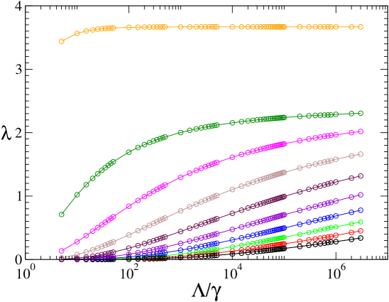
Figure 1: The largest ten eigenvalues of the kernel of Eq. (30), for the case $\lambda=1$, and a range of cutoffs.

The presence of these eigenvalues which cross one as the cutoff is increased manifests itself as non-trivial cutoff dependence when Eq. (26) is solved. Some results found by solving this equation for the half-off-shell amplitude (again at zero energy) are displayed in Fig. 2. Here $K(q,0;\epsilon_{d})\sim 1/q$, and so we have chosen to present results for the quantity:

$$a(q,k)\equiv-\frac{2\pi mS(E;q)}{3}X_{0}(q,k;E).$$ (36)

This also aids comparison with the results of Ref. Bd99B , with which we are in complete agreement. The renormalization-group argument of this section ties the large changes in the low-momentum amplitude seen in Fig. 2 to the spectrum of the kernel of Eq. (26), via the concomitant strong-RG evolution of $K_{\Lambda}$ at low momentum.

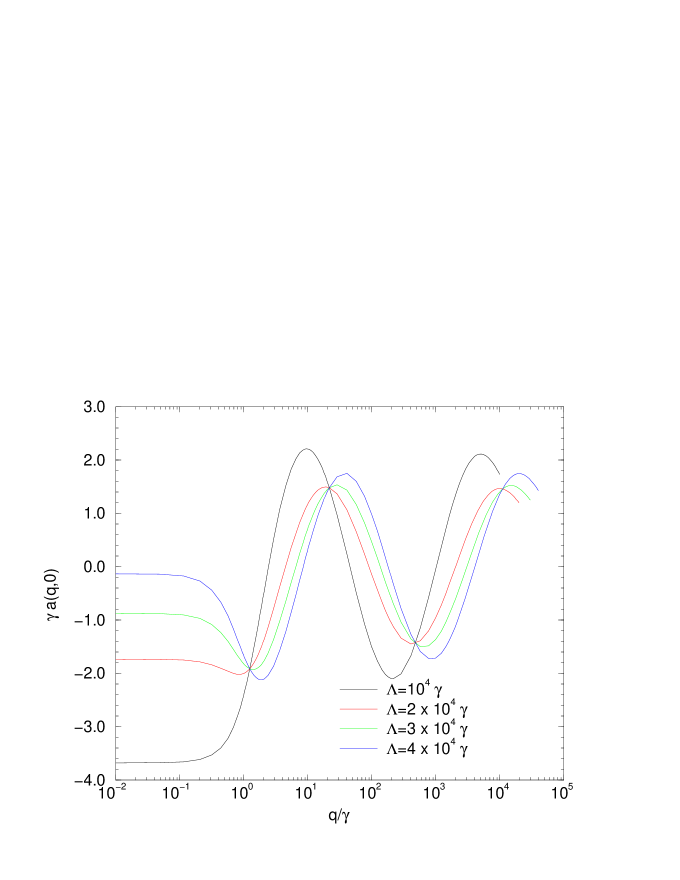
Figure 2: Results for $a(q,0)$, as defined in Eq. (36) when various different cutoffs are imposed on the integral equation (14).

Note that in contrast to the case $\lambda=1$, if $\lambda=-\frac{1}{2}$ then the kernel of Eq. (26) has no eigenvalues larger than one, and so the renormalization-group evolution of the K-matrix is smooth in that case. This means that as $\Lambda\rightarrow\infty$ there is no cutoff-dependence in the predictions for phase shifts—as was seen to be the case numerically Ref. BvK97 ; Bd98 where calculations of nd scattering in the quartet channel were performed in the EFT. (See also Ref. Bd02 .) The coupling at which the large-$\Lambda$ RG evolution becomes non-trivial is the value at which Eq. (33) first develops complex roots. This is Da61 :

$$\lambda_{c}=\frac{3\sqrt{3}}{4\pi}.$$ (37)

III The method of subtraction

Thus, as it stands, if $\lambda>\lambda_{c}$, Eq. (14) needs additional renormalization before it can yield RG-invariant predictions. The solution proposed in Ref. Bd99A ; Bd99B was to add a counterterm to cancel the cutoff-dependence observed in Fig. 2. The three-body force introduced to renormalize the integral equation is not naively of the same order as the terms in the EFT Lagrangian (2), but the analysis of Ref. Bd99A ; Bd99B , which has been recast in the previous section, shows that it is necessary for renormalization. The naive dimensional analysis estimate of the size of three-body forces is trumped by the presence of the shallow bound state in the two-body system, which is ultimately what leads to the Efimov spectrum shown in Fig. 1. Of course, as with any counterterm which removes cutoff-dependence in a quantum field theory, a piece of data is required to fix the value of the counterterm at a particular scale. In Ref. Bd99A ; Bd99B the boson-dimer scattering length $a_{3}$, was chosen for this purpose.

More recently Blankleider and Gegelia BlG00 ; BG01 have avoided introducing a three-body force in the leading-order three-body EFT equation by examining the solution of the homogeneous equation and subtracting the oscillatory behavior. However, in their work no predictions for phase shifts were actually made. A subtraction technique for the three-body problem with zero-range forces was also suggested by Adhikari, Frederico, and Goldman Ad95 . This technique was implemented in another integral equation with a non-compact kernel, that describing unregulated one-pion-exchange between two nucleons FTT99 . However, the subtraction in Ref. FTT99 is performed at large negative energy, and involves demanding equivalence of the full and Born amplitudes at these energies.

In this work we suggest an approach which is equivalent to that used in Ref. Bd99A ; Bd99B , but is formulated in an alternative fashion. Our procedure involves a subtraction of the on-shell amplitude at some—arbitrarily chosen but low—energy. The subtracted equation has a unique solution, which is, up to corrections suppressed by $(p/\Lambda)^{2}$, RG-invariant.

III.1 Subtraction at threshold

Let us first consider the subtraction method applied to the integral equation for the half-off-shell $1+2$ three boson threshold amplitude. We use information on the boson-dimer scattering length to fix the on-shell amplitude at the threshold.

Consider Eq. (14) for the half off-shell amplitude at $E=\epsilon_{d}$, i.e.

$$K(q,0;\epsilon_{d})={\cal Z}(q,0;\epsilon_{d})-\frac{4m}{3}\int\limits_{0}^{\Lambda}dq^{\prime\prime}\,{\cal Z}(q,q^{\prime\prime};\epsilon_{d})\,S(\epsilon_{d};q^{\prime\prime})\,K(q^{\prime\prime},0;\epsilon_{d})\ .$$ (38)

On the other hand, the on-shell amplitude at threshold should obey:

$$K(0,0;\epsilon_{d})=\frac{3ma_{3}}{8\gamma}={\cal Z}(0,0;\epsilon_{d})-\frac{4m}{3}\int\limits_{0}^{\Lambda}dq^{\prime\prime}\,{\cal Z}(0,q^{\prime\prime};\epsilon_{d})\ S(\epsilon_{d};q^{\prime\prime})\ K(q^{\prime\prime},0;\epsilon_{d})\ .$$ (39)

If we now subtract Eq. (39) from Eq. (38), we get an integral equation for the half-off-shell amplitude for which the input is the boson-dimer scattering length $a_{3}$, in addition to the two-body data, which in lowest order is just the binding energy of the dimer. This equation is

$$K(q,0;\epsilon_{d})=\frac{3ma_{3}}{8\gamma}+\Delta{\cal Z}(q,0;\epsilon_{d})-\frac{4m}{3}\int\limits_{0}^{\Lambda}dq^{\prime\prime}\,\Delta{\cal Z}(q,q^{\prime\prime};\epsilon_{d})\,S(q^{\prime\prime};\epsilon_{d})\,K(q^{\prime\prime},0;\epsilon_{d}),\$$ (40)

where

$$\Delta{\cal Z}(q,q^{\prime};E)\equiv{\cal Z}(q,q^{\prime};E)-{\cal Z}(0,q^{\prime};E)\ .$$ (41)

This equation (albeit in different notation) was first derived by Hammer and Mehen HM00 .

In eq. (40) we have an integral equation in which the kernel goes to zero faster as $q^{\prime\prime}\rightarrow\infty$ than does that of the original integral equation. As a result we hope for a unique solution to Eq. (40), even if Eq. (38) does not admit a unique solution. To establish this we need to prove that the amplitude $K(q,0;\epsilon_{d})$ is independent of the cut-off $\Lambda$, i.e. the solution is renormalization group invariant. Here we proceed as above, and differentiate the subtracted equation (40) with respect to the cut-off $\Lambda$, to obtain

$$\Lambda\frac{\partial K(q,0;\epsilon_{d})}{\partial\Lambda} = -\frac{4m}{3}\,\Lambda\,\Delta{\cal Z}(q,\Lambda;\epsilon_{d})\,S(\Lambda;\epsilon_{d})\,K(\Lambda,0;\epsilon_{d})$$ (42)

$$-\frac{4m}{3}\int\limits_{0}^{\Lambda}dq^{\prime\prime}\,\Delta{\cal Z}(q,q^{\prime\prime};\epsilon_{d})\,S(q^{\prime\prime};\epsilon_{d})\,\Lambda\frac{\partial K(q^{\prime\prime},0;\epsilon_{d})}{\partial\Lambda}\ .$$

Once again, we consider $\gamma\ll q\ll\Lambda$, and in this regime:

$$\Delta{\cal Z}(q,\Lambda;\epsilon_{d})\sim\frac{q^{2}}{\Lambda^{4}};\qquad S(\epsilon_{d};\Lambda)\sim\Lambda;$$ (43)

the inhomogeneous term in Eq. (42) goes to zero as $q^{2}/\Lambda^{3}$ for large $\Lambda$. Therefore, once again, in the limit $\Lambda\rightarrow\infty$ Eq. (42) is a homogeneous equation of the form

$$\Lambda\frac{\partial K(q,0;\epsilon_{d})}{\partial\Lambda}=-\frac{4m}{3}\int\limits_{0}^{\Lambda}dq^{\prime\prime}\,\Delta{\cal Z}(q,q^{\prime\prime};\epsilon_{d})\,S(q^{\prime\prime};\epsilon_{d})\,\Lambda\frac{\partial K(q^{\prime\prime},0;\epsilon_{d})}{\partial\Lambda}\ .$$ (44)

It is now easy to show that the kernel of Eq. (44) is negative definite. Thus, no matter how large we make $\Lambda$ no eigenvalues of one can appear. This is demonstrated numerically in Fig. 3 where we plot the eigenvalues of the subtracted integral equation’s kernel as a function of $\Lambda/\gamma$. (Here we have chosen $a_{3}\gamma=-2$.) For the subtracted case, the kernel of the homogeneous equation, Eq. (44), has no eigenvalue close to one, thus there are no solutions to Eq. (44) and that Eq. (27) is satisfied, i.e. the amplitude $K(q,0,\epsilon_{d})$ is independent of the cut-off $\Lambda$—up to corrections of $O(\frac{q^{2}}{\Lambda^{3}})$ and $O(\frac{\gamma^{2}}{\Lambda^{3}})$.

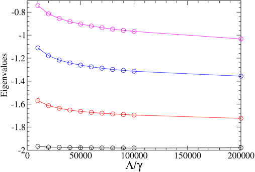
Figure 3: Eigenvalues of the kernel of the subtracted integral equation (14) for various different cutoffs, for the case $a_{3}\gamma=-2$.

In Fig. 4, we present, for several values of the cut-off $\Lambda$, the half-off-shell $K$-matrix at threshold $K(q,0;\epsilon_{d})$ that results from the subtracted equation. It is clear from the results that the solution of the subtracted equation is completely independent of $\Lambda$ in the regime $q\ll\Lambda$, as anticipated from the RG argument above. In fact the cutoff can be numerically taken to infinity without any difficulty at all.

Note that in the asymptotic regime $\gamma\ll q\ll\Lambda$ the subtracted equation (40) still has solutions $K(q,0;\epsilon_{d})$ of the form (34). These solutions ensure equality of the first piece of the integral in (40) with the left-hand side of that equation, $K(q,0;\epsilon_{d})$. However, in contrast to the situation of the previous subsection, the solution of the subtracted equation in this asymptotic regime is not scale invariant. It must still obey Eq. (39), since those pieces of Eq. (40) do not disappear when a solution of the form (34) is inserted. Thus—unlike the case of Eq. (14)—the asymptotic limit of (40) is enough to determine the asymptotic phase $\delta$: $\delta$ is fixed such that (39) is obeyed.

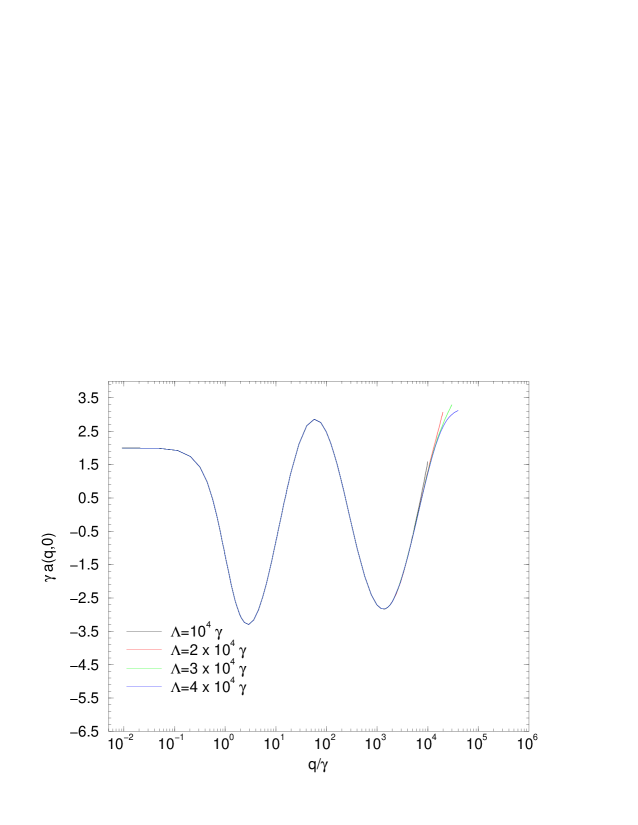
Figure 4: Results for $a(q,0)$ (see Eq. (36) for definition) when various different cutoffs are imposed on the subtracted integral equation (14). Here $a_{3}\gamma$ was chosen to be -2.

Thus our subtracted equation at threshold yields unique results for the half-off-shell amplitude without the need for an explicit three-body force. It also confirms that one piece of three-body experimental data is needed to properly renormalize the integral equation for the three-boson problem in the zero-range limit.

III.2 The subtracted equation at any energy

The above analysis was restricted to the amplitude at threshold and established that the solution of the subtracted equation is unique. The question now is: can we get the amplitude at any energy without any further subtractions? In other words: can we use the half-off-shell amplitude at one energy and the original equation (26) to obtain a RG-well-behaved $K_{\Lambda}$ at all energies?

To answer this, we need to write the on-shell amplitude at energy $E$ in terms of the solution of the half off-shell amplitude at threshold. We do this in two stages. Rewriting Eq. (40) as

$$K(q,0;\epsilon_{d})=K(0,0;\epsilon_{d})+\Delta[{\cal Z}](q,0;\epsilon_{d})-\frac{4m}{3}\int\limits_{0}^{\Lambda}dq^{\prime\prime}\,\Delta[{\cal Z}](q,q^{\prime\prime};\epsilon_{d})\,S(q^{\prime\prime};\epsilon_{d})\,K(q^{\prime\prime},0;\epsilon_{d})\ ,$$ (45)

and having determined the half-off-shell amplitude at threshold, we first need to determine the full-off-shell amplitude at threshold, i.e. $K(q,q^{\prime};\epsilon_{d})$. Before subtraction $K(q,q^{\prime};\epsilon_{d})$ satisfies the equation:

$$K(q,q^{\prime};\epsilon_{d})={\cal Z}(q,q^{\prime};\epsilon_{d})-\frac{4m}{3}\int\limits_{0}^{\Lambda}dq^{\prime\prime}\,{\cal Z}(q,q^{\prime\prime};\epsilon_{d})\,S(q^{\prime\prime};\epsilon_{d})\,K(q^{\prime\prime},q^{\prime};\epsilon_{d})\ ,$$ (46)

which has the original badly-behaved kernel of Eq. (26). So, again we need to perform a subtractive renormalization.

Since ${\cal Z}(q,q^{\prime};E)={\cal Z}(q^{\prime},q;E)$, we have that $K(0,q;\epsilon_{d})=K(q,0;\epsilon_{d})$. But we know that $K(0,q^{\prime};E)$, also satisfies the equation

$$K(0,q^{\prime};\epsilon_{d})={\cal Z}(0,q^{\prime};\epsilon_{d})-\frac{4m}{3}\int\limits_{0}^{\Lambda}dq^{\prime\prime}{\cal Z}(0,q^{\prime\prime};\epsilon_{d})\,S(q^{\prime\prime};\epsilon_{d})\,K(q^{\prime\prime},q;\epsilon_{d})\ .$$ (47)

We can now subtract this equation from the equation for the full off-shell amplitude—Eq. (46)—to get:

$$K(q,q^{\prime};\epsilon_{d})=K(0,q^{\prime};\epsilon_{d})+\Delta[{\cal Z}](q,q^{\prime};\epsilon_{d})-\frac{4m}{3}\int\limits_{0}^{\Lambda}dq^{\prime\prime}\,\Delta[{\cal Z}](q,q^{\prime\prime};\epsilon_{d})\,S(q^{\prime\prime};\epsilon_{d})\,K(q^{\prime\prime},q^{\prime};\epsilon_{d})\ .$$ (48)

This equation has the same kernel as Eq. (45), and given that we have already determined $K(0,q^{\prime};\epsilon_{d})=K(q^{\prime},0;\epsilon_{d})$, we can now determine the full off-shell amplitude at the elastic threshold. Numerical solution indeed confirms that the solution of Eq. (48) is cutoff independent, and that the limit $\Lambda\rightarrow\infty$ can be taken. The resulting $K(q,q^{\prime};\epsilon_{d})$ is also, by construction, real and symmetric. In this way we have established that the full, off-shell, amplitude at threshold can be determined with one subtraction, and therefore, given $a_{3}$, we know the amplitude $K(\epsilon_{d})=X(\epsilon_{d})$.

To derive the renormalized equation at any energy $E$ for the amplitude $X(E)$, we need to write the boson-dimer equation at the energy $E$, i.e.

$$X(E)={\cal Z}(E)+{\cal Z}(E)\,\tau(E)\,X(E)\ ,$$ (49)

and the threshold equation

$$X(\epsilon_{d})={\cal Z}(\epsilon_{d})+{\cal Z}(\epsilon_{d})\,\tau(\epsilon_{d})\,X(\epsilon_{d})\ .$$ (50)

(Note that we will manipulate the equations for $X$, but the same manipulations can equally well be done with $K$.) These two equations can be written as:

$${\cal Z}^{-1}(E) = X^{-1}(E)+\tau(E)$$ (51)

$${\cal Z}^{-1}(\epsilon_{d}) = X^{-1}(\epsilon_{d})+\tau(\epsilon_{d})\ .$$ (52)

We now subtract Eq. (52) from Eq. (51) with the result that

$$\delta[\tau] \equiv \tau(E)-\tau(\epsilon_{d})=\left[{\cal Z}^{-1}(E)-{\cal Z}^{-1}(\epsilon_{d})\right]-\left[X^{-1}(E)-X^{-1}(\epsilon_{d})\right]$$ (53)

$$= {\cal Z}^{-1}(\epsilon_{d})\left[{\cal Z}(\epsilon_{d})-{\cal Z}(E)\right]{\cal Z}^{-1}(E)-X^{-1}(\epsilon_{d})\left[X(\epsilon_{d})-X(E)\right]X^{-1}(E)\ .$$

Multiply this equation from the left by $X(\epsilon_{d})$ and from the right by $X(E)$, we get

$$X(E) = X(\epsilon_{d})+[1+X(\epsilon_{d})\,\tau(\epsilon_{d})]\delta[{\cal Z}]+X(\epsilon_{d})\delta[\tau]\,X(E)$$ (54)

$$+[1+X(\epsilon_{d})\,\tau(\epsilon_{d})]\,\delta[{\cal Z}]\,\tau(E)\,X(E)\ ,$$

where

$$\delta[{\cal Z}]={\cal Z}(E)-{\cal Z}(\epsilon_{d})\ .$$ (55)

All integrals in the above equation have sufficient ultraviolet decay to be finite, with the possible exception of $X(\epsilon_{d})\,\tau(\epsilon_{d})\,\delta[{\cal Z}]\,\tau(E)\,X(E)$ which is a double integral.

We now can write the above operator equation as an integral equation for the amplitude at a given energy $E$ in terms of the fully-off-shell amplitude at threshold, $X(q^{\prime},q;\epsilon_{d})$, as input:

$$X(q,k;E)=X(q,k;\epsilon_{d})+B(q,k;E)+\int\limits_{0}^{\Lambda}\,dq^{\prime}\,q^{\prime 2}\ Y(q,q^{\prime};E)\ X(q^{\prime},k;E)\ ,$$ (56)

Where the second inhomogeneous term is

$$B(q,k;E)=\delta[{\cal Z}](q,k;E)+\int\limits_{0}^{\Lambda}\,dq^{\prime\prime}\,q^{\prime\prime 2}\ X(q,q^{\prime\prime};\epsilon_{d})\ \tau(\epsilon_{d};q^{\prime\prime})\ \delta[{\cal Z}](q^{\prime\prime},k;E)\ ,$$ (57)

with

$$\delta[{\cal Z}](q,k;E)={\cal Z}(q,k;E)-{\cal Z}(q,k;\epsilon_{d})\ ,$$ (58)

and $\tau(E;q)\equiv\tau(E-\frac{3q^{2}}{4m})$. Meanwhile the kernel of the integral equation is given by

$$Y(q,q^{\prime};E) = X(q,q^{\prime};\epsilon_{d})\ \delta[\tau](E;q^{\prime})+\delta[{\cal Z}](q,q^{\prime};E)\ \tau(E;q^{\prime})$$ (59)

$$\qquad+\int\limits_{0}^{\Lambda}\,dq^{\prime\prime}\,q^{\prime\prime 2}\ X(q,q^{\prime\prime};\epsilon_{d})\ \tau(\epsilon_{d};q^{\prime\prime})\ \delta[{\cal Z}](q^{\prime\prime},q^{\prime};E)\ \tau(E;q^{\prime})$$

$$= X(q,q^{\prime};\epsilon_{d})\ \delta[\tau](E;q^{\prime})+B(q,q^{\prime};E)\ \tau(E;q)\ ,$$

with

$$\delta[\tau](E;q)=\tau(E;q)-\tau(\epsilon_{d};q)\ .$$ (60)

In this way we can determine the half off-shell and from it, the on-shell amplitude, at any energy given the on-shell amplitude at one energy where the subtractive renormalization is done. Note that if $\delta{\cal Z}=0$, i.e. the “potential” for the scattering equation is energy-independent, then $B=0$ and $Y(E)=X(\epsilon_{d})\delta[\tau](E)$.

To test our procedure, we have calculated the boson-dimer phase shifts, for the case $a_{3}\gamma=1.56$. This value was chosen since models of the helium-4 dimer suggest a ratio of three-body and two-body scattering lengths of this size Bd99A ; Bd99B . In Figure 5 we plot $k\cot(\delta)$ against $k$ (in units of $\gamma$) for five different cutoffs. Our results agree exactly with those reported in Ref. Bd99A ; Bd99B . In contrast to the figure presented in Ref. Bd99B , we see absolutely no cutoff dependence whatsoever in our results. No explicit three-body force is required to perform this renormalization.

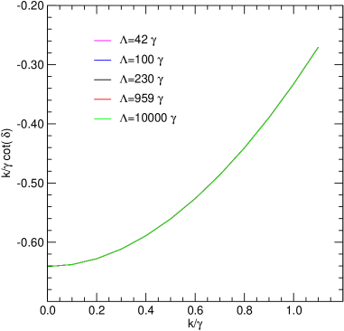
Figure 5: Phase shifts for boson-dimer scattering in the case $a_{3}\gamma=1.56$, for a number of different cutoffs. The curves are completely indistinguishable.

IV Neutron-deuteron scattering in the doublet channel

In the last section we formally developed the procedure for calculating the amplitude for 1+2-scattering in the three-boson system at any energy, having renormalized the equation at threshold using the boson-dimer scattering length as input experimental data. The final results were identical for different cut-offs $\Lambda$. So far in our analysis we considered the three-boson problem in order to avoid the additional complication of coupled-channel integral equations. However, in order to establish the ability of the once-subtracted equations in EFT to reproduce experimental nd scattering data, we need to introduce the spin and isospin dependence of the nd scattering problem. The tensor interaction in the $NN$ system is only manifest at higher order in the EFT without explicit pions, and in this Section we will restrict our analysis to lowest order in this EFT, known as EFT$(\not\!\pi)$, thus here we need only include the ¹S₀ and ³S₁ nucleon-nucleon channels. Since the nucleon-nucleon interaction in the ¹S₀ has anti-bound state, we can still write a dimer-like propagator in this channel, but now the subtraction point must be the energy of the anti-bound state. As a result we write the quasi-deuteron propagator as

$$\tau_{\alpha}(E)=\frac{S_{\alpha}(E)}{E-\epsilon_{\alpha}}\quad\mbox{with}\quad\alpha=s,t\ ,$$ (61)

where $s$ and $t$ stand for the spin singlet and spin triplet nucleon-nucleon channels respectively, and:

$$\epsilon_{s}=-\frac{1}{ma_{s}^{2}}; a_{s}^{-1}=-7.88~{}{\rm MeV},$$ (62)

$$\epsilon_{d}=-\frac{\gamma^{2}}{m}; \gamma=45.71~{}{\rm MeV}.$$ (63)

The nd equations in the doublet channel are now a set of two coupled integral equations in which the initial channel has the deuteron in the triplet ($t$), while intermediate states can have either a singlet ($s$) or triplet ($t$) $NN$ pair with a spectator nucleon, all coupled to spin and iso-spin one half. These equations take the form

$$K_{tt}(q,q^{\prime};E) = {\cal Z}_{tt}(q,q^{\prime};E)+{\cal P}\int\limits_{0}^{\Lambda}\ dq^{\prime\prime}\,q^{\prime\prime 2}\ {\cal Z}_{tt}(q,q^{\prime\prime};E)\,\tau_{t}\left(E-\frac{q^{\prime\prime 2}}{2\nu}\right)\ K_{tt}(q^{\prime\prime},q^{\prime};E)$$ (64)

$$\qquad+{\cal P}\int\limits_{0}^{\Lambda}\ dq^{\prime\prime}\,q^{\prime\prime 2}\ {\cal Z}_{ts}(q,q^{\prime\prime};E)\,\tau_{s}\left(E-\frac{q^{\prime\prime 2}}{2\nu}\right)\ K_{st}(q^{\prime\prime},q^{\prime};E)$$

$$K_{st}(q,q^{\prime};E) = {\cal Z}_{st}(q,q^{\prime};E)+{\cal P}\int\limits_{0}^{\Lambda}\ dq^{\prime\prime}\,q^{\prime\prime 2}\ {\cal Z}_{st}(q,q^{\prime\prime};E)\,\tau_{t}\left(E-\frac{q^{\prime\prime 2}}{2\nu}\right)\ K_{tt}(q^{\prime\prime},q^{\prime};E)$$ (65)

$$\qquad+{\cal P}\int\limits_{0}^{\Lambda}\ dq^{\prime\prime}\,q^{\prime\prime 2}\ {\cal Z}_{ss}(q,q^{\prime\prime};E)\,\tau_{s}\left(E-\frac{q^{\prime\prime 2}}{2\nu}\right)\ K_{st}(q^{\prime\prime},q^{\prime};E)\ .$$

where $\nu=\frac{2}{3}m$ is the reduced mass for the nd system, and the Born amplitude ${\cal Z}_{\alpha\beta}$ is given by

$${\cal Z}_{\alpha\beta}(q,q^{\prime};E)=-\lambda_{\alpha\beta}\ \frac{m}{qq^{\prime}}\ \ln\left\{\frac{q^{2}+q^{\prime 2}+qq^{\prime}-mE}{q^{2}+q^{\prime 2}-qq^{\prime}-mE}\right\}\ ,$$ (66)

with the spin iso-spin factor matrix ${\bf\lambda}$ given by:

$${\bf\lambda}=\frac{1}{4}\left(\begin{array}[]{cc}1&-3\\ -3&1\end{array}\right)\ .$$ (67)

It is not immediately apparent that the kernel of the coupled integral equations (64) and (65) has the same problems as that of (26). By taking linear combinations of (64) and (65) and looking in the asymptotic region we can perform an analysis akin to that used for Eq. (26) Bd00 . This shows that one subtraction is required to render the system (64)–(65) well-behaved. Otherwise this kernel too, has eigenvalues which cross one as $\Lambda$ is increased, and the RG-evolution of $K_{tt}$ at low momenta will not be smooth.

In this case the $K_{tt}(0,0;\epsilon_{d})$, as given by Eq. (21), with $a_{3}$ the doublet scattering length, is chosen for the subtraction. Experimentally Di71 :

$$a_{3}=0.65\pm 0.04~{}{\rm fm}.$$ (68)

We adopt the central value for $a_{3}$.

After the subtraction is performed the equations for the half-off-shell threshold amplitude become:

$$K_{tt}(q,0;\epsilon_{d}) = K_{tt}(0,0;\epsilon_{d})+\Delta{\cal Z}_{tt}(q,0;\epsilon_{d})$$ (69)

$$\qquad+\int\limits_{0}^{\Lambda}\ dq^{\prime\prime}\,q^{\prime\prime 2}\ \Delta{\cal Z}_{tt}(q,q^{\prime\prime};E)\,\tau_{t}\left(\epsilon_{d}-\frac{q^{\prime\prime 2}}{2\nu}\right)\ K_{tt}(q^{\prime\prime},0;\epsilon_{d})$$

$$\qquad+\int\limits_{0}^{\Lambda}\ dq^{\prime\prime}\,q^{\prime\prime 2}\ \Delta{\cal Z}_{ts}(q,q^{\prime\prime};\epsilon_{d})\,\tau_{s}\left(\epsilon_{d}-\frac{q^{\prime\prime 2}}{2\nu}\right)\ K_{st}(q^{\prime\prime},0;\epsilon_{d})$$

$$K_{st}(q,0;\epsilon_{d}) = K_{tt}(0,0;\epsilon_{d})+[{\cal Z}_{st}(q,0;\epsilon_{d})-{\cal Z}_{tt}(0,0;\epsilon_{d})]$$ (70)

$$\qquad+\int\limits_{0}^{\Lambda}\ dq^{\prime\prime}\,q^{\prime\prime 2}\ [{\cal Z}_{st}(q,q^{\prime\prime};\epsilon_{d})-{\cal Z}_{tt}(0,q^{\prime\prime};\epsilon_{d})]\,\tau_{t}\left(\epsilon_{d}-\frac{q^{\prime\prime 2}}{2\nu}\right)\ K_{tt}(q^{\prime\prime},0;\epsilon_{d})$$

$$\qquad+\int\limits_{0}^{\Lambda}\ dq^{\prime\prime}\,q^{\prime\prime 2}\ [{\cal Z}_{ss}(q,q^{\prime\prime};\epsilon_{d})-{\cal Z}_{ts}(0,q^{\prime\prime};\epsilon_{d})]\,\tau_{s}\left(\epsilon_{d}-\frac{q^{\prime\prime 2}}{2\nu}\right)\ K_{st}(q^{\prime\prime},0;\epsilon_{d})\ .$$

Once these equations have been solved for $K_{tt}(q,0;\epsilon_{d})$ and $K_{st}(q,0;\epsilon_{d})$ we can demand:

$$K_{tt}(q,0;\epsilon_{d})=K_{tt}(0,q;\epsilon_{d});\qquad K_{ts}(0,q;\epsilon_{d})=K_{st}(q,0;\epsilon_{d}),$$ (71)

and so arrive at two sets of two coupled equations apiece. These four equations determine the fully-off-shell threshold nd scattering amplitude. The first pair is:

$$K_{tt}(q,q^{\prime};\epsilon_{d}) = K_{tt}(0,q^{\prime};\epsilon_{d})+\Delta{\cal Z}_{tt}(q,q^{\prime};\epsilon_{d})$$ (72)

$$\qquad+\int\limits_{0}^{\Lambda}\ dq^{\prime\prime}\,q^{\prime\prime 2}\ \Delta{\cal Z}_{tt}(q,q^{\prime\prime};\epsilon_{d})\,\tau_{t}\left(\epsilon_{d}-\frac{q^{\prime\prime 2}}{2\nu}\right)\ K_{tt}(q^{\prime\prime},q^{\prime};\epsilon_{d})$$

$$\qquad+\int\limits_{0}^{\Lambda}\ dq^{\prime\prime}\,q^{\prime\prime 2}\ \Delta{\cal Z}_{ts}(q,q^{\prime\prime};\epsilon_{d})\,\tau_{s}\left(\epsilon_{d}-\frac{q^{\prime\prime 2}}{2\nu}\right)\ K_{st}(q^{\prime\prime},q^{\prime};\epsilon_{d})$$

$$K_{st}(q,q^{\prime};\epsilon_{d}) = K_{tt}(0,q^{\prime};\epsilon_{d})+[{\cal Z}_{st}(q,q^{\prime};\epsilon_{d})-{\cal Z}_{tt}(0,q^{\prime};\epsilon_{d})]$$

$$\qquad+\int\limits_{0}^{\Lambda}\ dq^{\prime\prime}\,q^{\prime\prime 2}\ [{\cal Z}_{st}(q,q^{\prime\prime};\epsilon_{d})-{\cal Z}_{tt}(0,q^{\prime\prime};\epsilon_{d})]\,\tau_{t}\left(\epsilon_{d}-\frac{q^{\prime\prime 2}}{2\nu}\right)\ K_{tt}(q^{\prime\prime},q^{\prime};\epsilon_{d})$$

$$\qquad+\int\limits_{0}^{\Lambda}\ dq^{\prime\prime}\,q^{\prime\prime 2}\ [{\cal Z}_{ss}(q,q^{\prime\prime};\epsilon_{d})-{\cal Z}_{ts}(0,q^{\prime\prime};\epsilon_{d})]\,\tau_{s}\left(\epsilon_{d}-\frac{q^{\prime\prime 2}}{2\nu}\right)\ K_{st}(q^{\prime\prime},q^{\prime};\epsilon_{d})\ ,$$

which have exactly the same kernel as (69) and (70), but different driving terms.

The second set of subtracted equations describes the (unphysical) amplitudes $K_{ts}$ and $K_{ss}$ at threshold. The unsubtracted versions of these equations are given by a simple extension of Eqs. (64) and (65). After subtraction the equations are:

$$K_{ts}(q,q^{\prime};\epsilon_{d}) = K_{ts}(0,q^{\prime};\epsilon_{d})+\Delta{\cal Z}_{ts}(q,q^{\prime};\epsilon_{d})$$ (74)

$$\qquad+\int\limits_{0}^{\Lambda}dq^{\prime\prime}\,q^{\prime\prime 2}\Delta{\cal Z}_{tt}(q,q^{\prime\prime};\epsilon_{d})\tau_{t}\left(\epsilon_{d}-\frac{q^{\prime\prime 2}}{2\nu}\right)K_{ts}(q^{\prime\prime},q^{\prime};\epsilon_{d})$$

$$\qquad+\int\limits_{0}^{\Lambda}dq^{\prime\prime}\,q^{\prime\prime 2}\Delta{\cal Z}_{ts}(q,q^{\prime\prime};\epsilon_{d})\tau_{s}\left(\epsilon_{d}-\frac{q^{\prime\prime 2}}{2\nu}\right)K_{ss}(q^{\prime\prime},q^{\prime};\epsilon_{d})$$

$$K_{ss}(q,q^{\prime};\epsilon_{d}) = K_{ts}(0,q^{\prime};\epsilon_{d})+{\cal Z}_{ss}(q,q^{\prime};\epsilon_{d})-{\cal Z}_{ts}(0,q^{\prime};\epsilon_{d})$$

$$\qquad+\int\limits_{0}^{\Lambda}dq^{\prime\prime}\,q^{\prime\prime 2}[{\cal Z}_{st}(q,q^{\prime\prime};\epsilon_{d})-{\cal Z}_{tt}(0,q^{\prime\prime};\epsilon_{d})]\tau_{t}\left(\epsilon_{d}-\frac{q^{\prime\prime 2}}{2\nu}\right)K_{ts}(q^{\prime\prime},q^{\prime};\epsilon_{d})$$

$$\qquad+\int\limits_{0}^{\Lambda}dq^{\prime\prime}\,q^{\prime\prime 2}[{\cal Z}_{ss}(q,q^{\prime\prime};\epsilon_{d})-{\cal Z}_{ts}(q,q^{\prime\prime};\epsilon_{d})]\tau_{s}\left(\epsilon_{d}-\frac{q^{\prime\prime 2}}{2\nu}\right)K_{ss}(q^{\prime\prime},q^{\prime};\epsilon_{d}).$$

Note that imposing (71) to perform the subtraction on the set of four original integral equations (written in matrix form in Appendix B) leads to a symmetric result for the 2 $\times$ 2 matrix form of the threshold amplitude.

Now we write the original, unsubtracted, equations in operator form, as:

$${\bf K}(E)={\bf{\cal Z}}(E)+{\bf{\cal Z}}(E)\,{\bf\tau}(E)\,{\bf K}(E),$$ (76)

with ${\bf K}$ the 2 $\times$ 2 matrix:

$${\bf K}\equiv\left(\begin{array}[]{cc}K_{tt}&K_{ts}\\ K_{st}&K_{ss}\end{array}\right);$$ (77)

$${\bf\tau}(E;q^{\prime\prime})\equiv\left(\begin{array}[]{cc}\tau_{t}\left(E-\frac{q^{\prime\prime 2}}{2\nu}\right)&0\\ 0&\tau_{s}\left(E-\frac{q^{\prime\prime 2}}{2\nu}\right)\end{array}\right).$$ (78)

and ${\bf{\cal Z}}$ the 2 $\times$ 2 matrix defined by Eq. (66).

We can then perform the formal manipulations that lead to Eqs. (56)–(60), except that now all quantities are 2 $\times$ 2 matrices in channel space, and thus the final integral equation to be solved is, in matrix form, but with the momentum-dependence made explicit:

$${\bf X}(q,k;E)={\bf X}(q,k;\epsilon_{d})+{\bf B}(q,k;E)+\int\limits_{0}^{\Lambda}dq^{\prime\prime}\,q^{\prime\prime 2}\,{\bf Y}(q,q^{\prime\prime};E)\,{\bf X}(q^{\prime\prime},k;E),$$ (79)

with:

$${\bf B}(E) = \delta[{\bf{\cal Z}}]+{\bf X}(\epsilon_{d}){\bf\tau}(\epsilon_{d})\delta[{\bf{\cal Z}}]$$ (80)

$${\bf Y}(E) = {\bf X}(\epsilon_{d})\delta[\tau]+{\bf B}(E){\bf\tau}(E),$$ (81)

where the meaning of the energy-difference operator $\delta$ is exactly as in the boson case of the previous section.

Applying these equations to scattering in the nd doublet channel below the nnp breakup threshold yields the phase shifts shown in Fig. 6. At almost all energies shown these agree with the leading-order results published in Ref. HM01 at the 1% level. Once again, there is no cutoff dependence, once the doublet scattering length is used to subtractively renormalize the equations. Also shown are the results of a phase-shift analysis vOS67 , and the results of a calculation using the AV18 $NN$ and UIX $NNN$ potential Ki96 .

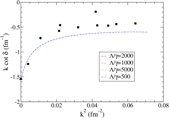
Figure 6: Phase shifts for neutron-deuteron scattering at low energies, at leading order in the nucleon-nucleon EFT without explicit pions, for a variety of different cutoffs. The curves for different cutoffs are indistinguishable. The triangle is the central value of the scattering length measurement of Ref. Di71 . The circles are the results of the van Oers-Seagrave phase-shift analysis vOS67 , and the squares represent a recent calculation of these phase shifts by Kievsky et al. Ki96 .

V The nd doublet channel beyond leading order

In this section we discuss calculations of nd doublet scattering which go beyond the leading-order calculation of the previous section. That computation employed the Lagrangian (2), extended to the $NN$ system. This Lagrangian is equivalent to BG00 :

$${\cal L}^{(0)}={\cal L}=N^{\dagger}\left(i\partial_{0}+\frac{\nabla^{2}}{2M}\right)N-\sum_{\alpha=s,t}{}^{\not\pi}C_{0,-1}^{(\alpha)}(N^{T}P^{\alpha}_{a}N)^{\dagger}(N^{T}P^{\alpha}_{a}N)$$ (82)

with $P^{\alpha}_{a}$ the spin-isopsin projector which restricts the interactions to the ³S₁ or ¹S₀ channel, as appropriate:

$$P^{s}_{a}=\frac{1}{\sqrt{8}}\sigma_{2}\,\tau_{2}\tau_{a};\qquad P^{t}_{a}=\frac{1}{\sqrt{8}}\sigma_{2}\sigma_{a}\,\tau_{2},$$ (83)

and ${}^{\not\pi}C_{0,-1}^{(\alpha)}$ is the leading-order contact interaction in these channels. The subscript _0,-1 on this coefficient indicates that it appears in front of an interaction which has no derivatives, but that it scales as $Q^{-1}$, with the enhancement over its naive dimensional analsysis scaling being due to the presence of the unnaturally-large scattering lengths in the two-body system vK97 ; vK98 ; Ka98A ; Ka98B ; Bi99 .

The higher-order calculation we report on in this section requires the insertion of higher-derivative four-nucleon operators. The analysis of Refs. vK98 ; Ka98A ; Ka98B ; Bi99 indicates that the first additional piece of the EFT Lagrangian which must be considered is Be00 :

$${\cal L}^{(1)}=-\sum_{\alpha=s,t}{}^{\not\pi}C_{0,0}^{(\alpha)}(N^{T}P^{\alpha}_{a}N)^{\dagger}(N^{T}P^{\alpha}_{a}N)-{}^{\not\pi}C_{2}^{(\alpha)}\frac{1}{2}\left[(N^{T}P_{a}^{\alpha}N)^{\dagger}(N^{T}{\cal O}^{2,\alpha}_{a}N)+{\rm h.c.}\right]$$ (84)

and the Hermitian, two-derivative three-component, operator ${\cal O}^{2,\alpha}$ is defined by:

$${\cal O}^{2,\alpha}_{a}=-\frac{1}{4}\left[P^{\alpha}_{a}\overrightarrow{\bf\nabla}^{2}+\overleftarrow{\bf\nabla}^{2}P^{\alpha}_{a}-2\overleftarrow{\bf\nabla}P^{\alpha}_{a}\overrightarrow{\bf\nabla}\right].$$ (85)

Here the effect of the two-derivative operators on the $NN$ amplitude is suppressed by one power of the small parameter $\gamma R$ ($R/a_{s}$ in the ¹S₀ case) relative to the leading-order EFT amplitude. Also appearing in ${\cal L}^{(1)}$ is a small correction to $C_{0}$, denoted by ${}^{\not\pi}C_{0,0}$: “small” because ${}^{\not\pi}C_{0,0}$ is down by $\gamma R$ relative to ${}^{\not\pi}C_{0,-1}$ vK98 ; Ka98A ; Ka98B ; Bi99 .

Thus the effects of the terms in ${\cal L}^{(1)}$ on the $NN$ amplitude can be calculated in perturbation theory. ${}^{\not\pi}C_{2}^{({}^{3}S_{1})}$ can then be chosen so as to reproduce the asymptotic S-state normalization of deuterium Ph99 , and ${}^{\not\pi}C_{0,0}^{({}^{3}S_{1})}$ adjusted in such a way that double-pole term which would otherwise appear in the $NN$ EFT amplitude is removed. This produces a next-to-leading order (NLO) ³S₁ $NN$ amplitude Be00 :

$$T(p)=\frac{2}{\pi m}\left[\frac{Z_{t}}{\gamma+ip}-\frac{Z_{t}-1}{2\gamma}\right],$$ (86)

with $p=\sqrt{ME}$, and where $Z_{t}$ is the residue of the ³S₁ T-matrix at the deuteron pole $p=i\gamma$. This amplitude is easily seen to be a re-expanded version of the effective-range-theory ³S₁ amplitude:

$$T(p)=\frac{2}{\pi m}\frac{1}{\gamma-\frac{1}{2}\rho_{t}(p^{2}+\gamma^{2})+ip},$$ (87)

where $\rho_{t}$ is the $NN$ ³S₁ effective range, which is of order the range of the $NN$ interaction: $\rho_{t}\sim R$. The re-expansion is thus in the small parameters $\rho_{t}\gamma$ and $\rho_{t}p$, but with $\gamma$ treated as being of the same size as $p$. By making such an identification we determine that:

$$Z_{t}=\frac{1}{1-\gamma\rho_{t}}.$$ (88)

$Z_{t}$ is also related to the asymptotic S-state normalization of deuterium, $A_{S}$ PC99 ; Ph99 :

$$A_{S}^{2}=2\gamma Z_{t}.$$ (89)

Using the Nijmegen PSA value for $A_{S}$, $A_{S}=0.8845~{}{\rm fm}^{-1/2}$ St93 ; deS95 , we obtain:

$$Z_{t}=1.686,$$ (90)

which agrees with the result obtained from Eq. (88) to three significant figures.

To summarize, the coefficients in the NLO EFT Lagrangian may be chosen such that the amplitude in the ³S₁ channel has a deuteron pole with the experimental binding energy and the “experimental” asymptotic S-state normalization. Also present in the NLO $NN$ ³S₁ amplitude is a constant piece, which is proportional to $\rho_{t}$. Here we wish only to assess the impact of higher-order terms on the nd phase shifts, and thus, we will perform a partial NLO calculation of the nd phase shifts below breakup threshold, dropping the non-pole term in Eq. (85). Work on complete higher-order calculations within our subtractive framework is in progress, and these numerical studies, as well as prior results by other authors HM01 ; Bd02 indicate that including the constant term of Eq. (85) has little effect on nd phase shifts below nd breakup threshold .

Similar results follow for the NLO ¹S₀ amplitude, and there:

$$Z_{s}=\frac{1}{1-r_{s}/a_{s}},$$ (91)

$r_{s}=2.73$ fm St93 being the effective range in this channel. This results in much smaller NLO corrections from this channel, since $r_{s}/a_{s}$ is only of order 10%.

Thus, to perform our (partial) next-to-leading-order calculation for nd scattering the only changes to the amplitude which are necessary are the multiplication of $\tau_{t}$ and $\tau_{s}$ by factors $Z_{t}$ and $Z_{s}$. The subtractive procedure developed above is not affected by the inclusion of these factors: the only changes necessary in the above equations are the replacements

$$S_{t}\rightarrow S_{t}Z_{t};\qquad S_{s}\rightarrow S_{s}Z_{s}.$$ (92)

Making these replacements we obtain the results shown in Fig. 7. Once again the result is cutoff independent. It agrees remarkably well with the sophisticated potential-model calculation of Kievsky et al. Ki96 . The agreement with the single-energy phase-shift analysis of van Oers and Seagrave vOS67 is not as pleasing, but it is clear that modern potential-model calculations do not agree with these older doublet phase shifts either.

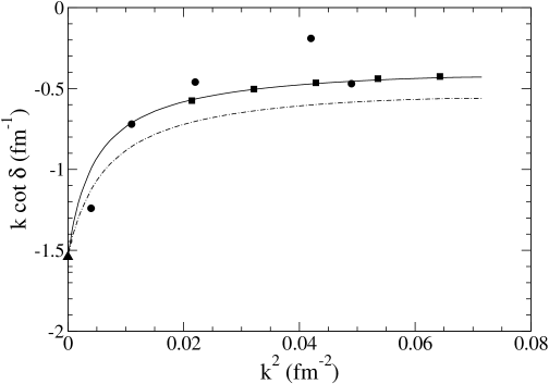
Figure 7: Phase shifts for neutron-deuteron scattering at low energies, at leading order (dash-dotted) and next-to-leading order (solid) in the nucleon-nucleon EFT without explicit pions. The curves for different cutoffs are indistinguishable. Data are as described in Fig. 6.

These results are a (partial) NLO calculation of the nd phase shifts below breakup. They differ from those of Refs. HM01 ; Bd02 since in those works the authors chose to adjust the NLO coefficients in the EFT Lagrangian to reproduce $\rho_{t}$ exactly, and so only obtained $Z_{t}$ (or equivalently $A_{S}$) approximately. The difference between this “$\rho$-parameterization” and our “$Z$-parameterization” is a higher-order effect, and the magnitude of the discrepancy between the results of Fig. 7 and those of Refs. HM01 ; Bd02 is consistent with an effect of order $(\rho_{t}\gamma)^{2}$, i.e. two orders beyond leading. Comparison of our numerical results with those of Ref. Bd02 indicates that if we adopt the $\rho$-parameterization the agreement is better than 1% Gr03 .

VI Conclusions

The integral equation which describes 1+2-scattering in the effective field theory with short-range interactions alone does not yield an RG-invariant low-energy amplitude. By performing an RG-analysis of the integral equation for this process we traced this poor RG behaviour to the presence of eigenvalues of order one in the kernel of the integral equation. One subtraction removes these eigenvalues from the spectrum of the kernel and renders it negative definite (at threshold). Imposing Hermiticity and employing a series of resolvent identities we can use this single subtraction at the 1+2-threshold to generate predictions for phase shifts at finite energies. Note that although here we have only computed phase shifts below 1+2-breakup threshold our subtractive technique is easily extended to include energies above the three-body threshold. The only complication is the technical one of dealing with the logarithmic branch cuts that appear in the kernel of the integral equation at this energy.

The equations we have developed are equivalent to the equations of Bedaque et al. Bd99A ; Bd99B , and may be obtained from those equations by algebraic manipulations. The distinguishing feature of our formulation is that the equations are subtractively renormalized, i.e. only physical quantities appear in them, and any regulator can be employed. This would appear to make this formulation especially useful for higher-order computations in the nd system. It also provides particular emphasis to the point that – as in the case with all bare parameters in field-theoretic Lagrangian – the three-body force which appears in the equations of Bedaque et al. is not an observable.

Thus one piece of three-body experimental data is needed in order to renormalize the three-body equations for zero-range forces. For this piece of data we choose the 1+2 scattering length. Its value can be incorporated into the EFT description of the three-body system either via a counterterm, as in Refs. Bd99A ; Bd99B ; Bd00 or, as done here, by a subtraction of the badly-behaved integral equation. The renormalization of the equation after the inclusion of this single piece of three-body data provides a simple, model-independent, explanation for well-known features of the three-nucleon system such as the Phillips line Ph68 . It also facilitates the systematization of predictions made by Efimov for such systems Ef81 ; Ef85 ; Ef91 ; Ef93 .

Finally, we performed a partial treatment of next-to-leading order corrections to the doublet nd phase shifts in the EFT. We found that adopting coefficients in the NLO EFT($\not\!\pi$) Lagrangian that give the correct deuteron binding energy and asymptotic S-state normalization results in excellent reproduction of potential-model $S=\frac{1}{2}$ nd phase shifts below deuteron breakup threshold. Our results suggest that—to a very good level of approximation— these nd phase shifts are determined by four numbers from the two-body system, $\epsilon_{d}$, $A_{S}$, and the ¹S₀ scattering length and effective range, together with the crucial one piece of data from the three-body system: the nd doublet scattering length.

Appendix A Spin-isospin factors for the Amado equation

In this appendix we derive the spin-isospin factors for the Amado model for: (i) three bosons; (ii) nd quartet; (iii)  nd doublet. In the latter two cases we restrict our analysis to S-waves only.

The Amado equation can be written in operator form as

$$X=2Z+2Z\,\tau\ X$$

where

$$Z_{\alpha\beta}=(1-\delta_{\alpha\beta})\langle g_{\alpha}|G_{0}(E)|g_{\beta}\rangle$$

with $G_{0}(E)=(E-H_{0})^{-1}$. Note: This differs from Lovelace Lo64 by $(-1)$ due to a different definition of $G_{0}$.

This $Z_{\alpha\beta}$ can be written after partial wave expansion as

$$Z_{\alpha\beta}=\lambda_{\alpha\beta}\ \frac{1}{2}\,\int\limits_{-1}^{+1}dx\frac{g_{\alpha}(p_{\alpha})\ g_{\beta}(p_{\beta})}{E-\frac{1}{m}(q_{\alpha}^{2}+q_{\beta}^{2}+q_{\alpha}q_{\beta}x)}\ P_{\ell}(x)$$

where $\lambda_{\alpha\beta}$ is the product of a spin factor $\Lambda^{S}_{\alpha\beta}$ and an isospin factor $\Lambda^{I}_{\alpha\beta}$, i.e.

$$\lambda_{\alpha\beta}=\Lambda^{S}_{\alpha\beta}\ \Lambda^{I}_{\alpha\beta}\ .$$

with

$$\Lambda^{S}_{\alpha\beta}=(-1)^{s_{\beta}+s_{\gamma}-S_{\alpha}+2S}\ \left[(2S_{\alpha}+1)(2S_{\beta}+1)\right]^{1/2}\ \left\{\begin{array}[]{ccc}s_{\alpha}&s_{\gamma}&S_{\beta}\\ s_{\beta}&S&S_{\alpha}\end{array}\right\}\ ,$$

where $s_{\alpha}$, $s_{\beta}$ and $s_{\gamma}$ are the spin of the three particles, and $S_{\alpha}$ is the total spin of the pair $(\beta\gamma)$. This expression can also be used to calculate the isospin factor $\Lambda^{I}_{\alpha\beta}$.

For three boson the spins and the isospin of all three particles is zero. In this case we have only one channel, i.e. $\lambda_{\alpha\beta}=\lambda$, and therefore the spin-isospin factor is one, i.e.

$$\lambda_{\alpha\beta}=1,\qquad\mbox{three bosons}\ .$$

For nd scattering all spins and isospins are $\frac{1}{2}$. For the quartet state we have only one channel with $S=\frac{3}{2}$ and $I=\frac{1}{2}$. The spin and isospin of the pair is $1$ and $0$ (the quantum numbers of the deuteron) respectively. In this case

$$\Lambda^{S}_{\alpha\beta}=1\ ,\quad\Lambda^{I}_{\alpha\beta}=-\frac{1}{2}\ ,$$

and therefore

$$\lambda_{\alpha\beta}=-\frac{1}{2}\ ,\qquad\mbox{nd quartet}\ .$$

Finally for the case of nd doublet we have two channels. They correspond to the pair of nucleons being in either $t=(S_{\alpha}=1,t_{\alpha}=0)$ the deuteron, or in $s=(S_{\alpha}=0,t_{\alpha}=1)$ the singlet. In this case $S=I=\frac{1}{2}$. The spin isospin factors are

$$\Lambda^{S}_{tt}=-\frac{1}{2}\ ,\quad\Lambda^{I}_{tt}=-\frac{1}{2}\quad\Longrightarrow\quad\lambda_{tt}=\frac{1}{4}$$

$$\Lambda^{S}_{ss}=-\frac{1}{2}\ ,\quad\Lambda^{I}_{ss}=-\frac{1}{2}\quad\Longrightarrow\quad\lambda_{ss}=\frac{1}{4}$$

and

$$\Lambda^{S}_{ts}=-\frac{\sqrt{3}}{2}\ ,\quad\Lambda^{I}_{ts}=\frac{\sqrt{3}}{2}\quad\Longrightarrow\quad\lambda_{ts}=-\frac{3}{4}\ ,$$

or

$$\lambda_{\alpha\beta}=\frac{1}{4}\left(\begin{array}[]{cc}1&-3\\ -3&1\end{array}\right),\qquad\ \mbox{nd doublet}\ .$$

Appendix B Connection to equations of Bedaque et al.

The equation of Refs. BvK97 ; Bd98 ; Bd99B , is, in the case of no three-body force:

$$a(k,p)=\lambda M(k,p;k)+\frac{2\lambda}{\pi}\int\limits_{0}^{\Lambda}dq\,M(q,p;k)\frac{q^{2}}{q^{2}-k^{2}-i\eta}a(k,q),$$ (93)

with

$$M(q,p;k)=\frac{4}{3}\left(\gamma+\sqrt{\frac{3p^{2}}{4}-mE}\right)\frac{1}{pq}\ln\left(\frac{q^{2}+qp+p^{2}-mE}{q^{2}-qp+p^{2}-mE}\right),$$ (94)

and:

$$\lambda=\left\{\begin{array}[]{ll}1&\mbox{for three bosons,}\\ -\frac{1}{2}&\mbox{for the nd quartet channel.}\end{array}\right.$$ (95)

Here the relation to the phase shifts is given simply by:

$$\mbox{Re}\left(\frac{1}{a(k,k)}\right)=k\cot\delta.$$ (96)

To make the connection to Eq. (10) first observe that:

$$S(E;q)=\frac{2}{\pi}\frac{1}{m^{2}}\left(\gamma+\sqrt{\frac{3}{4}q^{2}-mE}\right),$$ (97)

and then define $X(p,k:E)$ such that:

$$\frac{4}{3}\left(\gamma+\sqrt{\frac{3p^{2}}{4}-mE}\right)X(p,k;E)\equiv-ma(k,p),$$ (98)

we then find:

$$X(p,k;E)={\cal Z}(p,k;E)+\int\limits_{0}^{\Lambda}dq\,q^{2}\,{\cal Z}(p,q;E)\frac{S(E;q)}{E-\frac{3q^{2}}{4m}-\epsilon_{d}}\,X(q,k;E),$$ (99)

with ${\cal Z}(p,q;E)$ given exactly by Eq. (11) above. Note, in particular, that the homogeneous equation corresponding to (11) requires no manipulation to be equivalent to that corresponding to Eq. (93). The relationship of $X$ to the phase shifts can be deduced from Eq. (96) and (98). It is:

$$\mbox{Re}\left(\frac{1}{X(k,k;E)}\right)=-\frac{8\gamma}{3m}\ k\cot\delta\ ,$$ (100)

in agreement with Eq. (14).

In the case of nd scattering in the doublet channel we begin with the coupled equations of Ref. Bd02 , which, again in the absence of a three-body force term, may be written in matrix form as:

$${\bf t}(p,k)={\bf V}(p,k)+\frac{2}{\pi}\int\limits_{0}^{\Lambda}dq\,q^{2}\,{\bf V}(p,q;k)\,{\bf D}(q;k)\,{\bf t}(q;k),$$ (101)

with:

$${\bf t}\equiv\left(\begin{array}[]{cc}t_{tt}&t_{ts}\\ t_{st}&t_{ss}\end{array}\right);\qquad{\bf D}\equiv\left(\begin{array}[]{cc}D_{t}&0\\ 0&D_{s}\end{array}\right),$$ (102)

and

$${\bf V}\equiv\frac{1}{4pq}\ln\left[\frac{p^{2}+q^{2}+pq-mE}{p^{2}+q^{2}-pq-mE}\right]\times\left(\begin{array}[]{cc}1&3\\ 3&1\end{array}\right).$$ (103)

Here, to leading order in $\gamma R$,

$$D_{t}(q;k) = \frac{1}{-\gamma+\sqrt{\gamma^{2}+\frac{3}{4}(q^{2}-k^{2})}}$$ (104)

$$D_{s}(q;k) = \frac{1}{-\gamma_{s}+\sqrt{\gamma^{2}+\frac{3}{4}(q^{2}-k^{2})}}.$$ (105)

To obtain Eqs. (64)–(66) is now very simple. We just define:

$${\bf X}=-m\left(\begin{array}[]{cc}t_{tt}&-t_{ts}\\ -t_{st}&t_{ss}\end{array}\right)$$ (106)

Using Eq. (100) to determine the relationship to the doublet phase shifts and $K$ as in Eq. (19) we find that the t-matrix of Bedaque et al. should obey:

$$t_{tt}(k,k)=\frac{3}{8\gamma}\frac{1}{k\cot\delta-ik},$$ (107)

in agreement with Eqs. (12) and (13) of Ref. Bd02 .

References

- (1) L. Faddeev, Sov. Phys. JETP 12, 1014 (1961).
- (2) U. van Kolck, Prog. Part. Nucl. Phys. 43, 409 (1999).
- (3) S. R. Beane et al., in Encyclopedia of Analytic QCD, edited by M. Shifman (World Scientific, Singapore, 2000).
- (4) D. R. Phillips, Czech. J. Phys. 52, B49 (2002).
- (5) S. Weinberg, Phys. Lett. B251, 288 (1990).
- (6) S. Weinberg, Nucl. Phys. B363, 3 (1991).
- (7) U. van Kolck, in Mainz 1997, Chiral Dynamics: Theory and Experiment, edited by A. M. Bernstein, D. Drechsel, and T. Walcher (Springer-Verlag, Berlin, 1998).
- (8) U. van Kolck, Nucl. Phys. A645, 273 (1999).
- (9) D. B. Kaplan, M. Savage, and M. B. Wise, Phys. Lett. B424, 390 (1998).
- (10) D. B. Kaplan, M. Savage, and M. B. Wise, Nucl. Phys. B534, 329 (1998).
- (11) J. Gegelia, Phys. Lett. B429, 227 (1998).
- (12) M. C. Birse, J. A. McGovern, and K. G. Richardson, PiN Newslett. 15, 280 (1999).
- (13) P. F. Bedaque, H. W. Hammer, and U. van Kolck, Phys. Rev. Lett. 82, 463 (1999).
- (14) P. F. Bedaque, H. W. Hammer, and U. van Kolck, Nucl. Phys. A646, 444 (1999).
- (15) E. Braaten and H. W. Hammer, Phys. Rev. A67, 042706 (2003).
- (16) E. Braaten and H. W. Hammer, Phys. Rev. Lett. 87, 160407 (2001).
- (17) E. Braaten, H. W. Hammer, and M. Kusunoki, Phys. Rev. Lett. 90, 170402 (2003).
- (18) P. Bedaque and U. van Kolck, Phys. Lett. B428, 221 (1998).
- (19) P. F. Bedaque, H. W. Hammer, and U. van Kolck, Phys. Rev. C58, 641 (1998).
- (20) P. F. Bedaque, H. W. Hammer, and U. van Kolck, Nucl. Phys. A676, 357 (2000).
- (21) L. W. Thomas, Phys. Rev. 47, 903 (1935).
- (22) G. Skornyakov and K. A. Ter-Martirosian, Soviet Physics JETP 4, 648 (1957).
- (23) G. S. Danilov, Sov. Phys. JETP 13, 349 (1961).
- (24) J. Gegelia, Nucl. Phys. A680, 303 (2000).
- (25) B. Blankleider and J. Gegelia, (2000).
- (26) B. Blankleider and J. Gegelia, AIP Conf. Proc. 603, 233 (2001).
- (27) S. K. Adhikari, T. Frederico, and I. D. Goldman, Phys. Rev. Lett. 74, 487 (1995).
- (28) R. D. Amado, Phys. Rev. 132, 485 (1963).
- (29) T. D. Lee, Phys. Rev. 95, 1329 (1954).
- (30) M. Vaughn, R. Aaron, and R. D. Amado, Phys. Rev. 124, 1258 (1961).
- (31) H. W. Hammer and T. Mehen, Nucl. Phys. A690, 535 (2001).
- (32) H. W. Hammer and T. Mehen, Phys. Lett. B516, 353 (2001).
- (33) P. F. Bedaque, G. Rupak, H. W. Griesshammer, and H.-W. Hammer, Nucl. Phys. A714, 589 (2003).
- (34) D. B. Kaplan, Nucl. Phys. B494, 471 (1997).
- (35) P. F. Bedaque and H. W. Griesshammer, Nucl. Phys. A671, 357 (2000).
- (36) C. Lovelace, Phys. Rev. 135, B1225 (1964).
- (37) R. D. Amado and J. V. Noble, Phys. Rev. D5, 1992 (1972).
- (38) V. Efimov, Phys. Lett. 33B, 563 (1970).
- (39) V. Efimov, Sov. J. Nucl. Phys. 12, 589 (1971).
- (40) T. Frederico, V. S. Timoteo, and L. Tomio, Nucl. Phys. A653, 209 (1999).
- (41) W. Dilg, L. Koester, and W. Nistler, Phys. Lett. 36B, 208 (1971).
- (42) W. T. H. van Oers and J. D. Seagrave, Phys. Lett. B. 24, 562 (1967).
- (43) A. Kievsky, S. Rosati, W. Tornow, and M. Viviani, Nucl. Phys. A 607, 402 (1996).
- (44) D. R. Phillips, G. Rupak, and M. J. Savage, Phys. Lett. B473, 209 (2000).
- (45) D. R. Phillips and T. D. Cohen, Nucl. Phys. A668, 45 (2000).
- (46) V. G. J. Stoks, R. A. M. Klomp, M. C. M. Rentmeester, and J. J. de Swart, Phys. Rev. C 48, 792 (1993).
- (47) J. J. de Swart, C. P. F. Terheggen, and V. G. J. Stoks, .
- (48) A. C. Phillips, Nucl. Phys. A107, 209 (1968).
- (49) V. Efimov, Nucl. Phys. A362, 45 (1981).
- (50) V. Efimov and E. G. Tkachenko, Phys. Lett. B. 157, 108 (1985).
- (51) V. N. Efimov, Phys. Rev. C 44, 2303 (1991).
- (52) V. N. Efimov, Phys. Rev. C 47, 1876 (1993).
- (53) H. Grießhammer, private communication.