⁶He$+^{6}$He clustering of ¹²Be in a microscopic algebraic approach

Abstract

The norm kernel of the $A=12$ system composed of two ⁶He clusters, and the $L=0$ basis functions (in the $SU(3)$ and angular momentum-coupled schemes) are analytically obtained in the Fock–Bargmann space. The norm kernel has a diagonal form in the former basis, but the asymptotic conditions are naturally defined in the latter one. The system is a good illustration for the method of projection of the norm kernel to the basis functions in the presence of $SU(3)$ degeneracy that was proposed by the authors. The coupled-channel problem is considered in the Algebraic Version of the resonating-group method, with the multiple decay thresholds being properly accounted for. The structure of the ground state of ¹²Be obtained in the approximation of zero-range nuclear force is compared with the shell-model predictions. In the continuum part of the spectrum, the $S$-matrix is constructed, the asymptotic normalization coefficients are deduced and their energy dependence is analyzed.

1 Introduction

In a number of known papers[1, 2, 3] the resonating-group method (RGM) has been applied to studies of collisions between light magic nuclei. The fact that it takes a considerable amount of energy to excite these nuclei simplifies the calculations but leaves beyond the scope of the studies multi-channel features of the continuum spectra of compound systems. Meanwhile, these features appear naturally in the studies of collisions of light nuclei with open $p$-shell, when even at comparatively low energies inelastic exit channels are open.

From a theoretician’s viewpoint, a relatively simple example of collision of light nuclei with open $p$-shell is the scattering of two ⁶He nuclei. Admittedly, at present it is difficult to stage such an experiment, but continuum states of ¹²Be populated at the intermediate stage of this scattering are of significant interest. Along with kinematical and dynamical factors, the Pauli exclusion principle is an important ingredient in the formation of these states, and it should be taken into account precisely to understand its role in multi-channel processes. Finally, a theoretical analysis of the co-existence of open and closed channels and its influence to the formation of the continuum spectrum of ¹²Be helps in clarifying the significance of the closed channels in the structure of wave functions in the continuum.

Experimental studies of the break-up of ¹²Be by Freer et al.[4],[5] and an investigation of excited states of this nucleus in the reaction of two-neutron removal in an exotic ¹⁴Be beam[6] show that there are, in the energy interval between 12 and 25 MeV, states of ¹²Be that decay primarily through ⁶He$+^{6}$He and ⁸He$+^{4}$He channels. Based on the experimental data is an assumption that there are states in ¹²Be with ⁶He$+^{6}$He cluster structure. This assumption is supported by the calculations in the antisymmetrized molecular dynamics[7, 8], and in a quasi-microscopic coupled-channel model[9] where this decay channel is dominant.

Both decay channels were considered by Descouvemont et al.[10], where cluster states of ¹²Be were calculated in a generator-coordinate model. Having analyzed partial widths of the resonance states, the authors pointed out a significant mixing of the cluster configurations.

In this work, we consider two colliding ⁶He nuclei in a microscopic framework – that of the algebraic version of the RGM (AVRGM). The kinematical information is extracted from the norm kernel constructed from the single-particle orbitals[11] which are the kernels of the integral Bargmann transform[12]. Thus the norm kernel (Section 2) is defined in the Fock–Bargmann space, and there it can be expanded over the map of the oscillator basis.

Calculation of the norm kernels of several nuclear cluster systems were earlier made by Hecht et al. (Ref.[13] and references therein) and Fujiwara et al.[1]. Both groups utilize the Bargmann space technique[14] and the $SU(3)$-scalar property of the norm kernels. Apart from the most tractable, so-called alpha-conjugated systems ($A=4n$)[15], the most relevant to our case example of ⁶Li$+^{6}$Li was considered in Ref.[13], where the norm kernel is tabulated. The projection of the kernel to the basis states required $SU(3)$ Wigner coefficients[16, 17]. If, however, both basis and the norm kernel are known in their explicit analytical form, the projection can be done without any complicated $SU(3)$ recoupling[18]. The case of degeneration in the $SU(3)$ basis needs a special consideration, and a way to resolve the degeneracy is shown in this paper (Section 3).

In Section 4, we discuss the functions of the angular momentum-coupled (”physical”) basis, which is employed to find the asymptotic behavior of the coefficients of the expansion of the wave function in the $SU(3)$ basis and to take account of the different energies of several decay thresholds, including those with one of the clusters, or both of them, excited. The relationships between the two bases are established there.

Action of the antisymmetrizer can be reproduced by means of an effective potential, properties of which are discussed in Section 5. In Section 6 it is shown how the matrix elements of the Hamiltonian between the basis functions are calculated. A completely microscopic approach would require the calculation and projection of the interaction kernel as well, which is a more tedious task. Instead, to study the dynamics of the system, we used the approximation of the zero-range nuclear force, when we simulated the potential with a few matrix elements, with their values fitted to reproduce some key experimental data (Sections 7 and 8).

2 Norm kernel of ⁶He+⁶He

For a detailed discussion on the norm kernels of binary systems with open $p$-shell clusters in the Fock–Bargmann space, the reader is referred to our recent paper[18]. Following the procedure described there one gets the translationally-invariant norm kernel of ⁶He$+^{6}$He in the form

$$I=\sum_{n}I^{n}(\bar{{\mathbf{u}}}_{1},\bar{{\mathbf{u}}}_{2},\bar{{\mathbf{R}}};{\mathbf{u}}_{1}^{*},{\mathbf{u}}_{2}^{*},{\mathbf{R}}^{*}).$$ (1)

A ”ket” Fock–Bargmann state of the system depends on two vectors ${\mathbf{u}}_{1}$ and ${\mathbf{u}}_{2}$ reproducing the dynamics of nucleons in the open $p$-shells of each of the clusters, and a (Jacobi) vector ${\mathbf{R}}$ describing the relative motion of the clusters. Since the internal wave function of a ⁶He cluster is assumed to belong to the irreducible representation (irrep) $(\lambda,\mu)=(2,0)$, the cluster-internal vectors ${\mathbf{u}}_{k}$ are frozen to their second powers. A ”bra” state depends on the vectors with an overbar. All the vectors are complex-valued, with the complex conjugation denoted with an asterisk (^∗).

A term $I^{n}$ is characterized by the number of oscillator quanta $n$ along the vector ${\mathbf{R}}$. In order to further expand $I^{n}$ over $SU(3)$-invariant terms, we first write it as a linear combination of scalar blocks $\Phi_{(\lambda^{\prime},\mu^{\prime})\nu^{\prime}}$, which are bilinear in Cartesian components of the vectors $\bar{{\mathbf{u}}}_{k}$ (and also ${\mathbf{u}}_{k}^{*}$) and homogeneous (of $n$th degree) over components of $\bar{{\mathbf{R}}}$, ${\mathbf{R}}^{*}$. These blocks, in general, are not $SU(3)$-invariant; they are folded from the states of various $SU(3)$ representations, the most symmetric (leading) of which is $(\lambda^{\prime},\mu^{\prime})$, and the prime (^′) is used hereafter to signify that the function or expression under question does not entirely belong to the given $SU(3)$ representation. Whenever there are two or more blocks with the same leading representation, an index $\nu^{\prime}$ is used to distinguish them. All blocks are invariant with respect to the operation of conjugation (interchange of the ”bra” and ”ket” vectors). Some examples of such blocks were given in [18], where there were no more than three of them for each of the systems considered. In the present case, there are 20.

We introduce the following shorthand notation for seven self-conjugate scalars $a_{\kappa}$,

$$a_{1}=(\bar{{\mathbf{u}}}_{1}\cdot{\mathbf{u}}^{*}_{1})\,\,\,\,\,\,a_{13}=([\bar{{\mathbf{u}}}_{1}\times\bar{{\mathbf{R}}}]\cdot[{\mathbf{u}}^{*}_{1}\times{\mathbf{R}}^{*}])$$

$$a_{2}=(\bar{{\mathbf{u}}}_{2}\cdot{\mathbf{u}}_{2}^{*})\,\,\,\,\,\,a_{23}=([\bar{{\mathbf{u}}}_{2}\times\bar{{\mathbf{R}}}]\cdot[{\mathbf{u}}_{2}^{*}\times{\mathbf{R}}^{*}])$$

$$a_{3}=(\bar{{\mathbf{R}}}\cdot{\mathbf{R}}^{*})\,\,\,\,\,\,a_{12}=([\bar{{\mathbf{u}}}_{1}\times\bar{{\mathbf{u}}}_{2}]\cdot[{\mathbf{u}}_{1}^{*}\times{\mathbf{u}}_{2}^{*}])$$

$$a_{123}=([\bar{{\mathbf{u}}}_{1}\times\bar{{\mathbf{u}}}_{2}]\cdot\bar{{\mathbf{R}}})([{\mathbf{u}}_{1}^{*}\times{\mathbf{u}}_{2}^{*}]\cdot{\mathbf{R}}^{*})$$

which are the eigenfunctions of the reduced second-order Casimir operator[18]

$${\hat{G}}_{2}^{\prime}=(\bar{{\mathbf{u}}}_{1}\cdot\nabla_{\bar{{\mathbf{R}}}})({\bar{{\mathbf{R}}}}\cdot\nabla_{\bar{{\mathbf{u}}}_{1}})+(\bar{{\mathbf{u}}}_{2}\cdot\nabla_{\bar{{\mathbf{R}}}})({\bar{{\mathbf{R}}}}\cdot\nabla_{\bar{{\mathbf{u}}}_{2}})+(\bar{{\mathbf{u}}}_{1}\cdot\nabla_{\bar{{\mathbf{u}}}_{2}})(\bar{{\mathbf{u}}}_{2}\cdot\nabla_{\bar{{\mathbf{u}}}_{1}}),$$ (2)

and their $SU(3)$ symmetry indices are:

$(\lambda_{i},\mu_{i})=(1,0)$, $(\lambda_{ij},\mu_{ij})=(0,1)$, $(\lambda_{123},\mu_{123})=(0,0)$ ($i\neq j=1,2,3$).

Then the 20 blocks can be written in the form

$$\Phi_{(\lambda^{\prime},\mu^{\prime})\nu^{\prime}}=\prod_{\kappa}a^{n_{\kappa}}_{\kappa},\mbox{ with }\lambda^{\prime}=\sum_{\kappa}n_{\kappa}\lambda_{\kappa},\,\,\,\mu^{\prime}=\sum_{\kappa}n_{\kappa}\mu_{\kappa}.$$

The values of ${n_{\kappa}}$ are listed in Table 1.

$(\lambda^{\prime},\mu^{\prime})\nu^{\prime}$     \    $\kappa$	1	2	3	12	13	23	123
$(n+4,0)$	2	2	$n$	0	0	0	0
$(n+2,1)1$	1	1	$n$	1	0	0	0
$(n+2,1)2$	1	2	$n-1$	0	1	0	0
$(n+2,1)3$	2	1	$n-1$	0	0	1	0
$(n,2)1$	0	0	$n$	2	0	0	0
$(n,2)2$	0	2	$n-2$	0	2	0	0
$(n,2)3$	2	0	$n-2$	0	0	2	0
$(n,2)4$	1	0	$n-1$	1	0	1	0
$(n,2)5$	0	1	$n-1$	1	1	0	0
$(n,2)6$	1	1	$n-2$	0	1	1	0
$(n-2,3)1$	0	1	$n-3$	0	2	1	0
$(n-2,3)2$	1	0	$n-3$	0	1	2	0
$(n-2,3)3$	0	0	$n-2$	1	1	1	0
$(n-4,4)$	0	0	$n-4$	0	2	2	0
$(n+1,0)$	1	1	$n-1$	0	0	0	1
$(n-1,1)1$	0	0	$n-1$	1	0	0	1
$(n-1,1)2$	0	1	$n-2$	0	1	0	1
$(n-1,1)3$	1	0	$n-2$	0	0	1	1
$(n-3,2)$	0	0	$n-3$	0	1	1	1
$(n-2,0)$	0	0	$n-2$	0	0	0	2

Table 1: Powers of $a_{\kappa}$ in different blocks $\Phi_{(\lambda^{\prime},\mu^{\prime})\nu^{\prime}}$

The expansion of the norm kernel then reads

$$I={1\over 2}\sum_{n}{1\over 2!2!n!}\sum_{(\lambda^{\prime},\mu^{\prime})\nu^{\prime}}\Lambda^{\prime}_{(\lambda^{\prime},\mu^{\prime})\nu^{\prime}}\,\Phi_{(\lambda^{\prime},\mu^{\prime})\nu^{\prime}}(\bar{{\mathbf{u}}}_{1},\bar{{\mathbf{u}}}_{2},\bar{{\mathbf{R}}};{\mathbf{u}}_{1}^{*},{\mathbf{u}}_{2}^{*},{\mathbf{R}}^{*}),$$ (3)

with the coefficients $\Lambda^{\prime}_{(\lambda^{\prime},\mu^{\prime})\nu^{\prime}}$ shown in Table 2.

$(\lambda^{\prime},\mu^{\prime})\nu^{\prime}$	$\Lambda^{\prime}_{(\lambda^{\prime},\mu^{\prime})\nu^{\prime}}$
$(n+4,0)$	$\{1+(-1)^{n}\}2^{-1}3^{-n}\,\{30-3\cdot 2^{2+n}+2\cdot 3^{n}$
	$+n\left(n-1\right)\left(28-2^{n}+2\,n\left(n-5\right)\right)-20\,\delta_{0,n}-24\,\delta_{2,n}-48\,\delta_{4,n}\}$
$(n+2,1)1$	$2^{-1}3^{-n}\,\{4(1-(-1)^{n})n^{3}+[(-2)^{n}-16]n^{2}$
	$+[(-1)^{n}(2^{n}-12)+2(14-2^{n})]n$
	$-4[5-2^{n}+(-1)^{n}(10-5\,2^{n}+3^{n})]\}$
	$+20\,\delta_{0,n}-4\,\delta_{1,n}+4/3\,\delta_{2,n}-8/9\,\delta_{3,n}$
$(n+2,1)2,3$	$2^{-1}3^{-(n+3)}\{\,27\,\left(1+(-1)^{n}\right)\,n\left(n-1\right)\left(2^{n}+20n-4n^{2}-40\right)$
	$+16\,\,3^{2+n}\,\delta_{2,n}+64\,\,3^{n}\,\delta_{4,n}\}$
$(n,2)1$	$3^{-n}\{(n^{2}-3n+1)+(-1)^{n}[n^{2}+(5-2^{n})n+3^{n}-2^{n+2}+6]$
	$-4\cdot 3^{n}\,\delta_{0,n}+2\cdot 3^{n}\,\delta_{1,n}-4\cdot 3^{n-2}\,\delta_{2,n}\}$
$(n,2)2,3$	$3^{-n}\left(1+{\left(-1\right)}^{n}\right)n(n-1)(n-2)(n-3)-16/27\,\delta_{4,n}$
$(n,2)4$	$3^{-n}\left(1+{\left(-1\right)}^{n}\right)n(n-1)\left(32-2^{n-1}+4\,\left(n-5\right)\,n\right)$
	$-8/3\,\delta_{2,n}-64/27\,\delta_{4,n}$
$(n,2)5,6$	$3^{-n}n(n-1)\left(6+{\left(-2\right)}^{n-1}-2\,n+2\,{\left(-1\right)}^{n}\,\left(1+n\right)\right)$
	$-4/3\,\delta_{2,n}+8/9\,\delta_{3,n}$
$(n-2,3)1,2$	$-3^{-n}2\,\left(1+{\left(-1\right)}^{n}\right)\,n(n-1)(n-2)(n-3)+32/27\,\delta_{4,n}$
$(n-2,3)3$	$-3^{-n}\left(n-1\right)\,n\,\left(6+{\left(-2\right)}^{n-1}-2\,n+2\,{\left(-1\right)}^{n}\,\left(1+n\right)\right)$
	$+4/3\,\delta_{2,n}-8/9\,\delta_{3,n}$
$(n-4,4)$	$3^{-n}\left(1+{\left(-1\right)}^{n}\right)\,n(n-1)(n-2)(n-3)-16/27\,\delta_{4,n}$
$(n+1,0)$	$-3^{-n}(1-(-1)^{n})\,n\,\left(12-2^{n}+2\,\left(n-3\right)\,n\right)+4\,\delta_{1,n}+8/9\,\delta_{3,n}$
$(n-1,1)1$	$3^{-n}2n\,\left(2-{\left(-2\right)}^{n-1}-n-{\left(-1\right)}^{n}\,\left(2+n\right)\right)-2\,\delta_{1,n}+8/9\,\delta_{2,n}$
$(n-1,1)2,3$	$3^{-n}2\left(1-{\left(-1\right)}^{n}\right)\,n(n-1)(n-2)-8/9\,\delta_{3,n}$
$(n-3,2)$	$-3^{-n}2\left(1-{\left(-1\right)}^{n}\right)\,n(n-1)(n-2)+8/9\,\delta_{3,n}$
$(n-2,0)$	$3^{-n}\left(1+{\left(-1\right)}^{n}\right)\,n(n-1)-4/9\,\delta_{2,n}$

Table 2: Coefficients of the expansion of the norm kernel $I^{n}$ over the blocks $\Phi_{(\lambda^{\prime},\mu^{\prime})\nu^{\prime}}$.

There are 14 (cf. Table 2 in [13] and discussion there) $SU(3)$-invariants which can be constructed as linear combinations of $\Phi_{(\lambda^{\prime},\mu^{\prime})\nu^{\prime}}$,

$$F_{(\lambda,\mu)\nu}=\sum_{(\lambda^{\prime},\mu^{\prime})\nu^{\prime}}C^{(\lambda^{\prime},\mu^{\prime})\nu^{\prime}}_{(\lambda,\mu)\nu}\Phi_{(\lambda^{\prime},\mu^{\prime})\nu^{\prime}}.$$ (4)

These invariants $F_{(\lambda,\mu)\nu}$ are the projections of the norm kernels to the subspaces of specific irreducible representations of $SU(3)$ with $\nu$ is the additional index of degeneracy.

The coefficients $C^{(\lambda^{\prime},\mu^{\prime})\nu^{\prime}}_{(\lambda,\mu)\nu}$ meet the following conditions.

• The projections $F_{(\lambda,\mu)\nu}$ are eigenfunctions of (2), i.e.

  $$({\hat{G}}_{2}^{\prime}\,-g_{2}^{\prime}(\lambda,\mu))\,F_{(\lambda,\mu)\nu}=0.$$ (5)

• As we are dealing with two identical clusters, there is an additional symmetry with respect to interchange of the clusters as a whole. In algebraic terms, it corresponds to the interchange of the vectors $\bar{{\mathbf{u}}}_{1}$ and $\bar{{\mathbf{u}}}_{2}$, and the inversion of the vector $\bar{{\mathbf{R}}}$. Evidently, the functions with even number of quanta, $n=2k$, must be symmetric with respect to the first operation, while those with $n=2k+1$ – antisymmetric. This adds an additional requirement: the projections $F_{(\lambda,\mu)\nu}$ are also eigenfunctions of the last term of ${\hat{G}}_{2}^{\prime}$, i.e., $(\bar{{\mathbf{u}}}_{1}\cdot\nabla_{\bar{{\mathbf{u}}}_{2}})(\bar{{\mathbf{u}}}_{2}\cdot\nabla_{\bar{{\mathbf{u}}}_{1}})$.

• Finally, $F_{(\lambda,\mu)\nu}$ are normalized to the dimensionality of the irreducible representation $(\lambda,\mu)$[19]:

  $$\int F_{(\lambda,\mu)\nu}({\mathbf{u}}_{1},{\mathbf{u}}_{2},{\mathbf{R}};{\mathbf{u}}_{1}^{*},{\mathbf{u}}_{2}^{*},{\mathbf{R}}^{*})\,d\mu_{b}=\dim[\lambda,\mu]={(\lambda+1)(\mu+1)(\lambda+\mu+2)\over 2},$$ (6)

  where $d\mu_{b}$ is the Bargmann measure [18].

The coefficients $C^{(\lambda^{\prime},\mu^{\prime})\nu^{\prime}}_{(\lambda,\mu)\nu}$ are shown in Appendix A. Inverting the matrix of these coefficients, one can write the $SU(3)$-projected form of the norm kernel as follows,

$$I^{n}=\sum_{(\lambda,\mu)\nu}\Lambda_{(\lambda,\mu)\nu}\,F_{(\lambda,\mu)\nu}$$ (7)

where

$$\Lambda_{(\lambda,\mu)\nu}={1\over 2}\sum_{(\lambda^{\prime},\mu^{\prime})\nu^{\prime}}{1\over 2!2!n!}(C^{-1})^{(\lambda,\mu)\nu}_{(\lambda^{\prime},\mu^{\prime})\nu^{\prime}}\,\Lambda^{\prime}_{(\lambda^{\prime},\mu^{\prime})\nu^{\prime}}$$ (8)

are the eigenvalues of the norm kernel.

3 Basis states with $L^{\pi}=0^{+}$

In the following, we restrict ourselves with the terms of the norm kernel containing the basis states with orbital momentum $L=0$ and positive parity. They belong to four $SU(3)$ representations, $(2k+4,0),(2k,2),(2k-4,4)$ and $(2k-2,0)$. All of them have $n=2k$; the $(2k,2)$ representation is two-fold degenerate, and an additional index $\nu=1,2,$ will be used to label them, as $(2k,2)\nu$. We then write the norm kernel

$$I_{L=0}=I_{L=0}(\bar{{\mathbf{u}}}_{1},\bar{{\mathbf{u}}}_{2},\bar{{\mathbf{R}}};{\mathbf{u}}_{1}^{*},{\mathbf{u}}_{2}^{*},{\mathbf{R}}^{*})$$ (9)

expanded over its eigenfunctions $\bar{\Psi}^{(\lambda,\mu)\nu}\equiv\Psi^{(\lambda,\mu)\nu}_{L=0}(\bar{{\mathbf{u}}}_{1},\bar{{\mathbf{u}}}_{2},\bar{{\mathbf{R}}})$ and $\Psi^{*(\lambda,\mu)\nu}\equiv\Psi^{(\lambda,\mu)\nu}_{L=0}({\mathbf{u}}_{1}^{*},{\mathbf{u}}_{2}^{*},{\mathbf{R}}^{*})$.

$$I_{L=0} = \sum_{k}\left\{\Lambda_{(2k+4,0)}\bar{\Psi}^{(2k+4,0)}\Psi^{*(2k+4,0)}+\Lambda_{(2k,2)_{1}}\bar{\Psi}^{(2k,2)_{1}}\Psi^{*(2k,2)_{1}}\right.$$ (10)

$$+\Lambda_{(2k,2)_{2}}\bar{\Psi}^{(2k,2)_{2}}\Psi^{*(2k,2)_{2}}+\Lambda_{(2k-4,4)}\bar{\Psi}^{(2k-4,4)}\Psi^{*(2k-4,4)}$$

$$\left.+\Lambda_{(2k-2,0)}\bar{\Psi}^{(2k-2,0)}\Psi^{*(2k-2,0)}\right\}.$$

(Since the functions with $L\neq 0$ are not discussed in this work, their label $L=0$ will be omitted.)

In order to find analytically the basis functions $\Psi^{(\lambda,\mu)}$ belonging to non-degenerate $SU(3)$ representations as well as the corresponding eigenvalues, it suffices to project the kernel (7) to the states with $L=0$. Alternatively, in the Fock–Bargmann space an orthonormalized basis can be defined a priori without the use of the norm kernel. Then, the eigenvalues are found by folding the norm kernel with the basis functions. In this way, the diagonalization of the norm kernel in the $SU(3)$-degenerate basis is simpler, and solution of the eigensystem is reduced to standard algebraic procedures.

The fact that the functions $\Psi^{(\lambda,\mu)}$ are orthonormalized with the Bargmann measure is followed by the identity

$$\int\Psi^{(\lambda,\mu)}({\mathbf{u}}_{1},{\mathbf{u}}_{2},{\mathbf{R}})\,I_{L=0}\,\Psi^{(\bar{\lambda},\bar{\mu})}(\bar{{\mathbf{u}}}^{*}_{1},\bar{{\mathbf{u}}}^{*}_{2},\bar{{\mathbf{R}}}^{*})\,d\mu_{b}\,d\bar{\mu}_{b}=\Lambda_{(\lambda,\mu)}\delta_{\lambda,\bar{\lambda}}\delta_{\mu,\bar{\mu}}$$ (11)

and an equivalent one,

$$\int I_{L=0}\,\Psi^{(\lambda,\mu)}({\mathbf{u}}_{1},{\mathbf{u}}_{2},{\mathbf{R}})d\mu_{b}=\Lambda_{(\lambda,\mu)}\Psi^{(\lambda,\mu)}(\bar{{\mathbf{u}}}_{1},\bar{{\mathbf{u}}}_{2},\bar{{\mathbf{R}}}).$$ (12)

But before we can actually use Eqs.(11–12), we must find the basis functions $\Psi^{(\lambda,\mu)}$.

3.1 Non-degenerate case

The basis functions $\Psi^{(\lambda,\mu)}$ constructed a priori in the Fock–Bargmann space must meet the following requirements. They have to be scalar ($L=0$) eigenfunctions of the reduced Casimir operator ${\hat{G}}_{2}^{\prime}$ with eigenvalues $g_{2}^{\prime}(\lambda,\mu)$. They also have to be symmetric with respect to permutations of the vectors ${{\mathbf{u}}}_{1},{{\mathbf{u}}}_{2}$, and be orthonormalized with the Bargmann measure.

At a given $k$, the least symmetric function $\Psi^{(2k-2,0)}$ has the simplest form

$$\Psi^{(2k-2,0)}({\mathbf{u}}_{1},{\mathbf{u}}_{2},{\mathbf{R}})=\sqrt{k\over 6(2k+2)!}\,([{{\mathbf{u}}}_{1}\times{{\mathbf{u}}}_{2}]\cdot{{\mathbf{R}}})^{2}{{\mathbf{R}}}^{2k-2},$$ (13)

(here and below a shorthand notation ${\mathbf{X}}^{2\nu}\equiv({\mathbf{X}}\cdot{\mathbf{X}})^{\nu}$ is used). The scalar triple product here is characterized by its $SU(3)$ symmetry indices (0,0) and U(3) indices $[1,1,1]$. It appears as soon as identical nucleons fill up an oscillator shell. Note that $\Psi^{(2k-2,0)}$ vanishes when either two of the three vectors are collinear. Bearing in mind the second power of the triple product, we conclude that the function (13) has a zero of the sixth order.

The eigenfunctions belonging to the irreducible representations $(2k-4,4)$ and $(2k+4,0)$ are

$$\Psi^{(2k-4,4)}({\mathbf{u}}_{1},{\mathbf{u}}_{2},{\mathbf{R}})=\sqrt{{3k(k-1)\over 8(4k^{2}-1)(2k+1)!}}\left\{[{{\mathbf{u}}}_{1}\times{{\mathbf{R}}}]^{2}[{{\mathbf{u}}}_{2}\times{{\mathbf{R}}}]^{2}{{\mathbf{R}}}^{2k-4}\right.$$

$$\left.-{2\over 3}([{{\mathbf{u}}}_{1}\times{{\mathbf{u}}}_{2}]\cdot{{\mathbf{R}}})^{2}{{\mathbf{R}}}^{2k-2}\right\};$$ (14)

$$\Psi^{(2k+4,0)}({{\mathbf{u}}}_{1},{{\mathbf{u}}}_{2},{{\mathbf{R}}})={1\over\sqrt{4(2k+5)(2k)!}}\left\{{\mathbf{u}}_{1}^{2}{\mathbf{u}}_{2}^{2}{\mathbf{R}}^{2k}-{2\over 2k+3}[{{\mathbf{u}}}_{1}\times{{\mathbf{u}}}_{2}]^{2}{\mathbf{R}}^{2k}\right.$$

$$-{2k\over 2k+3}\left([{{\mathbf{u}}}_{1}\times{{\mathbf{R}}}]^{2}{\mathbf{u}}^{2}_{2}{\mathbf{R}}^{2k-2}+[{{\mathbf{u}}}_{2}\times{{\mathbf{R}}}]^{2}{\mathbf{u}}^{2}_{1}{\mathbf{R}}^{2k-2}\right)$$

$$+{4k(k-1)\over(2k+1)(2k+3)}[{{\mathbf{u}}}_{1}\times{{\mathbf{R}}}]^{2}[{{\mathbf{u}}}_{2}\times{{\mathbf{R}}}]^{2}{\mathbf{R}}^{2k-4}$$

$$\left.+{4k\over(2k+1)(2k+3)}([{{\mathbf{u}}}_{1}\times{{\mathbf{u}}}_{2}]\cdot{{\mathbf{R}}})^{2}{\mathbf{R}}^{2k-2}\right\}.$$ (15)

Evidently, the higher the $SU(3)$ symmetry of a function is, the more complex form it has. The leading terms of the functions $\Psi^{(2k-4,4)}$ and $\Psi^{(2k+4,0)}$ define their analytical behavior: the first function has a zero of order 4, the second does not have zeros.

It has been found[20] that a product of even powers of two vectors can be written as a superposition of hypergeometric functions, each having a definite $SU(3)$ symmetry. Now we have a product of even powers of three vectors and again arrive at expressions having a hypergeometric structure, but there is a dependence on several independent variables. The $SU(3)$ basis functions are expressible in terms of hypergeometric functions ${}_{3}F_{1}(\alpha_{1},\alpha_{2},\alpha_{3};\gamma;z_{1},z_{2},z_{3})$, with the variables

$$z_{1}={[{{\mathbf{u}}}_{1}\times{{\mathbf{u}}}_{2}]^{2}\over{{\mathbf{u}}}_{1}^{2}{{\mathbf{u}}}_{2}^{2}},~{}~{}z_{2}={[{{\mathbf{u}}}_{1}\times{{\mathbf{R}}}]^{2}\over{{\mathbf{u}}}_{1}^{2}{{\mathbf{R}}}^{2}},~{}~{}z_{3}={[{{\mathbf{u}}}_{2}\times{{\mathbf{R}}}]^{2}\over{{\mathbf{u}}}_{2}^{2}{{\mathbf{R}}}^{2}}.$$

This hypergeometric function is defined as follows

$${}_{3}F_{1}(\alpha_{1},\alpha_{2},\alpha_{3};\gamma;z_{1},z_{2},z_{3})$$

$$=\sum_{m_{1}=0}^{\infty}\sum_{m_{2}=0}^{\infty}\sum_{m_{3}=0}^{\infty}{(\alpha_{1})_{m_{1}}(\alpha_{2})_{m_{2}}(\alpha_{3})_{m_{3}}\over{(\gamma)_{m_{1}+m_{2}+m_{3}}m_{1}!m_{2}!m_{3}!}}z_{1}^{m_{1}}z_{2}^{m_{2}}z_{3}^{m_{3}},$$

where $(\alpha_{i})_{m_{i}}$ is a Pochhammer symbol[21].

3.2 Degenerate case

As shown in Section 2, there are 6 scalar parts $\Phi_{(2k,2){\bar{\nu}}}$ of the norm kernel, which have $(\lambda^{\prime},\mu^{\prime})=(2k,2)$ as their leading $SU(3)$ representation. Hence there are 6 basis functions with $L^{\pi}=0^{+}$ in this representation. Additional requirements of permutational symmetries are satisfied by four of them, and there are only two which are linear-independent.

It is convenient to choose the following two functions as the orthonormalized with the Bargmann measure, Pauli-allowed basis states,

$$\chi^{(2k,2)1}({{\mathbf{u}}}_{1},{{\mathbf{u}}}_{2},{{\mathbf{R}}})={k+1\over\sqrt{4(2k+3)!}}\cdot\sqrt{{k(2k-1)\over 2k^{2}+k+1}}\left\{[{{\mathbf{u}}}_{1}\times{{\mathbf{R}}}]^{2}{\mathbf{u}}^{2}_{2}{\mathbf{R}}^{2k-2}\right.$$

$$+[{{\mathbf{u}}}_{2}\times{{\mathbf{R}}}]^{2}{\mathbf{u}}^{2}_{1}{\mathbf{R}}^{2k-2}-{4(k-1)\over 2k-1}[{{\mathbf{u}}}_{1}\times{{\mathbf{R}}}]^{2}[{{\mathbf{u}}}_{2}\times{{\mathbf{R}}}]^{2}{\mathbf{R}}^{2k-4}$$

$$\left.-{2\over(2k-1)(k+1)}([{{\mathbf{u}}}_{1}\times{{\mathbf{u}}}_{2}]\cdot{{\mathbf{R}}})^{2}{\mathbf{R}}^{2k-2}\right\};$$ (16)

$$\chi^{(2k,2)2}({{\mathbf{u}}}_{1},{{\mathbf{u}}}_{2},{{\mathbf{R}}})={\sqrt{(k+1)(2k^{2}+k+1)\over{2(2k+3)(2k+3)!}}}\left\{[{{\mathbf{u}}}_{1}\times{{\mathbf{u}}}_{2}]^{2}{\mathbf{R}}^{2k}\right.$$

$$-{k(2k-1)\over 2k^{2}+k+1}\left([{{\mathbf{u}}}_{1}\times{{\mathbf{R}}}]^{2}{\mathbf{u}}^{2}_{2}{\mathbf{R}}^{2k-2}+[{{\mathbf{u}}}_{2}\times{{\mathbf{R}}}]^{2}{\mathbf{u}}^{2}_{1}{\mathbf{R}}^{2k-2}\right)$$

$$+{4k(k-1)\over 2k^{2}+k+1}[{{\mathbf{u}}}_{1}\times{{\mathbf{R}}}]^{2}[{{\mathbf{u}}}_{2}\times{{\mathbf{R}}}]^{2}{\mathbf{R}}^{2k-4}$$

$$\left.-{k(2k-1)\over 2k^{2}+k+1}([{{\mathbf{u}}}_{1}\times{{\mathbf{u}}}_{2}]\cdot{{\mathbf{R}}})^{2}{\mathbf{R}}^{2k-2}\right\}.$$ (17)

The leading roles in the behavior of these functions are played by the expressions,

$$[{{\mathbf{u}}}_{1}\times{{\mathbf{u}}}_{2}]^{2}{{\mathbf{R}}}^{2k}~{}~{}\mbox{and}~{}~{}[{{\mathbf{u}}}_{1}\times{{\mathbf{R}}}]^{2}{{\mathbf{u}}}_{2}^{2}{{\mathbf{R}}}^{2k-2}+[{{\mathbf{u}}}_{2}\times{{\mathbf{R}}}]^{2}{{\mathbf{u}}}_{1}^{2}{{\mathbf{R}}}^{2k-2}.$$

Both expressions are symmetric with respect to the permutation of the vectors ${{\mathbf{u}}}_{1}$ and ${{\mathbf{u}}}_{2}$. Besides, each of them has a zero of the second order.

In order to resolve the $SU(3)$-degeneracy, we first compute the following integrals,

$$\int\chi^{(2k,2)i}({{\mathbf{u}}}_{1},{{\mathbf{u}}}_{2},{{\mathbf{R}}})I_{L=0}\chi^{(2k,2)j}(\bar{{\mathbf{u}}}^{*}_{1},\bar{{\mathbf{u}}}^{*}_{2},\bar{{\mathbf{R}}}^{*})d\mu_{b}d\bar{\mu}_{b}=\lambda_{ij}(k),~{}i,j=1,2.$$ (18)

The coefficients $\lambda_{ij}(k)$ are shown in the Appendix B.

At a given $n$ the norm kernel $I^{n}$ can be written (cf. Eq. (7)) as a sum of $SU(3)$-projected norm kernels $I^{(\lambda,\mu)}$. We shall deal with a relevant part of the norm kernel, $I^{(2k,2)}_{L=0}$ and write it as

$$I_{L=0}^{(2k,2)}=\sum_{i,j=1}^{2}\lambda_{ij}(k)\chi^{(2k,2)i}(\bar{{\mathbf{u}}}_{1},\bar{{\mathbf{u}}}_{2},\bar{{\mathbf{R}}})\chi^{(2k,2)j}({{\mathbf{u}}}^{*}_{1},{{\mathbf{u}}}^{*}_{2},{{\mathbf{R}}}^{*})$$ (19)

It follows from Eqs. (12) and (19) that $I_{L=0}^{(2k,2)}$ is a degenerate kernel of the integral equation (12), hence it can be presented in the form of Hilbert–Schmidt expansion,

$$I_{L=0}^{(2k,2)}=\Lambda_{(2k,2)1}(k)\bar{\Psi}^{(2k,2)1}{\Psi}^{*(2k,2)1}+\Lambda_{(2k,2)2}(k)\bar{\Psi}^{(2k,2)2}\Psi^{*(2k,2)2}.$$ (20)

We shall search the solution of the integral equation in the form

$$\Psi^{(2k,2)1} = \cos\alpha(k)\chi^{(2k,2)1}-\sin\alpha(k)\chi^{(2k,2)2};$$

$$\Psi^{(2k,2)2} = \sin\alpha(k)\chi^{(2k,2)1}+\cos\alpha(k)\chi^{(2k,2)2},$$ (21)

satisfying the norm condition for the functions $\Psi^{(2k,2)1}$ and $\Psi^{(2k,2)2}$. We arrive to a set of linear equations of the second order for the angle $\alpha(k)$, with the solution

$$\cos\alpha(k)={1\over\sqrt{2}}\sqrt{1+{1\over\sqrt{1+x^{2}(k)}}}\,\,,~{}~{}\sin\alpha(k)={1\over\sqrt{2}}\sqrt{1-{1\over\sqrt{1+x^{2}(k)}}}\,\,,$$

$$x(k)={2\lambda_{12}(k)\over\lambda_{11}(k)-\lambda_{22}(k)}.$$ (22)

The structure of the basis functions in the $SU(3)$-degenerate case depends on the number of quanta $2k$ through the angle $\alpha$ (Table 3, the rightmost column). At $k=3$ (the minimal number of quanta allowed for this representation) $\alpha$ is close to $\pi/6$. At $k\rightarrow\infty$, $\alpha$ limits to zero, because

$$x(k)\rightarrow-{6\sqrt{2}\over k}\left(1+{4\over 3k}\right)\rightarrow 0.$$ (23)

The determinant of the set is equated to zero, and the eigenvalues are found from a quadratic equation as

$$\Lambda_{(2k,2)_{1,2}}={\lambda_{11}(k)+\lambda_{22}(k)\over 2}\pm{\lambda_{11}(k)-\lambda_{22}(k)\over 2}\sqrt{1+x^{2}(k)},$$ (24)

The dependence of the eigenvalues on $k$ is also shown in Table 3. One of them, $\Lambda_{(2k,2){2}}$, is zero at $k=3$. Therefore at the minimally allowed number of quanta there is only one function in the representation $(2k,2)$.

The eigenvalues of the kernel (19) of the integral equation have a finite limiting point, where it is, therefore, impossible to uniquely define the eigenfunctions $\Psi^{(2k,2)\nu}$. In this point, any pair of functions obtained after a unitary transformation of $\chi^{(2k,2){1,2}}$ would be a solution of the integral equation. If $k\rightarrow\infty$, then $\lambda_{12}(k)\rightarrow 0$, and both $\lambda_{11}(k)$ and $\lambda_{22}(k)$ limit to 1. Meanwhile, at any finite value of $k$, however small the values of $\lambda_{12}(k)$, $\lambda_{11}(k)-1$ and $\lambda_{22}(k)-1$ are, the eigenfunctions $\Psi^{(2k,2)\nu}$ are unique. That is why at large values of $k$ it is better to work with the limiting solution of the integral equation rather than with a solution of a limiting integral equation.

3.3 Eigenvalues of the norm kernel

Now that the basis functions of irreducible representations of the $SU(3)$ group are constructed, the eigenvalues of the non-degenerate states can be computed using Eq.(11). The non-vanishing eigenvalues are

$$\Lambda_{(2k+4,0)}=1-{2^{2k}(2k^{2}-k+6)-4k(2k-1)(2k^{2}-5k+7)-15\over 3^{2k}}\,\,\,\,\,(k\geq 5);$$

$$\Lambda_{(2k-4,4)}=1-{2^{2k}\cdot 7-55\over 3^{2k}}\,\,\,\,\,(k\geq 3);~{}~{}\Lambda_{(2k-2,0)}=1-{2^{2k-2}-13\over 3^{2k}}\,\,\,\,\,(k\geq 2).$$

Note that each of these eigenvalues corresponds to any state with these $SU(3)$ symmetry indices, not only with $L=0$.

Summarizing our calculations, we present the Hilbert–Schmidt expansion of the norm kernel $I_{L=0}$, eliminating the vanishing eigenvalues:

$$I_{L=0} = \sum_{k=5}\Lambda_{(2k+4,0)}\bar{\Psi}^{(2k+4,0)}\Psi^{*(2k+4,0)}+\sum_{k=4}\Lambda_{(2k,2)_{2}}\bar{\Psi}^{(2k,2)_{2}}\Psi^{*(2k,2)_{2}}$$ (25)

$$+\sum_{k=3}\Lambda_{(2k,2)_{1}}\bar{\Psi}^{(2k,2)_{1}}\Psi^{*(2k,2)_{1}}+\sum_{k=3}\Lambda_{(2k-4,4)}\bar{\Psi}^{(2k-4,4)}\Psi^{*(2k-4,4)}$$

$$+\sum_{k=2}\Lambda_{(2k-2,0)}\bar{\Psi}^{(2k-2,0)}\Psi^{*(2k-2,0)}.$$

We observe here that the minimal number of quanta allowed by the Pauli principle is $n=2k=4$. The number of allowed states increases with $k$, and it is only at $n=2k\geq 10$ quanta of relative motion of the clusters where all possible $SU(3)$ representations are realized in the norm kernel $I_{L=0}$ (cf. Table 3).

$k$	$\Lambda_{(2k+4,0)}$	$\Lambda_{(2k,2)_{2}}$	$\Lambda_{(2k,2)_{1}}$	$\Lambda_{(2k-4,4)}$	$\Lambda_{(2k-2,0)}$	$\cos\alpha(k)$
2	0	0	0	0	1.1111
3	0	0	0.8313	0.4609	0.9959	0.8700
4	0	0.3117	0.9229	0.7352	0.9922	0.8792
5	0.2134	0.5864	0.9592	0.8795	0.9959	0.8896
6	0.4694	0.7657	0.9792	0.9461	0.9981	0.9000
7	0.6730	0.8713	0.9896	0.9760	0.9991	0.9102
8	0.8092	0.9307	0.9947	0.9893	0.9996	0.9198
9	0.8926	0.9633	0.9973	0.9953	0.9998	0.9286
10	0.9411	0.9807	0.9986	0.9979	0.9999	0.9366

Table 3: Eigenvalues $\Lambda_{(\lambda,\mu)}$ of the norm kernel for the system ⁶He+⁶He

4 Wave function of ⁶He$+^{6}$He

We now have the complete basis $\{\Psi^{(\lambda,\mu)\nu}_{k}\}$ of Pauli-allowed states with $L=0$ in the channel ⁶He$+^{6}$He. The wave function $\Psi^{E}_{L=0}$ of this channel can be expanded over this basis,

$$\Psi^{E}_{L=0}=\sum_{k}\sum_{(\lambda_{k},\mu)\nu}C^{(\lambda,\mu)\nu}_{k}(E)\,\Psi^{(\lambda,\mu)\nu}_{k},$$ (26)

where $E$ is the energy of the state counted from the threshold of the decay of ¹²Be into two ⁶He nuclei, and $C^{(\lambda,\mu)\nu}_{k}(E)$ are the expansion coefficients to be found using a set of equations of the AVRGM[22].

When the bound states are studied, the utilization of the $SU(3)$ basis poses no problems. The expansion coefficients decrease rapidly enough to employ a reasonably limited number of basis states in (26) even if the states are close to the decay threshold. The dependence of $C^{(\lambda,\mu)\nu}_{k}(E)$ on $k$ provides some information on the validity of the shell model, because in the latter only the states with the minimal value of $k$ are employed, and the cluster degrees of freedom are frozen.

When, however, the continuous states are studied in AVRGM, the use of the asymptotic values of $C^{(\lambda,\mu)\nu}_{k}(E)$ at large $k$ becomes indispensable. Meanwhile, the asymptotic behavior is known not for these coefficients, but for the coefficients $C^{(l_{1},l_{2},l)}_{k}(E)$ appearing in the expansion of the wave function over the states of the ”physical”, angular momentum-coupled basis $\{\Phi_{k}^{(l_{1},l_{2},l)}\}$. The states of this basis (referred to as ”$l$-basis” in what follows) are labelled by the number of quanta $2k$, angular momenta of each of the ⁶He clusters $l_{1}$ and $l_{2}$, and the angular momentum of their relative motion $l$. In AVRGM, the asymptotic behavior of $C^{(l_{1},l_{2},l)}_{k}(E)$ is expressed in terms of the Hankel functions of the first and second kind $H^{(1,2)}_{l+1/2}(\sqrt{2E}\sqrt{4k+2l+3})$ and the scattering $S$-matrix elements[23].

The angular momentum-coupled basis for the system ⁶He+⁶He, at a given $k$ and $L=0$, consists of five orthonormalized functions, with the following structure,

$$\Phi^{(l_{1},l_{2},l)}_{k}({{\mathbf{u}}}_{1},{{\mathbf{u}}}_{2},{{\mathbf{R}}})=N^{(l_{1},l_{2},l)}_{k}$$

$$\times\left\{\{{{\mathbf{u}}}_{1}\otimes{{\mathbf{u}}}_{1}\}_{l_{1}}\otimes\{{{\mathbf{u}}}_{2}\otimes{{\mathbf{u}}}_{2}\}_{l_{2}}\otimes\{{{\mathbf{R}}}\otimes...\{{{\mathbf{R}}}\otimes\{{{\mathbf{R}}}\otimes{{\mathbf{R}}}\}_{l^{\prime}}\}_{l^{\prime\prime}}...\}_{l}\right\}_{L=0}.$$ (27)

Here $\{{{\mathbf{A}}}\otimes{{\mathbf{B}}}\}_{l}$ is an irreducible tensor product[24] of the rank $l$, $N^{(l_{1},l_{2},l)}_{k}$ is a norm factor.

The $l$-basis functions have the form

$$\Phi^{(0,0,0)}_{k} = {1\over 6\sqrt{(2k+1)!}}\,{{\mathbf{u}}}_{1}^{2}{{\mathbf{u}}}_{2}^{2}{{\mathbf{R}}}^{2k}$$

$$\Phi^{(2,2,0)}_{k} = {1\over\sqrt{20(2k+1)!}}\left\{[{{\mathbf{u}}}_{1}\times{{\mathbf{u}}}_{2}]^{2}{{\mathbf{R}}}^{2k}-{2\over 3}\,{{\mathbf{u}}}_{1}^{2}{{\mathbf{u}}}_{2}^{2}{{\mathbf{R}}}^{2k}\right\}$$

$$\Phi^{(2,2,2)}_{k} = \sqrt{{9k\over 28(2k+3)(2k+1)!}}\left\{([{{\mathbf{u}}}_{1}\times{{\mathbf{u}}}_{2}]\cdot{{\mathbf{R}}})^{2}{{\mathbf{R}}}^{2k-2}-{1\over 3}[{{\mathbf{u}}}_{1}\times{{\mathbf{u}}}_{2}]^{2}{{\mathbf{R}}}^{2k}\right.$$

$$\left.-{1\over 3}\left([{{\mathbf{u}}}_{1}\times{{\mathbf{R}}}]^{2}{{\mathbf{u}}}_{2}^{2}+[{{\mathbf{u}}}_{2}\times{{\mathbf{R}}}]^{2}{{\mathbf{u}}}_{1}^{2}\right){{\mathbf{R}}}^{2k-2}+{4\over 9}\,{{\mathbf{u}}}_{1}^{2}{{\mathbf{u}}}_{2}^{2}{{\mathbf{R}}}^{2k}\right\};$$

$$\Phi^{(2,2,4)}_{k} = \sqrt{{5k(k-1)\over 14(2k+3)(2k+5)(2k+1)!}}\left\{-([{{\mathbf{u}}}_{1}\times{{\mathbf{u}}}_{2}]\cdot{{\mathbf{R}}})^{2}{{\mathbf{R}}}^{2k-2}\right.$$

$$+{7\over 2}[{{\mathbf{u}}}_{1}\times{{\mathbf{R}}}]^{2}[{{\mathbf{u}}}_{2}\times{{\mathbf{R}}}]^{2}{{\mathbf{R}}}^{2k-4}+{4\over 5}[{{\mathbf{u}}}_{1}\times{{\mathbf{u}}}_{2}]^{2}{{\mathbf{R}}}^{2k-2}$$

$$\left.-2\left([{{\mathbf{u}}}_{1}\times{{\mathbf{R}}}]^{2}{{\mathbf{u}}}_{2}^{2}+[{{\mathbf{u}}}_{2}\times{{\mathbf{R}}}]^{2}{{\mathbf{u}}}_{1}^{2}\right){{\mathbf{R}}}^{2k-2}+{4\over 5}\,{{\mathbf{u}}}_{1}^{2}{{\mathbf{u}}}_{2}^{2}{{\mathbf{R}}}^{2k}\right\}$$

$${1\over\sqrt{2}}\left(\Phi^{(2,0,2)}_{k}+\Phi^{(0,2,2)}_{k}\right)=\sqrt{k\over 8(2k+3)(2k+1)!}\phantom{aaaaaaaaaaaaaaaaaaaaaa}$$

$$\times\left\{-\left([{{\mathbf{u}}}_{1}\times{{\mathbf{R}}}]^{2}{{\mathbf{u}}}_{2}^{2}+[{{\mathbf{u}}}_{2}\times{{\mathbf{R}}}]^{2}{{\mathbf{u}}}_{1}^{2}\right){{\mathbf{R}}}^{2k-2}+{4\over 3}{{\mathbf{u}}}_{1}^{2}{{\mathbf{u}}}_{2}^{2}{{\mathbf{R}}}^{2k}\right\}.$$ (28)

The functions of the $SU(3)$ basis and those of the $l$-basis are related by a unitary transformation,

$$\Psi^{i}_{k}={\cal U}_{ij}(k)\Phi^{j}_{k},~{}~{}\mbox{where }\,\,\,\Psi^{i}_{k}\equiv\Psi^{(\lambda,\mu)_{\nu}}_{k},~{}~{}\Phi^{j}_{k}\equiv\Phi^{(l_{1},l_{2},l)}_{k},~{}~{}i,j=1,\dots,5.$$ (29)

As the matrix elements of this transformation has a cumbersome form at small $k$, we only show (Table 4) their values at $k\rightarrow\infty$.

	$\Phi^{(0,0,0)}_{k}$	$\Phi^{(2,2,0)}_{k}$	${1\over\sqrt{2}}\left\{\Phi^{(2,0,2)}_{k}+\Phi^{(0,2,2)}_{k}\right\}$	$\Phi^{(2,2,2)}_{k}$	$\Phi^{(2,2,4)}_{k}$
$\Psi^{(2k-2,0)}$	${2\over 3\sqrt{3}}$	${5\over 3\sqrt{15}}$	$-{2\over 3\sqrt{3}}$	${\sqrt{14}\over 3\sqrt{3}}$	0
$\Psi^{(2k-4,4)}$	${2\sqrt{2}\over 3\sqrt{3}}$	$-{4\sqrt{2}\over 3\sqrt{15}}$	$-{2\sqrt{2}\over 3\sqrt{3}}$	$-{4\over 3\sqrt{21}}$	${\sqrt{3}\over\sqrt{35}}$
$\Psi^{(2k,2)1}$	${2\over 3}$	${2\over 3\sqrt{5}}$	${1\over 3}$	$-{2\over 3}\sqrt{{2\over 7}}$	$-2\sqrt{{2\over 35}}$
$\Psi^{(2k,2)2}$	0	$\sqrt{{2\over 5}}$	0	$-{1\over\sqrt{7}}$	${4\over\sqrt{35}}$
$\Psi^{(2k+4,0)}$	${1\over 3}$	$-{2\over 3\sqrt{5}}$	${2\over 3}$	${2\sqrt{2}\over 3\sqrt{7}}$	${2\sqrt{2}\over\sqrt{35}}$

Table 4: Matrix of the unitary transformation between the $SU(3)$ basis and the $l$-basis at $k\rightarrow\infty$

We observe in Table 4 that the states of the $SU(3)$ representations $(2k-4,4)$ $(2k,2)1$ are dominated by the $s$-wave of the relative motion of the clusters ($53\%$ in either state). The $d$-wave is dominant in $\Psi^{(2k+4,0)}$ and $\Psi^{(2k-2,0)}$ ($67\%$ in the latter state). Finally, $l=4$ is dominant in the $(2k,2)2$ representation ($46\%$). Note that in the function $\Psi^{(2k-2,0)}$ the $l=4$ component is absent.

Since all eigenvalues of the norm kernel become equal to $1.0$ when $k\to\infty$, the diagonal form of the expansion (10) holds after a unitary transformation of the basis $\Psi^{(\lambda,\mu)\nu}$. Hence the same unitary transformation can be used to express the asymptotic behavior of $C^{(\lambda,\mu)\nu}_{k}(E)$ in terms of that of $C^{(l_{1},l_{2},l)}_{k}(E)$, which is needed to close the set of AVRGM equations for the coefficients $C^{(\lambda,\mu)\nu}_{k}(E)$.

5 Effective potential

In contrast with the $SU(3)$ basis, the functions of the $l$-basis are not eigenfunctions of the antisymmetrizer $\hat{A}$. Action of $\hat{A}$ to an $l$-basis function does not change the value of $k$, but still produces a superposition of several basis functions. Needless to say, those superpositions of $l$-basis functions which correspond to the functions of the $SU(3)$ basis are eigenfunctions of $\hat{A}$. Thus the operator $\hat{A}$ can be represented as a sum of operators $\hat{I}_{k}$, each acting in the subspace spanned on the basis functions with the number of quanta $2k$. The functions of the $SU(3)$ basis are eigenfunctions of $\hat{I}_{k}$, whereas the $l$-basis functions are not.

Consider two $SU(3)$ basis functions, which we simply denote here as $\Psi_{1}(k)$ and $\Psi_{2}(k)$, and two functions of the $l$-basis, $\Phi_{1}(k)$ and $\Phi_{2}(k)$. Let $\lambda_{i}(k)$ be the eigenvalue of $\hat{I}_{k}$ corresponding the $\Psi_{1}(k)$,

$$\hat{I}_{k}\Psi_{i}(k)=\lambda_{i}(k)\Psi_{i}(k).$$ (30)

The two sets of basis functions are related through a unitary transform,

$$\Phi_{1}(k) = \cos\phi(k)\Psi_{1}(k)+\sin\phi(k)\Psi_{2}(k)$$

$$\Phi_{2}(k) = -\sin\phi(k)\Psi_{1}(k)+\cos\phi(k)\Psi_{2}(k).$$ (31)

In the $SU(3)$ basis, the operator $\hat{I}_{k}$ has a diagonal form, so that

$$\sum_{k^{\prime},j^{\prime}}\left\{<k,j|{\hat{H}}|k^{\prime},j^{\prime}>-E\lambda_{j}(k)\delta_{kk^{\prime}}\delta_{jj^{\prime}}\right\}C^{j^{\prime}}_{k^{\prime}}=0,~{}~{}{\hat{H}}={\hat{T}}+{\hat{U}},$$

where $C^{i}_{k}$ are coefficients of expansion of the wave function $\Psi$ of the nucleus in this basis,

$$\Psi=\sum_{k}\left(C^{1}_{k}\Psi_{1}(k)+C^{2}_{k}\Psi_{2}(k)\right).$$ (32)

Meanwhile, in the $l$-basis the matrix of $\hat{I}_{k}$ takes the form

$$\left(\begin{array}[]{cc}{\lambda_{1}(k)+\lambda_{2}(k)\over 2}+{\lambda_{1}(k)-\lambda_{2}(k)\over 2}\cos 2\phi(k)&-{\lambda_{1}(k)-\lambda_{2}(k)\over 2}\sin 2\phi(k)\vspace{0.3cm}\\ -{\lambda_{1}(k)-\lambda_{2}(k)\over 2}\sin 2\phi(k)&{\lambda_{1}(k)+\lambda_{2}(k)\over 2}-{\lambda_{1}(k)-\lambda_{2}(k)\over 2}\cos 2\phi(k)\end{array}\right).$$ (33)

Eq.(5) can be also written as

$$\sum_{k^{\prime},j^{\prime}}\left\{<k,j|{\hat{H}}|k^{\prime},j^{\prime}>-E(\lambda_{j}(k)-1)\delta_{kk^{\prime}}\delta_{jj^{\prime}}\right\}C^{j^{\prime}}_{k^{\prime}}=E\,C^{j}_{k}$$ (34)

which means that the matrix of the operator of effective potential appearing due to $\hat{I}_{k}$ is equal to the difference of the matrix of the operator $\hat{I}_{k}$ itself and the unit matrix, times the energy $E$.

Then it is convenient to write the effective potential matrix as

$$E\{\hat{I}_{k}-1\}=E\{\hat{I}^{\prime}_{k}-1\}+E\hat{I}^{\prime\prime}_{k}$$

where the first matrix in the r.h.s. is proportional to the unit matrix,

$$E\{\hat{I}^{\prime}_{k}-1\}=\left(\begin{array}[]{cc}E{\lambda_{1}(k)+\lambda_{2}(k)-2\over 2}&0\vspace{0.3cm}\\ 0&E{\lambda_{1}(k)+\lambda_{2}(k)-2\over 2}\end{array}\right).$$ (37)

This matrix does not couple $l$-channels and is influencing elastic scattering phases only. The second matrix,

$$E\hat{I}^{\prime\prime}_{k}=\left(\begin{array}[]{cc}E{\lambda_{1}(k)-\lambda_{2}(k)\over 2}\cos 2\phi(k)&-E{\lambda_{1}(k)-\lambda_{2}(k)\over 2}\sin 2\phi(k)\vspace{0.3cm}\\ -E{\lambda_{1}(k)-\lambda_{2}(k)\over 2}\sin 2\phi(k)&-E{\lambda_{1}(k)-\lambda_{2}(k)\over 2}\cos 2\phi(k)\end{array}\right)$$ (40)

is affecting the parameters of inelastic scattering.

These considerations are easily generalized to the case of ⁶He$+^{6}$He, where there are five channels at any given $k$. In particular, the elastic part of the effective potential matrix becomes

$$E\{\hat{I}^{\prime}_{k}-1\}=E\cdot\sum_{i=1}^{5}{\lambda_{i}(k)-1\over 5}\left(\begin{array}[]{ccccc}1&0&0&0&0\\ 0&1&0&0&0\\ 0&0&1&0&0\\ 0&0&0&1&0\\ 0&0&0&0&1\end{array}\right).$$ (46)

It is clear (cf. Fig. 1) that

$$0\leq\Lambda_{\mbox{eff}}\leq 1,\,\,\,\,\,\Lambda_{\mbox{eff}}\equiv\sum_{i=1}^{5}{1-\lambda_{i}(k)\over 5}$$ (47)

If the energy $E$ is positive, the part (46) of the effective potential is repulsive. Fig. 1 shows that the intensity of the repulsion increases not only with the number of quanta $2k$ decreasing, which is expected, but also with the energy $E$ increasing, which is not. But perhaps this explains why the elastic scattering phase infinitely increases with the energy. Note that at any positive energy the elastic scattering in every channel is over-the-barrier: the top of the barrier is $0.78E$ at $k=2$.

Figure 1: Elastic part of the effective potential. See Eq.(47) for the definition of $\Lambda_{\mbox{eff}}$

The second, inelastic term of the effective potential depends on the following combinations of the eigenvalues,

$${4\over 5}\left(\lambda_{1}(k)-{\lambda_{2}(k)+\lambda_{3}(k)+\lambda_{4}(k)+\lambda_{5}(k)\over 4}\right),$$

$${3\over 4}\left(\lambda_{2}(k)-{\lambda_{3}(k)+\lambda_{4}(k)+\lambda_{5}(k)\over 3}\right),$$

$${2\over 3}\left(\lambda_{3}(k)-{\lambda_{4}(k)+\lambda_{5}(k)\over 2}\right),~{}~{}{1\over 2}\left(\lambda_{4}(k)-\lambda_{5}(k)\right).$$

Each of these expressions vanishes at large $k$ and reaches its maximum at the minimally allowed value of $k$.

In summary, the operator of antisymmetrization does not couple $SU(3)$ channels. In the $l$-basis representation, the coupling of channels via this operator decreases exponentially with $k$ increasing. Although the effective potential is a short-range one, its range is several times more than the oscillator length $r_{0}$. Its intensity is proportional to the energy of the continuous states. In addition, it influences the inelasticity coefficients. Therefore, the Pauli exclusion principle leads not only to the repulsion of clusters at small distances, which has been repeatedly discussed in the literature, but also to inelastic scattering with excitation of clusters.

6 Hamiltonian of the system ⁶He+⁶He

6.1 Hamiltonian and the decay thresholds

The Hamiltonian $\hat{H}$ of ⁶He+⁶He is written as

$$\hat{H}=\hat{h}_{1}+\hat{h}_{2}+\hat{T}+\hat{V}_{int},$$ (48)

where $\hat{h}_{i}$ is the Hamiltonian of the $i$th cluster, $\hat{T}$ is operator of the kinetic energy of the relative motion in the c.o.m. frame, and $\hat{V}_{int}$ is the interaction between the clusters.

Based on the experimental evidence, we assume that the ground state of ⁶He is an $s$-wave with the energy $e$, and there is a resonance state with $l=2$ and the energy $e+\epsilon$. The energy $E$ of the ¹²Be is counted from the threshold of its decay into two ⁶He nuclei in their ground state. This decay channel is described by the $l$-basis functions $\Phi_{k}^{(0,0,0)}$. Another threshold, that of the decay with an excitation of one of the ⁶He nuclei to its $l=2$ state, is located $\epsilon=1.8$ MeV above. This new open channel is described by the functions

$${1\over\sqrt{2}}\left(\Phi_{k}^{(2,0,2)}+\Phi_{k}^{(0,2,2)}\right).$$

Finally, one more threshold, at $E=2\epsilon=3.6$ MeV, of the decay with both fragments in their $l=2$ state. Above it, all five channels are open.

Action of the operator $\hat{h}_{1}+\hat{h}_{2}$ to the $l$-basis functions does not depend on the number of quanta $2k$,

$$\left(\hat{h}_{1}+\hat{h}_{2}\right)\Phi_{k}^{(0,0,0)} = 2e\Phi_{k}^{(0,0,0)};$$

$$\left(\hat{h}_{1}+\hat{h}_{2}\right){1\over\sqrt{2}}\left(\Phi_{k}^{(2,0,2)}+\Phi_{k}^{(0,2,2)}\right) = (2e+\epsilon){1\over\sqrt{2}}\left(\Phi_{k}^{(2,0,2)}+\Phi_{k}^{(0,2,2)}\right);$$

$$\left(\hat{h}_{1}+\hat{h}_{2}\right)\Phi_{k}^{(2,2,l)} = (2e+2\epsilon)\Phi_{k}^{(2,2,l)},~{}~{}l=0,2,4.$$ (49)

The threshold energies are taken into account by introduction of the operator

$$\hat{V}=\hat{h}_{1}+\hat{h}_{2}-2e,$$

matrix elements of which in the $l$-basis are defined by Eqs.(6.1), and those in the $SU(3)$ basis are obtained using the known relation between the two bases.

6.2 Kinetic energy and the equations of free motion

In the $l$-basis, the matrix elements of $\hat{T}$ are well-known,

$$\mathopen{\langle}{l_{1},l_{2},l,2k+2}\mathbin{|}{\hat{T}}\mathbin{|}{l_{1},l_{2},l,2k}\mathclose{\rangle} = -{1\over 4}\sqrt{(2k-l+2)(2k+l+3)},$$

$$\mathopen{\langle}{l_{1},l_{2},l,2k}\mathbin{|}{\hat{T}}\mathbin{|}{l_{1},l_{2},l,2k}\mathclose{\rangle} = {1\over 2}\left(2k+{3\over 2}\right).$$ (50)

In the $SU(3)$ basis, the matrix elements are found using either Eqs.(6.2) and the relations (29), or the Fock–Bargmann map of the kinetic energy operator[18],

$$\hat{T}_{{\mathbf{R}}}=-{1\over 4}\left({{\mathbf{R}}}^{2}-2({{\mathbf{R}}\cdot{\mathbf{\nabla}}_{{\mathbf{R}}}})-3+{{\mathbf{\nabla}}}_{{\mathbf{R}}}^{2}\right).$$ (51)

Consider now the expansion of the wave function $\Psi_{L=0}$ in the $SU(3)$ basis,

$$\Psi_{L=0}=\sum_{k=2}^{\infty}C^{(2k-2,0)}_{k}\Psi^{(2k-2,0)}+\sum_{k=3}^{\infty}C^{(2k-4,4)}_{k}\Psi^{(2k-4,4)}+$$

$$+\sum_{k=3}^{\infty}C^{(2k,2)1}_{k}\Psi^{(2k,2)1}+\sum_{k=4}^{\infty}C^{(2k,2)2}_{k}\Psi^{(2k,2)2}+\sum_{k=5}^{\infty}C^{(2k+4,0)}_{k}\Psi^{(2k+4,0)}.$$ (52)

The expansion coefficients $C^{j}_{k}\equiv C^{(\lambda,\mu)\nu}_{k},~{}j=\overline{1,5}$ satisfy the set of linear algebraic homogeneous equations,

$$\sum_{k^{\prime},j^{\prime}}\mathopen{\langle}{k,j}\mathbin{|}{\hat{H}}\mathbin{|}{k^{\prime},j^{\prime}}\mathclose{\rangle}C^{j^{\prime}}_{k^{\prime}}-E\Lambda^{j}_{k}\,C^{j}_{k}=0,~{}~{}{\hat{H}}={\hat{T}}+{\hat{V}}+{\hat{V}}_{int}.$$ (53)

In the limit $k\rightarrow\infty$ (effectively, large distances between the clusters), the interaction between the clusters is negligible, and the set (53) with ${\hat{V}}_{int}=0$ is defining the asymptotic behavior of the coefficients $C^{j}_{k}$.

And again, utilizing the relations (29) one can find the asymptotic values of the expansion coefficients $C^{j}_{k}$ knowing those in the $l$-basis, $C_{k}^{(l_{1},l_{2},l)}$. At small values of $k$, the set (53) has a cumbersome form in either basis. In the domain of large $k$, however, it decouples into five independent equations in the $l$-basis,

$$-{1\over 4}\sqrt{(2k-l+2)(2k+l+3)}C^{(l_{1},l_{2},l)}_{k+1}-{1\over 4}\sqrt{(2k-l)(2k+l+1)}C^{(l_{1},l_{2},l)}_{k-1}+$$

$$+\left\{{1\over 2}\left(2k+{3\over 2}\right)-(E-E_{i})\right\}C^{(l_{1},l_{2},l)}_{k}=0,$$ (54)

each of which having a limiting ($k\rightarrow\infty$) form of the Bessel equation, whereas in the $SU(3)$ basis the equations remain coupled[18].

The asymptotic form of the expansion coefficients in the $l$-basis can be conveniently written in terms of the Hankel functions $H^{\pm}_{l+1/2}$. If the incoming wave is in the channel ($l_{1},~{}l_{2},~{}l$), the expansion coefficients in this channel satisfy the asymptotic relation

$$C^{(l_{1},l_{2},l)}_{k}\equiv C_{i}^{i}(\kappa_{i}\sqrt{4k+3})=H^{-}_{l+1/2}(\kappa_{i}\sqrt{4k+3})+S_{ii}H^{+}_{l+1/2}(\kappa_{i}\sqrt{4k+3}),$$ (55)

where $i=1,\dots,5$,

$$H^{\pm}_{l+1/2}(\kappa_{i}\sqrt{4k+3})=J_{l+1/2}(\kappa_{i}\sqrt{4k+3})\pm iN_{l+1/2}(\kappa_{i}\sqrt{4k+3}),~{}~{}\kappa_{i}^{2}=2(E-E_{i}),$$

$E_{i}$ is the threshold energy of the $i$th channel $(E_{i}=0,~{}\epsilon,~{}2\epsilon)$, $S_{ij}$ are the scattering matrix elements. (We here put the nucleon mass and the Planck’s constant equal to 1 for the sake of brevity.)

The asymptotic behavior of the expansion coefficients in the exit channels ($\tilde{l}_{1},~{}\tilde{l}_{2},~{}\tilde{l}$) is defined by

$$C^{(\tilde{l}_{1},\tilde{l}_{2},\tilde{l})}_{k}\equiv C_{j}^{i}(\kappa_{j}\sqrt{4k+3})=S_{ij}H^{+}_{l+1/2}(\kappa_{j}\sqrt{4k+3}),~{}~{}i=\overline{1,5},~{}j\neq i.$$ (56)

Since the coefficients $C^{j}_{k}$ and $C_{k}^{(l_{1},l_{2},l)}$ are related via the same unitary matrix (29) as the basis functions themselves, it is easy to find the asymptotic values of $C^{j}_{k}$ with Eqs.(55), (56), (29) and then solve the set (53).

7 Ground state of ¹²Be

As we stated earlier, we restricted our study to the $L=0$ states of ¹²Be. Another restriction comes from the use of the approximation of the zero-range nuclear force[25]; we assume that the interaction can be reproduced by just two diagonal matrix elements in the $SU(3)$ representation $(2k-2,0)$, i.e.

$$\mathopen{\langle}{(2k-2,0)}\mathbin{|}{U}\mathbin{|}{(2k^{\prime}-2,0)}\mathclose{\rangle}=\left\{\begin{array}[]{cc}-44.2\mbox{ MeV}&\mbox{ if }k=k^{\prime}=2\\ -28.7\mbox{ MeV}&\mbox{ if }k=k^{\prime}=3\\ 0&\mbox{ otherwise }\end{array}\right.$$

These values were fitted to the experimental values of the r.m.s. radius of ¹²Be ($2.59\pm 0.06$ fm[26]) in its ground state, and the ⁶He$+^{6}$He decay threshold ($10.11$ MeV[5]). These were the only numerical parameters in our model; the oscillator length was fixed to $1.37$ fm.

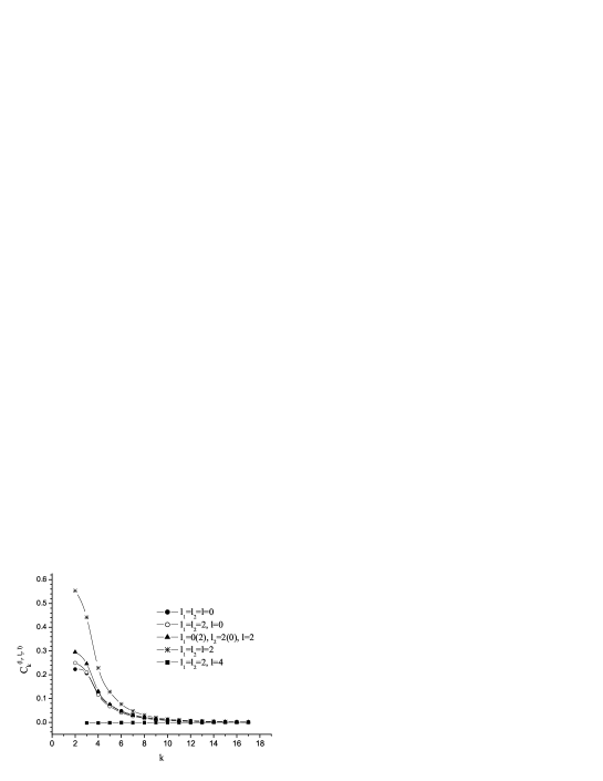
Figure 2: Ground state of ¹²Be: coefficients of the w.f. expansion in the $l$-basis

We were able to extract some information on the structure of the ground state of ¹²Be from the coefficients of the expansion of its wave function over the Pauli-allowed basis states (Fig. 2). Firstly, this nucleus appears to be softer than it would follow the results of the shell-model calculations. The standard shell-model configuration corresponds to the allowed state with the minimal number of quanta. The weight of this component in the g.s. wave function is only 54%. The considerable contribution of other states even at relatively large $k$ indicates the diffuseness of the nuclear surface and shows the correct asymptotic behavior of the wave function in each of the five closed channels.

Imitating the dependence of the wave function in the coordinate representation on the inter-cluster distance, the expansion coefficients fall exponentially with the number of quanta increasing. Asymptotically, in the $i$th $l$-channel,

$$C^{i}_{0}(k)\sim A^{i}_{0}\sqrt{2}\,{\exp\{-\sqrt{2(E_{i}-E_{0})}\sqrt{4k+3}\}\over{\sqrt[4]{4k+3}}},$$ (57)

where $E_{i}$ is the threshold energy for this channel, $E_{0}$ is the g.s. energy of ¹²Be. The factor $A^{i}_{0}$ is usually called ”asymptotic normalization coefficient” (ANC) [27].

The function of the channel ($l_{1}=l_{2}=l=2$) is characterized by the largest value of ANC, 43.49 fm^-1/2. In the channels ($l_{1}=l_{2}=l=0$), ($l_{1}=l_{2}=2,~{}l=0$) and ($l_{1}=2(0),l_{2}=0(2),~{}l=2$) the values of ANC are, respectively, 12.99 fm^-1/2, 25.61 fm^-1/2 and 19.1 fm^-1/2. The smallest ANC (0.8 fm^-1/2) is in the channel ($l_{1}=l_{2}=2,~{}l=4$).

Due to the large value of its ANC, the channel ($l_{1}=l_{2}=l=2$) is dominating in the g.s. function, with the weight 58%, despite the fact that its threshold is higher than those of ($l_{1}=l_{2}=l=0$) and ($l_{1}=2(0),l_{2}=0(2),~{}l=2$). The contributions of the latter channels are 12% and 17%, respectively. Those of the ($l_{1}=l_{2}=2,~{}l=0$) and ($l_{1}=l_{2}=2,~{}l=4$) channels are 13% and less than $10^{-5}\%$, respectively.

We also studied the expansion of the shell-model g.s. wave function of ¹²Be (the $(\lambda,\mu)=(2,0)$ function of the $SU(3)$ basis) in the $l$-basis. It is dominated by the ($l_{1}=l_{2}=l=2$) component – 60%, followed by ($l_{1}=2(0),~{}l_{2}=0(2),~{}l=2$) – $17.5\%$, ($l_{1}=l_{2}=2,~{}l=0$) – $12.5\%$, ($l_{1}=l_{2}=l=0$) – 10%.

8 Continuum part of the spectrum

In the approximation used here, the continuum part of the ¹²Be spectrum begins over the threshold of the decay into two ⁶He nuclei in their ground states. We set the energy of this threshold to zero. In the interval of energies $0<E<\epsilon$, the elastic scattering of two ⁶He nuclei is the only open channel, and all the information about this process is in the only $S$-matrix element $S_{11}=\exp(2i\delta_{11})$, i.e. in the scattering phase $\delta_{11}(E)$ (Fig. 3). The approximation and the limited, although infinite, basis provides for the existence of the sole bound state, therefore the phase $\delta_{11}(0)$ is set to $\pi$. In the vicinity of the threshold, the derivative of the phase with respect to the energy is inversely proportional to the square root of the energy, and the scattering length

$$a=-\lim{\delta_{11}(\kappa)\over\kappa}=6.62\mbox{fm},~{}~{}\kappa=\sqrt{2E}\rightarrow 0.$$

The phase steadily decreases with the energy increasing. Only a considerable rise in the intensity of the attractive potential can slow down this fall or force an increase.

Figure 3: Subthreshold elastic scattering in the channel ($l_{1}=l_{2}=l=0$).

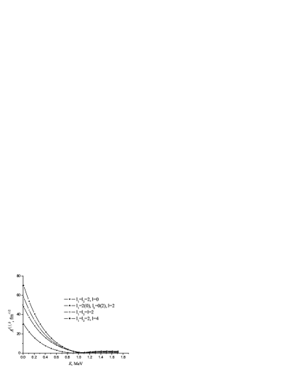
Figure 4: Asymptotic normalization coefficients (ANCs) in various exit channels. The entrance channel is ($l_{1}=l_{2}=l=0$).

As long as the energy is less than $\epsilon$, the behavior of the wave function in the closed channels is reproduced by the energy dependence of the four ANCs shown at Fig. 4. Their values are several times larger than those of the g.s. function. They reach their maxima just over the threshold (the largest ANC there, about 70 fm^-1/2, belongs to the ($l_{1}=l_{2}=2,l=4$) channel), and then they steadily fall, until the next threshold is reached.

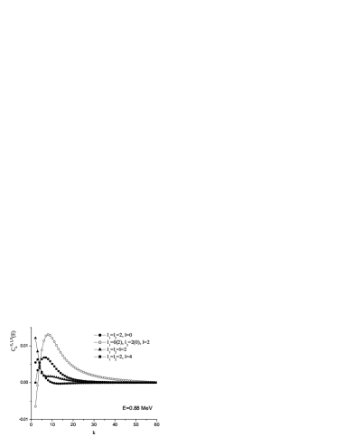
Figure 5: Coefficients $C^{(l_{1},l_{2},l)}_{k}(E)$ of the expansion of two continuum states (at $E=0.88$ MeV, left, and at $E=1.55$ MeV, right) in the $l$-basis

When the energy reaches $\epsilon=1.8$ MeV, the channel ($l_{1}=2(0),l_{2}=0(2),~{}l=2$) opens. Just below this threshold the wave function of this channel is expected to fall slower than those in other channels. Indeed (Fig. 5), the state ($l_{1}=2(0),l_{2}=0(2),~{}l=2$) dominates and has the longest tail. This dependence becomes more pronounced as the energy approaches the threshold.

Between the second and third thresholds the $S$-matrix has a standard two-channel form,

$$S=\left|\begin{array}[]{cc}S_{11}&S_{12}\\ S_{21}&S_{22}\end{array}\right|$$ (63)

$$S_{11}=\eta\exp(2i\delta_{11}),~{}~{}~{}S_{12}=i\sqrt{1-\eta^{2}}\exp(i\delta_{11}+i\delta_{22}),$$

$$S_{21}=i\sqrt{1-\eta^{2}}\exp(i\delta_{11}+i\delta_{22}),~{}~{}~{}S_{22}=\eta\exp(2i\delta_{22}).$$

In this energy region, $\epsilon<E<2\epsilon$, the three ANCs are an order of magnitude smaller than before. They depend not only on the energy, but also on which of the two open channels is the entrance one. Both dependences are illustrated at Fig. 6.

Figure 6: Asymptotic normalization coefficients (ANCs) in various exit channels in the energy domain between two thresholds. The entrance channel are ($l_{1}=l_{2}=l=0$) (left) and ($l_{1}=2(0),l_{2}=0(2),~{}l=2$) (right)

In the left panel of Fig. 6, the entrance channel is ($l_{1}=l_{2}=l=0$). The ANCs decrease monotonically with increasing energy, reaching their maximum values when $E-\epsilon$ is close to zero. When $E-\epsilon$ is small, the absolute values of the ANC in the channels ($l_{1}=l_{2}=2,l=4$) and ($l_{1}=l_{2}=l=2$) are almost twice larger than that in the channel ($l_{1}=l_{2}=2,l=0$).

If the entrance channel is ($l_{1}=2(0),l_{2}=0(2),~{}l=2$), the energy dependence is more interesting (Fig. 6, right panel). The ANCs in the channels ($l_{1}=l_{2}=2,~{}l=0$) and ($l_{1}=l_{2}=l=2$) have broad peaks at $E-\epsilon=1$ MeV, reaching 0.5 fm^-1/2 and 0.3 fm^-1/2, respectively, and then fall. In the ($l_{1}=l_{2}=2,~{}l=4$) channel, the ANC has a more pronounced maximum at $E-\epsilon=0.3$ MeV and than falls to almost zero. Such a behavior may indicate the existence of a resonance in this channel.

Above the third threshold, where $E>2\epsilon$, all the five channels are open, and the $S$-matrix is $5\times 5$. Having computed its elements, we found the effective cross-sections of elastic and inelastic scattering for energies up to 30 MeV.

The cross-section $\sigma_{11}$ of the elastic scattering in the channel ($l_{1}=l_{2}=l=0$) is shown at Fig. 7. It decreases smoothly from 5.1 b at $E=0.1$ MeV to 14 mb at $E=5$ MeV. There are no visible peculiarities at the thresholds $E=\epsilon$ and $E=2\epsilon$. However it is known that the existence of threshold reactions may be exhibited in a characteristic dependence of the elastic cross-section on the energy around the threshold (the Wigner–Baz’ effect[28]).

Figure 7: Cross-section of the elastic scattering in the channel ($l_{1}=l_{2}=l=0$). The breaks in the line indicate the decay thresholds

Consider the two-channel scattering matrix, Eq.(63). If, at $E=\epsilon$, there opens a channel with the relative orbital momenta $l$, then at small positive values of $E-\epsilon=\kappa_{1}^{2}/2$ the dependence of the inelasticity coefficient $\eta$ on the wave number $\kappa_{1}$ is defined by

$$\eta\sim 1-b\kappa_{1}^{2l+1}-...,~{}~{}b>0.$$

In this case, the elastic scattering in the energy region over the threshold $E=\epsilon$ should take the form

$$\sigma_{11}={4\pi\over\kappa^{2}}\sin^{2}\delta_{11}(1-a\kappa_{1}^{2l+1}-...).$$

Under this threshold, the $S$-matrix is reduced to a single value, and the cross-section follows the law

$$\sigma_{11}={4\pi\over\kappa^{2}}\sin^{2}\delta_{11}.$$ (64)

Therefore, at the threshold one may expect to see a change in the monotonic behavior. Evidently, this effect will be significant only if $l=0$. However, in the case considered here, $l=2$. So in order to study the Wigner–Baz’ effect we have checked the third threshold, $E=2\epsilon$, because one of the channels which open there has $l=0$. Still, there are no peculiarities in the cross-section. The explanation is following.

It appears that, in the expansion of the inelasticity coefficients $\eta_{1l}$ in the domain of small positive values of $E-2\epsilon=\kappa_{2}^{2}/2$, the first non-vanishing terms that define the behavior of the cross-sections are proportional to $b_{l}\kappa_{2}^{2l+3}$ rather than $b_{l}\kappa_{2}^{2l+1}$. Therefore, the Wigner-Baz’ effect will be less pronounced, and the following behavior is expected above the threshold $E=2\epsilon$,

$$\sigma_{1l}={\pi\over k^{2}}~{}b_{l}\left\{2(E-2\epsilon)\right\}^{l+3/2},~{}l=0,~{}2,~{}4.$$ (65)

Figure 8: Cross-sections of the inelastic scattering into the channels ($l_{1}=2(0),l_{2}=0(2),~{}l=2$) (left), and ($l_{1}=l_{2}=2,l=0,~{}2,~{}4$) (right). The entrance channel is ($l_{1}=l_{2}=l=0$)

In Fig. 8, inelastic cross-sections with the exit channels ($l_{1}=2(0),l_{2}=0(2),~{}l=2$) $(\sigma_{13})$ and ($l_{1}=l_{2}=2,l=0,~{}2,~{}4$) are compared. The behavior of the cross-sections does not indicate the existence of a resonance over the threshold ¹²Be$\rightarrow^{6}$He+⁶He up to several dozen MeV. The cross-section $\sigma_{13}$ has a broad maximum at 4.4 MeV over the threshold $E=\epsilon$, reaching 102 mb, and falls to 39 mb at $E-\epsilon=14$ MeV. Over the threshold $E=2\epsilon$, the exit channel ($l_{1}=l_{2}=2,~{}l=4$) dominates. The corresponding cross-section reaches 65 mb at $E-2\epsilon\sim 11$ MeV, while the other cross-sections do not exceed 12 mb.

9 Conclusions

Taking a system of two ⁶He clusters in ¹²Be as an example, we have shown that in the Fock–Bargmann space the eigenvalues of the norm kernel can be found by integrating its products with its eigenfunctions analytically. The latter are functions of the $SU(3)$ basis and can be constructed a priori, if there is no $SU(3)$-degeneracy. If there is one, the eigenfunctions are found as solutions of an integral equation with a degenerate kernel. When solving this equation, one uses standard algebraic procedures. An important detail is that the eigenvalues of this integral equation have a finite limiting point, where the eigenfunctions are defined with an accuracy up to a unitary transform. On the other hand, at any finite number of oscillator quanta $2k$ these functions are unique. At small $k$, eigenfunctions of a degenerate $SU(3)$ representation are related to their asymptotic counterparts (i.e., eigenfunctions at $k\rightarrow\infty$) via a rotation matrix. The angle of the rotation varies with $k$, changing the structure of the degenerate states.

The eigenvalues of the norm kernel limit to unity with $k$ increasing, with exponentially small corrections. Nevertheless, these corrections are important for the unique determination of the asymptotic eigenfunctions.

With the number of quanta increasing, the number of Pauli-allowed states grows from one (at $n=2k=4$) to five ($n\geq 10$).

Taking into account the Pauli principle leads to an effective potential related to the antisymmetrization. In the representation of the angular momentum-coupled $l$-basis, this potential consists of two terms. One of the terms determines the elastic scattering cross-section; it is a repulsion, the intensity of which is proportional to the energy of the continuum states and increases with the number of quanta decreasing. The scattering occurs over the barrier at any positive energy in all channels. The range of the repulsion is several times larger than the value of the oscillator radius, as deduced from the large scattering length and the elastic cross-section reaching several barn.

The second term influences the inelastic cross-sections. In the $l$-basis representation, the channels are coupled by the antisymmetrizer; the coupling falls exponentially with $k$ increasing, and the inelastic cross-sections are an order of magnitude smaller than the elastic one (several dozen mbarn).

In the representation of the $SU(3)$ basis, meanwhile, the channels are coupled not by the antisymmetrizer, but by the kinetic energy operator. With $k$ increasing, this coupling decreases more slowly, as $1/k$. The unitary transformation from the $SU(3)$ basis to the $l$-basis decouples the asymptotic equations of AVRGM, thus allowing to solve these equations in either basis.

Due to the Pauli principle, the wave functions of both the ground state and the continuum states of ¹²Be are distributed over several $l$-channels. The contribution of each channel is determined by the value of the normalization coefficient (related to the amplitude of the wave function in a closed channel) and by the proximity of the channel threshold. Thus the ground state wave function is dominated by the ($l_{1}=l_{2}=l=2$) channel due to its large normalization coefficient. It is also important to note the softness of the ¹²Be nucleus in comparison with the shell-model predictions.

The behavior of the normalization coefficients in the energy domain $\epsilon<E<2\epsilon$ of the continuum depends not only on the energy, but also on which of the two open channels is the entrance channel. A pronounced peak is observed in the dependence of the normalization coefficient on the energy in the channel ($l_{1}=l_{2}=2,~{}l=4$), provided that the entry channel is ⁶He$+^{6}$He^∗. This may signal the existence of a resonance in this channel.

The behavior of scattering phases does not indicate that there are resonances in any of the channels.

Appendix A $SU(3)$ invariants $F_{(\lambda,\mu)\nu}$

The norm kernel of ⁶He+⁶He can be expanded over $SU(3)$-scalar blocks $F_{(\lambda,\mu)\nu}$ (cf. Eq.(7)). Explicit expressions (Eq.4) for these invariants are shown below. A shorthand notation

$$\Phi_{(\lambda^{\prime},\mu^{\prime})\nu^{\prime}+\nu^{\prime\prime}}\equiv\Phi_{(\lambda^{\prime},\mu^{\prime})\nu^{\prime}}+\Phi_{(\lambda^{\prime},\mu^{\prime})\nu^{\prime\prime}}$$

is used.

$$F_{(n+4,0)} = {1\over 4n!}\left\{\Phi_{(n+4,0)}-{4\over n+4}\,\Phi_{(n+2,1)1}-{2\over n+4}\,\Phi_{(n+2,1)2+3}\right.+{2\over(n+3)(n+4)}\,\Phi_{(n,2)1}$$

$$+{n(n-1)\over(n+3)(n+4)}\,\Phi_{(n,2)2+3}+{4n(n-1)\over(n+3)(n+4)}\,\Phi_{(n,2)4}+{4n\over(n+3)(n+4)}\,\Phi_{(n,2)5+6}$$

$$-{2n(n-1)(n-2)\over(n+2)(n+3)(n+4)}\,\Phi_{(n-2,3)1+2}-{4n(n-1)\over(n+2)(n+3)(n+4)}\,\Phi_{(n-2,3)3}$$

$$+{n(n-1)(n-2)(n-3)\over(n+1)(n+2)(n+3)(n+4)}\,\Phi_{(n-4,4)}+{4n\over(n+3)(n+4)}\,\Phi_{(n+1,0)}$$

$$-{4n\over(n+2)(n+3)(n+4)}\,\Phi_{(n-1,1)1}-{4n(n-1)\over(n+2)(n+3)(n+4)}\,\Phi_{(n-1,1)2+3}$$

$$+{4n(n-1)(n-2)\over(n+1)(n+2)(n+3)(n+4)}\,\Phi_{(n-3,2)}$$

$$\left.+{2n(n-1)\over(n+1)(n+2)(n+3)(n+4)}\,\Phi_{(n-2,0)}\right\}$$

$$F_{(n+2,1)1} = {1\over 4n!}\left\{\Phi_{(n+2,1)1}-{1\over n+2}\,\Phi_{(n,2)1}-{n\over n+2}\,\Phi_{(n,2)5+6}+{n(n-1)\over(n+1)(n+2)}\,\Phi_{(n-2,3)3}\right.$$

$$-{n^{2}\over(n+2)(n+4)}\,\Phi_{(n+1,0)}+{2n\over(n+1)(n+4)}\,\Phi_{(n-1,1)1}$$

$$+{n^{2}(n-1)\over(n+1)(n+2)(n+4)}\,\Phi_{(n-1,1)2+3}-{n(n-1)(n-2)\over(n+1)(n+2)(n+4)}\,\Phi_{(n-3,2)}$$

$$\left.-{n(n-1)\over(n+1)(n+2)(n+4)}\,\Phi_{(n-2,0)}\right\}$$

$$F_{(n+2,1)2} = {1\over 4(n+4)(n-1)!}\left\{2\,\Phi_{(n+2,1)2+3}-\Phi_{(n+2,1)1}+{1\over n+2}\,\Phi_{(n,2)1}\right.$$

$$-{2(n-1)\over n+2}\,\Phi_{(n,2)2+3}-{8(n-1)\over n+2}\,\Phi_{(n,2)4}+{n-4\over n+2}\,\Phi_{(n,2)5+6}$$

$$+{6(n-1)(n-2)\over(n+1)(n+2)}\,\Phi_{(n-2,3)1+2}-{(n-1)(n-8)\over(n+1)(n+2)}\,\Phi_{(n-2,3)3}$$

$$-{4(n-1)(n-2)(n-3)\over n(n+1)(n+2)}\,\Phi_{(n-4,4)}+{n-4\over n+2}\,\Phi_{(n+1,0)}$$

$$-{2(n-2)\over(n+1)(n+2)}\,\Phi_{(n-1,1)1}-{(n-1)(n-8)\over(n+1)(n+2)}\,\Phi_{(n-1,1)2+3}$$

$$\left.+{(n-1)(n-2)(n-12)\over n(n+1)(n+2)}\,\Phi_{(n-3,2)}+{(n-1)(n-4)\over n(n+1)(n+2)}\,\Phi_{(n-2,0)}\right\}$$

$$F_{(n,2)1} = {1\over 12n!}\left\{\Phi_{(n,2)1}-{2n\over n+3}\,\Phi_{(n-1,1)1}+{n(n-1)\over(n+2)(n+3)}\,\Phi_{(n-2,0)}\right\}$$

$$F_{(n,2)2} = {1\over 8(n+2)(n-1)!}\left\{2\Phi_{(n,2)5+6}-\Phi_{(n,2)1}-{4(n-1)\over n}\,\Phi_{(n-2,3)3}-2\,\Phi_{(n+1,0)}\right.$$

$$+{2(n-1)(n+2)\over n(n+3)}\,\Phi_{(n-1,1)1}+{4(n-1)\over n(n+3)}\,\Phi_{(n-1,1)2+3}$$

$$\left.+{2(n-1)(n-2)\over n(n+3)}\,\Phi_{(n-3,2)}+{n-1\over n+3}\,\Phi_{(n-2,0)}\right\}$$

$$F_{(n,2)3} = {1\over 4(n+2)(n+3)(n-2)!}\left\{{1\over 6}\,\Phi_{(n,2)1}+\Phi_{(n,2)2+3}+4\,\Phi_{(n,2)4}-\Phi_{(n,2)5+6}\right.$$

$$-{6(n-2)\over n}\,\Phi_{(n-2,3)1+2}+{2(n-3)\over n}\,\Phi_{(n-2,3)3}+{6(n-2)(n-3)\over n(n-1)}\,\Phi_{(n-4,4)}$$

$$-\Phi_{(n+1,0)}-{n-6\over 3n}\,\Phi_{(n-1,1)1}+{2(n-3)\over n}\,\Phi_{(n-1,1)2+3}$$

$$\left.-{3(n-2)(n-5)\over n(n-1)}\,\Phi_{(n-3,2)}+{n^{2}-13n+24\over 6n(n-1)}\,\Phi_{(n-2,0)}\right\}$$

$$F_{(n-2,3)1} = {n-1\over 12(n+1)!}\left\{3\Phi_{(n-2,3)3}-\Phi_{(n-1,1)1+2+3}-{n-2\over n+2}\,\Phi_{(n-3,2)}-{n\over n+2}\,\Phi_{(n-2,0)}\right\}$$

$$F_{(n-2,3)2} = {(n-1)(n-2)\over 2(n+2)!}\left\{\Phi_{(n-2,3)1+2}-{1\over 2}\,\Phi_{(n-2,3)3}-{2(n-3)\over n-2}\,\Phi_{(n-4,4)}\right.$$

$$+{1\over 6}\,\Phi_{(n-1,1)1}-{1\over 2}\,\Phi_{(n-1,1)2+3}\left.-{n-2\over 3(n+2)}\,\Phi_{(n-3,2)}+{n\over 3(n+2)}\,\Phi_{(n-2,0)}\right\}$$

$$F_{(n-4,4)} = {n-3\over 4(n+1)!}\left\{\Phi_{(n-4,4)}-\Phi_{(n-3,2)}+{1\over 6}\,\Phi_{(n-2,0)}\right\}$$

$$F_{(n+1,0)} = {1\over 2(n+4)(n-1)!}\left\{\Phi_{(n+1,0)}-{1\over n+1}\,\Phi_{(n-1,1)1}-{n-1\over n+1}\,\Phi_{(n-1,1)2+3}\right.$$

$$\left.+{(n-1)(n-2)\over n(n+1)}\,\Phi_{(n-3,2)}+{n-1\over n(n+1)}\,\Phi_{(n-2,0)}\right\}$$

$$F_{(n-1,1)1} = {1\over 6(n+3)(n-1)!}\left\{\Phi_{(n-1,1)1}-{n-1\over(n+1)}\,\Phi_{(n-2,0)}\right\}$$

$$F_{(n-1,1)2} = {1\over 6(n+1)(n+3)(n-2)!}\left\{2\,\Phi_{(n-1,1)2+3}-\Phi_{(n-1,1)1}\right.$$

$$\left.-{4(n-2)\over n-1}\Phi_{(n-3,2)}+{n-3\over n-1}\,\Phi_{(n-2,0)}\right\}$$

$$F_{(n-3,2)} = {(n+1)(n-2)\over 4(n+2)!}\left\{\Phi_{(n-3,2)}-{1\over 2}\,\Phi_{(n-2,0)}\right\}$$

$$F_{(n-2,0)} = {n(n-1)\over 12(n+2)!}\,\Phi_{(n-2,0)}$$

Appendix B Coefficients $\lambda_{ij}(k)$

Coefficients $\lambda_{ij}(k)$ (see Eq.(18))

$$\lambda_{11}(k)=1-{4k^{3}+8k^{2}+19k+16\over 2(2k^{2}+k+1)}\left({4\over 9}\right)^{k}+{48k^{4}-32k^{3}-126k^{2}+47k+119\over 2k^{2}+k+1}\left({1\over 9}\right)^{k}$$

$$\lambda_{22}(k)=1-{4k^{4}+77k^{2}+9k+12\over 4(2k^{2}+k+1)}\left({4\over 9}\right)^{k}+{88k^{4}-200k^{3}+288k^{2}-75k+3\over 2k^{2}+k+1}\left({1\over 9}\right)^{k}$$

$$\lambda_{12}(k)={\sqrt{2k(2k-1)(k+1)(2k+3)}\over 4(2k^{2}+k+1)}\left\{(7-6k)\left({4\over 9}\right)^{k}-8(6k^{2}-25k+20)\left({1\over 9}\right)^{k}\right\}$$

References

• [1] Fujiwara, Y., Horiuchi, H.: Prog. Theor. Phys. 63, 895 (1980); 65, 1632, 1901 (1981)
• [2] Saito, S.: Suppl. Prog. Theor. Phys. 62, 895 (1977)
• [3] Horiuchi, H.: Eur. Phys. J. A13, 39 (2002)
• [4] Freer, M., et al.: Phys. Rev. Lett. 82, 1383 (1999)
• [5] Freer, M., et al.: Phys. Rev. C63, 034301 (2001)
• [6] Saito, A., et al.: Progr. Theor. Phys. Suppl. 146, 615 (2002)
• [7] Kanada-En’yo, Y., Progr. Theor. Phys. Suppl. 146, 190 (2002)
• [8] Kanada-En’yo, Y., Horiuchi, H.: Phys. Rev. C68, 014319 (2003)
• [9] Ito, M., Sakuragi, Y.: Phys. Rev. C62, 064310 (2000)
• [10] Descouvemont, P., Baye, D.: Phys. Lett. B505, 71 (2001)
• [11] Brink, D. M.: In: Proceeding of International School in Physics ”Enrico Fermi”, Course 36, p.247 (1966)
• [12] Bargmann, V.: Ann. Math. 48, 568 (1947)
• [13] Hecht, K. T., et al.: Nucl. Phys. A356, 146 (1981)
• [14] Kramer, P., Moshinsky, M., Seligman, T. H.: In: Group Theory and Its Applications, Vol. 3, (Loebl, E. M., ed.). New York: Academic Press 1975
• [15] Suzuki, Y., Reske, E. J., Hecht, K. T.: Nucl. Phys. A381, 77 (1982)
• [16] Draayer, J. P., Akiyama, Y.: J. Math. Phys. 14, 1904 (1973); Comput. Phys. Comm. 5, 405 (1973)
• [17] Hecht, K. T., Suzuki, Y.: J. Math. Phys. 24, 785 (1983)
• [18] Filippov, G. F., et al.: Few-Body Syst. (in print)
• [19] Harvey, M.: In: Advances in Nuclear Physics, Vol. 1, p.67. New York: Plenum Press 1973
• [20] Filippov, G. F., et. al: J. Math. Phys. 36, 4571 (1995)
• [21] Gradshteyn, I. S., Ryzhik, I. M.: Table of Integrals, Series, and Products. New York: Academic 1980
• [22] Filippov, G. F.: Riv. Nuovo Cim. 9, 1 (1989)
• [23] Filippov, G. F.: Sov. J. Nucl. Phys. 33, 928 (1981).
• [24] Varshalovich, D. A., Moskalev, A. N., Khersonkii, V. K.: Quantum Theory of Angular Momentum. World Scientific 1988.
• [25] Bethe, H. A., Morrison, P., Elementary Nuclear Theory. New York: Wiley 1956
• [26] Tanihata, I., et al., Phys. Lett. B206, 592 (1988)
• [27] Borbely, I., Blokhintsev, L. D., Dolinskii, E. I., Fiz. Elem. Chastits At. Yadra 8, 1189 (1977)
• [28] Baz’, A., Sov. Phys. – JETP 6, 709 (1958); 9, 1256 (1959)