A Test of X(5) for the $\gamma$ Degree of Freedom

Abstract

We present the first extensive test of the critical point symmetry X(5) for the $\gamma$ degree of freedom, based in part on recent measurements for the $\gamma$-band in ¹⁵²Sm. The agreement is good for some observables including the energies and most intra- and inter-band transitions, but there is also a serious discrepancy for one transition.

The recent 1 proposal of the critical point symmetry X(5) describing a vibrator to axial rotor first order phase transition has introduced a new paradigm into the arsenal of nuclear models and has generated considerable interest, both experimental and theoretical. Of course, no nucleus need exhibit exact agreement with such a symmetry. Since nuclei contain integer numbers of nucleons, their properties change discretely with $N$ and $Z$, and a transition region may well by-pass the exact critical point. Nevertheless, empirical examples of nuclei close to X(5) in structure were identified in ¹⁵²Sm 2 and ¹⁵⁰Nd 3 . Although X(5) is parameter-free (except for scale), the overall agreement with the data is quite good. A notable discrepancy in the absolute scale of inter-band $B(E2)$ values, discussed in detail in refs. 2 ; 4 , and very recently, in 5 , probably reflects the fact that these $N$ = 90 nuclei are slightly to the rotor side of the phase transition. Recently, other candidates for X(5) have been discussed 6 ; 7 ; 8 ; 9 .

To date, the X(5) predictions have been discussed primarily for the yrast and yrare degrees of freedom, that is, for the quasi-ground band and for the sequence of levels built on the $0^{+}_{2}$ level. However, the solution for the infinite square well (in $\beta$) ansatz underlying X(5) involves a separation of variables in the $\beta$ and $\gamma$ degrees of freedom, and leads to a full set of predictions for the quasi-$\gamma$-vibrational levels as well.

To date, the most significant comparison of X(5) predictions with data for the $\gamma$ degree of freedom was presented for ¹⁰⁴Mo 10 . It includes relative $\gamma$-band energies and several branching ratios. It is the purpose of the present Rapid Communication to exploit recent experiments using the GRID technique at the ILL and polarization measurements of $M1/E2$ mixing ratios at Yale 11 to present an extensive comparison of X(5) with $\gamma$-band data in ¹⁵²Sm, the first nucleus proposed to exhibit X(5) character. This comparison, including spins up to $9^{+}_{\gamma}$, about 15 absolute $B(E2)$ values, and a number of independent branching ratios, is the most thorough to date.

To compare these and other data on the $\gamma$-band in ¹⁵²Sm with X(5) one needs to explicitly solve the X(5) equation in $\gamma$. The starting point is the Bohr Hamiltonian

$$H=-\frac{\hbar^{2}}{2B}\left[\frac{1}{\beta^{4}}\frac{\partial}{\partial\beta}\beta^{4}\frac{\partial}{\partial\beta}+\frac{1}{\beta^{2}\sin 3\gamma}\frac{\partial}{\partial\gamma}\sin 3\gamma\frac{\partial}{\partial\gamma}-\frac{1}{4\beta^{2}}\sum_{\kappa}\frac{Q_{\kappa}^{2}(\Omega)}{\sin^{2}(\gamma-\frac{2\pi}{3}\kappa)}\right]+V(\beta,\gamma)~{},$$ (1)

with $V(\beta,\gamma)=V(\beta)+V(\gamma)$ 1 . The potential in $\beta$ is taken to be an infinite square well with $V(\beta)=0$ for $\beta\leq\beta_{W}$ and $V(\beta)=\infty$ for $\beta>\beta_{W}$, whereas the potential in $\gamma$ is assumed to be harmonic around $\gamma_{0}$ with $V(\gamma)=\frac{1}{2}C(\gamma-\gamma_{0})^{2}$. Approximate solutions can be obtained in the limit of small oscillations in the $\gamma$ variable combined with an adiabatic limit to separate the $\beta$ and $\gamma$ variables. The energy eigenvalues are given by

$$E(s,n_{\gamma},L,K)=E_{0}+a\,(x_{s,\nu})^{2}+b\,(n_{\gamma}+1)~{},$$ (2)

where $x_{s,\nu}$ is the $s$-th zero of a cylindrical Bessel function $J_{\nu}(x)$ with

$$\nu=\sqrt{\frac{L(L+1)-K^{2}}{3}+\frac{9}{4}}~{}.$$ (3)

For $K=0$ this form reduces to the result obtained in 1 . We note that this solution is valid for both the prolate ($\gamma_{0}=0$) and the oblate case ($\gamma_{0}=\pi/3$) due to the appearance of the irrotational moments of inertia in the Bohr Hamiltonian which vanish about the symmetry axes. There is an important difference with the moments of inertia of a rigid rotor, for which the relative sign of the $L(L+1)$ and $K^{2}$ terms would depend on whether the deformation is prolate or oblate 12 .

$B(E2)$ values can be obtained from the matrix elements of the quadrupole operator

$$T^{E2}=t\beta\left[{\cal D}^{(2)}_{\mu,0}(\Omega)\cos\gamma+\frac{1}{\sqrt{2}}\left({\cal D}^{(2)}_{\mu,2}(\Omega)+{\cal D}^{(2)}_{\mu,-2}(\Omega)\right)\sin\gamma\right]~{}.$$ (4)

The first term describes $\Delta K=0$ transitions and the second one $\Delta K=2$ transitions. The calculation of matrix elements of the quadrupole operator involves an integral over the Euler angles $\Omega$, and over the deformation variables $\beta$ and $\gamma$

$$B(E2;sn_{\gamma}LK\rightarrow s^{\prime}n_{\gamma}^{\prime}L^{\prime}K^{\prime})=\frac{5}{16\pi}\left<L,K,2,K^{\prime}-K|L^{\prime},K^{\prime}\right>^{2}\,B^{2}_{s\nu;s^{\prime}\nu^{\prime}}\,C^{2}_{n_{\gamma}K;n_{\gamma}^{\prime}K^{\prime}}~{},$$ (5)

where $B_{s\nu;s^{\prime}\nu^{\prime}}$ contains the integral over $\beta$ 1 , and $C_{n_{\gamma}K;n_{\gamma}^{\prime}K^{\prime}}$ over $\gamma$. In the derivation of the $B(E2)$ values of Eq. (5) we have, just as for the energies, assumed small oscillations in $\gamma$. For $\Delta K=0$ transitions the $\gamma$-integral reduces to the orthonormality condition of the wave functions in $\gamma$, i.e. $C_{n_{\gamma}K;n_{\gamma}^{\prime}K}=\delta_{n_{\gamma},n_{\gamma}^{\prime}}$, whereas for $\Delta K=2$ transitions this integral can be interpreted as an intrinsic transition matrix element.

The four independent coefficients that enter in the calculations, $B$, $\beta_{W}$, $C$ and $t$ can be determined from two excitation energies, e.g. $E_{2_{1}}$ and $E_{2_{\gamma}}$, and two B(E2) values for $\Delta K=0$ and $\Delta K=2$ transitions, $e.g.$, $B(E2;2_{1}\rightarrow 0_{1})$ and $B(E2;2_{\gamma}\rightarrow 0_{1})$.

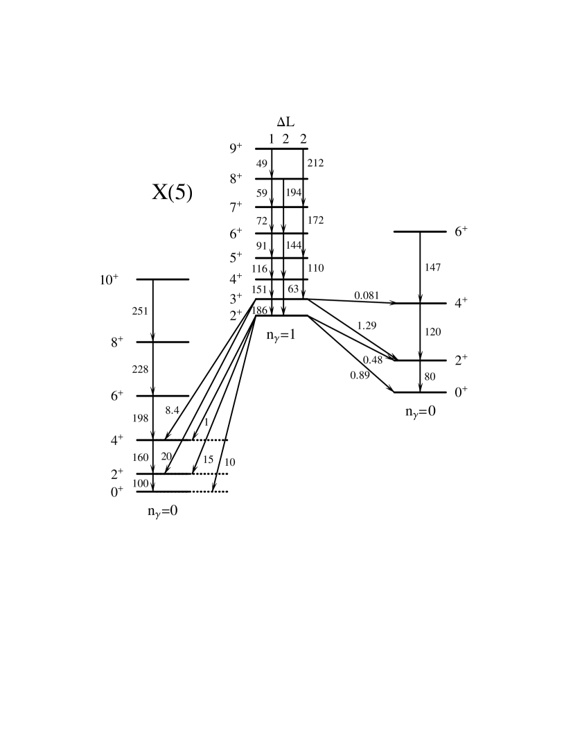
Figure 1: Predictions of X(5). The energy and $B(E2)$ values are normalized as in Tables I - IV. Here and in Fig. 2, the numbers on the transition arrows are $B(E2)$ values.

In Table I we present the X(5) results for the energies of the first two bands with $n_{\gamma}=0$, $K=0$, and the $\gamma$-band with $n_{\gamma}=1$, $K=2$. The moments of inertia of the ground band and the $\gamma$-band are almost identical, and much larger than that of the first excited $K=0$ band. The $B(E2)$ values for intraband transitions in the $\gamma$-band are shown in Table II, and those for interband transitions to the ground and 0${}^{+}_{2}$ bands in Tables III and IV. The values are normalized to the $\Delta K=0$ ground band transition $B(E2;2_{1}\rightarrow 0_{1})=100$ and the $\Delta K=2$ transition $B(E2;2_{\gamma}\rightarrow 0_{1})=10$, respectively. Many of these results are illustrated in Fig. 1. It is interesting to note that while the relative $\gamma-\gamma$ and $\gamma$-ground band $B(E2)$ values are close to the Alaga rules, the $\gamma\rightarrow$ 0${}^{+}_{2}$ band values differ significantly.

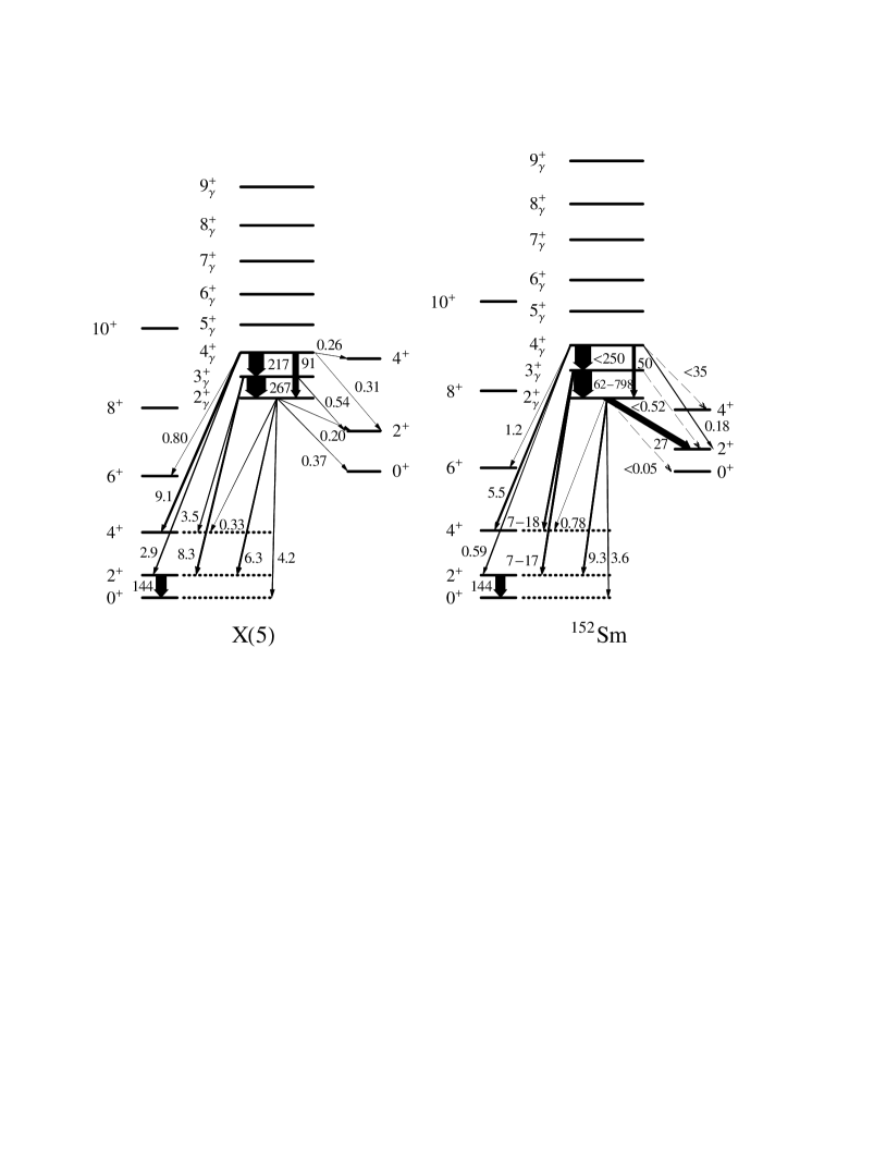
Figure 2: Comparison of the data for the quasi-$\gamma$-band in ¹⁵²Sm with X(5) predictions. Data from refs. 11 ; 13 ; 14 ; 15 ; 16 . See text. The thickness of the transition arrows indicates the corresponding $B(E2)$ values except that, for readability, the intraband transitions are scaled down in thickness by a factor of three. The numbers on the transition arrows are $B(E2)$ values in W.u. The dashed arrows on the right indicate transitions where only upper limits on the $B(E2)$ values are known.

Fig. 2 and Table V give a comparison with X(5) for all known quasi-$\gamma$-band energies and absolute $B(E2)$ values in ¹⁵²Sm. Table VI presents a comparison of the data with X(5) for cases where relative $B(E2)$ values are known. The data in these tables and Fig. 2 are taken from refs. 11 ; 13 ; 14 ; 15 ; 16 . The comparisons in Tables V, VI and Fig. 2, like other X(5) predictions, are parameter-free except for scale. As mentioned before, for the $\gamma$ degree of freedom, there are two additional scales that must be fixed beyond the normalization in Ref. 2 for the yrast and yrare levels. Thus, in Table V and Fig. 2 (left) we have normalized $E(2^{+}_{\gamma})$ to the experimental value and the $B(E2)$ values for the $\Delta K=2$ transitions to an average of the $2^{+}_{\gamma}\rightarrow 0^{+}_{1}$ and $2^{+}_{\gamma}\rightarrow 2^{+}_{1}$ transitions. The $\gamma\rightarrow\gamma$ in-band transitions have the same normalization as for the $\Delta K=0$ transitions among the yrast and yrare levels in ref. 2 , and are not affected by the scale factor for the $\Delta K=2$ transitions.

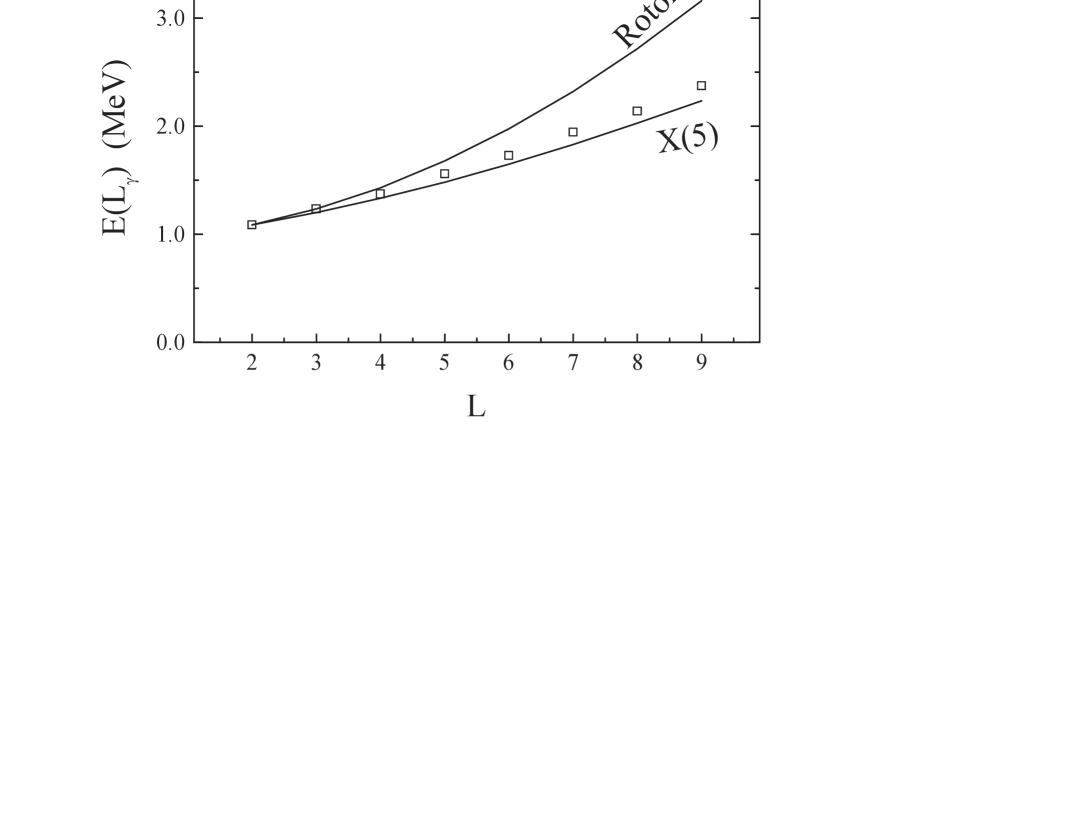
Figure 3: Comparison of relative $\gamma$-band energies in ¹⁵²Sm with X(5) and with an axial rotor.

The results are quite interesting. First, they provide an extensive test of X(5) for the $\gamma$-degree of freedom. Secondly, they exhibit both excellent agreement and at least one severe discrepancy. X(5) agrees quite well with the data for the $\gamma$-band energies, and far better than other paradigms such as the the axial rotor, as seen in Fig. 3. As with the yrast and yrare levels, ¹⁵²Sm deviates from X(5) slightly in the direction of the rotor. The spacings $within$ the odd-even spin couplets ($3^{+}_{\gamma}$, $4^{+}_{\gamma}$), ($5^{+}_{\gamma}$, $6^{+}_{\gamma}$), ($7^{+}_{\gamma}$, $8^{+}_{\gamma}$) are almost exact while the spacings $between$ couplets are slightly smaller in X(5) compared with the data.

Turning to transition rates, the three known intraband $B(E2)$ values in the quasi-$\gamma$-band are reasonably consistent with the data, and the $B(E2)$ values to the ground band are in rather good agreement. Of these latter transitions, the agreement is poorest for the $4^{+}_{\gamma}\rightarrow 2^{+}_{1}$, transition [0.59 (17) W.u. experimentally compared to 2.86 W.u. in X(5)]. Most of the transitions to the yrare, or $0^{+}_{2}$-band, levels are, experimentally, very weak (or else only upper limits are known), and so are the X(5) predictions. However, there is one glaring discrepancy, namely for the $2^{+}_{\gamma}\rightarrow 2^{+}_{2}$ transition, whose measured $B(E2)$ value 16 is 27(4) W.u., while X(5) predicts 0.20 W.u. The origin of this problem may be that, in the X(5) solution, the $\beta$ and $\gamma$ degrees of freedom are separated. In fact, calculations with both the IBA 16 and GCM 17 models, where their coupling is included, predict much higher $B(E2;2^{+}_{\gamma}\rightarrow 2^{+}_{1})$ values, which actually exceed the experimental ones. We noted earlier that the $\gamma\rightarrow$ 0${}^{+}_{2}$ band $B(E2)$ values differ significantly from the Alaga rules. The branching ratio from the 4${}^{+}_{\gamma}$ level ($<$ 0.7) is consistent with X(5) (0.84) but differs from the Alaga rule (2.93). It would clearly be of interest to measure relative $B(E2)$ values from higher lying members of the quasi-$\gamma$-band to further test the X(5) predictions.

Finally, the comparison of branching ratios in Table VI (where absolute rates are not known or poorly known) shows mixed agreement. The very small values, which are ratios of interband transitions to the ground band to intra-quasi-$\gamma$ band transitions, are likewise very small in X(5) and in good agreement with the data. However, for the three cases of branching ratios to the ground band, the experimental ratios are about 3–6 times larger than in X(5).

Overall, considering that X(5) is an invariant paradigm based on an infinite square well potential in $\beta$ and a harmonic potential in $\gamma$ that is parameter free (except for scale), the agreement is quite good. At the same time, the striking disagreement for the $2^{+}_{\gamma}\rightarrow 2^{+}_{2}$ transition needs to be better understood. Another area worth investigating are other forms of $V(\beta)$ 18 and/or $V(\gamma)$, in particular their effects on energies and $B(E2)$ values.

$L$	$E_{1}$($n_{\gamma}$ = 0)	$E_{2}$($n_{\gamma}$ = 0)	$E_{1}$($n_{\gamma}$ = 1)
0	0	565
2	100	745	1000
3			1094
4	290	1069	1204
5			1327
6	543	1475	1464
7			1613
8	848	1944	1774
9			1946
10	1203	2469	2131
11			2327
12	1604	3045	2534
13			2753
14	2051	3672	2983
15			3225
16	2544	4348	3477

Table 1: Excitation energies in X(5). The energies are normalized to E${}_{2_{1}}$ = 100 and E${}_{2_{\gamma}}$ = 1000.

$L_{\gamma}\rightarrow$	($L$ - 2)γ	($L$ - 1)γ
3γ		186
4γ	63	151
5γ	110	116
6γ	144	91
7γ	172	72
8γ	194	59
9γ	212	49
10γ	227	42

Table 2: B(E2) values for transitions within the quasi-$\gamma$-band for X(5). These values are normalized to the ground band transition B(E2; 2₁ $\rightarrow$ 0₁) = 100.

$L_{\gamma}\rightarrow$	($L$ - 2)1	($L$ - 1)1	$L_{1}$	($L$ + 1)1	($L$ + 2)1
2${}^{+}_{\gamma}$	10		15		0.78
3${}^{+}_{\gamma}$		20		8.4
4${}^{+}_{\gamma}$	6.8		22		1.9
5${}^{+}_{\gamma}$		20		12
6${}^{+}_{\gamma}$	6.3		25		2.7
7${}^{+}_{\gamma}$		21		14
8${}^{+}_{\gamma}$	6.2		27		3.3
9${}^{+}_{\gamma}$		22		16
10${}^{+}_{\gamma}$	6.3		29		3.7

Table 3: B(E2) values for transitions from the quasi-$\gamma$-band to the ground band for X(5). These values are normalized to the transition B(E2; 2_γ $\rightarrow$ 0₁) = 10.

$L_{\gamma}\rightarrow$	($L$ - 2)2	($L$ - 1)2	$L_{2}$	($L$ + 1)2	($L$ + 2)2
2${}^{+}_{\gamma}$	0.89		0.48		0.001
3${}^{+}_{\gamma}$		1.29		0.081
4${}^{+}_{\gamma}$	0.73		0.61		0.002
5${}^{+}_{\gamma}$		1.10		0.10
6${}^{+}_{\gamma}$	0.55		0.58		0.003
7${}^{+}_{\gamma}$		0.91		0.11
8${}^{+}_{\gamma}$	0.42		0.52		0.004
9${}^{+}_{\gamma}$		0.75		0.11
10${}^{+}_{\gamma}$	0.33		0.46		0.005

Table 4: B(E2) values for transitions from the quasi-$\gamma$-band to the 0${}^{+}_{2}$ band for X(5). These values are normalized to the transition B(E2; 2_γ $\rightarrow$ 0₁) = 10.

$J_{i}\rightarrow J_{f}$	$B(E2)$ W.u.
	Exp.	X(5)
2${}^{+}_{\gamma}\rightarrow$ 0${}^{+}_{1}$	3.62 (17)	4.20
$2^{+}_{1}$	9.3 (5)	6.33
4${}^{+}_{1}$	0.78 (5)	0.33
0${}^{+}_{2}$	$<$ 0.05	0.37
2${}^{+}_{2}$	27 (4)	0.20
3${}^{+}_{\gamma}\rightarrow$ 2${}^{+}_{1}$	7 - 17	8.31
4${}^{+}_{1}$	7 - 18	3.51
2${}^{+}_{2}$	$<$ 0.52	0.54
2${}^{+}_{\gamma}$	62 - 798	267.2
4${}^{+}_{\gamma}\rightarrow$ 2${}^{+}_{1}$	0.59 (17)	2.85
4${}^{+}_{1}$	5.5 (16)	9.05
6${}^{+}_{1}$	1.2 (4)	0.80
2${}^{+}_{2}$	0.18 (7)	0.31
4${}^{+}_{2}$	$<$ 35	0.26
2${}^{+}_{\gamma}$	50 (15)	90.7
3${}^{+}_{\gamma}$	$<$ 250	217.3

Table 5: Comparison of absolute $B(E2)$ values for the quasi-$\gamma$-band in ¹⁵²Sm with X(5). The scale for $\Delta K=2$ transitions is normalized to approximately reproduce the $2^{+}_{\gamma}\rightarrow 0^{+}_{1}$ and $2^{+}_{\gamma}\rightarrow 2^{+}_{1}$ B(E2) values. Data are from refs. 5 ; 7 ; 8 ; 9 ; 10 .

$B(E2)$ Ratio	Exp.	X(5)
3${}^{+}_{1}\rightarrow$ 4${}^{+}_{1}$ / 3${}^{+}_{1}\rightarrow$ 2${}^{+}_{1}$	1.08 (1)	0.42
5${}^{+}_{\gamma}\rightarrow$ 4${}^{+}_{1}$ / 5${}^{+}_{\gamma}\rightarrow$ 3${}^{+}_{\gamma}$	0.039 (13)	0.054
6${}^{+}_{\gamma}\rightarrow$ 6${}^{+}_{1}$ / 6${}^{+}_{\gamma}\rightarrow$ 4${}^{+}_{1}$	23 (8)	3.95
7${}^{+}_{\gamma}\rightarrow$ 8${}^{+}_{1}$ / 7${}^{+}_{\gamma}\rightarrow$ 6${}^{+}_{1}$	4.1 (14)	0.69
7${}^{+}_{\gamma}\rightarrow$ 6${}^{+}_{1}$ / 7${}^{+}_{\gamma}\rightarrow$ 5${}^{+}_{\gamma}$	0.0099 (17)	0.036
9${}^{+}_{\gamma}\rightarrow$ 10${}^{+}_{1}$ / 9${}^{+}_{\gamma}\rightarrow$ 7${}^{+}_{\gamma}$	0.021 (21)	0.022

Table 6: Comparison of B(E2) branching ratios (where $M1/E2$ mixing ratios are known) for the quasi-$\gamma$-band in ¹⁵²Sm with X(5) (for levels with unknown (or poorly known) lifetimes or absolute $B(E2)$ values). Data are from refs. 5 ; 7 ; 8 ; 9 .

References

- (1) F. Iachello, Phys. Rev. Lett. 87, 052502 (2001).
- (2) R.F. Casten and N.V. Zamfir, Phys. Rev. Lett. 87, 052503 (2001).
- (3) R. Krücken et al., Phys. Rev. Lett. 88, 232501 (2002).
- (4) R.M. Clark et al., Phys. Rev. C67, 041302(R) (2003).
- (5) R.F. Casten, N.V. Zamfir, and R. Krücken, Phys. Rev. C,in press.
- (6) M.A. Caprio et al., Phys. Rev. C66, 054310 (2002).
- (7) R.M. Clark et al., Phys. Rev. C68, 037301 (2003).
- (8) E.A. McCutchan et al., in Proc. of Int. Conf. on Symmetries in Nuclear Structure, Ettore Majorana Centre, Erice - March 23-29, 2003, in press; E.A. McCutchan et al., to be published.
- (9) C. Hutter et al., Phys. Rev. C67, 054315 (2003).
- (10) P.G. Bizzeti and A.M. Bizzeti-Sona, Phys. Rev. C66, 031301(R) (2002).
- (11) N.V. Zamfir et al., Phys. Rev. C65, 067305 (2002).
- (12) F. Iachello, private communication.
- (13) J. Konijn et al., Nucl. Phys. A 373, 397 (1982).
- (14) A. Artna–Cohen, Nucl. Data Sheets 79, 1 (1996).
- (15) N.M. Stewart, E. Eid, M.S.S. El–Daghmah, J.K. Jabben, Z. Phys. A 335, 13 (1990).
- (16) N.V. Zamfir et al., Phys. Rev. C60, 054312 (1999).
- (17) J.-Y. Zhang, M.A. Caprio, N.V. Zamfir, and R.F. Casten, Phys. Rev. C60, 061304(R) (1999).
- (18) N. Pietralla and O.M. Gorbachenko, preprint.