Correlation energies by the generator coordinate method:
computational aspects for quadrupolar deformations

Abstract

We investigate truncation schemes to reduce the computational cost of calculating correlations by the generator coordinate method based on mean-field wave functions. As our test nuclei, we take examples for which accurate calculations are available. These include a strongly deformed nucleus, ¹⁵⁶Sm, a nucleus with strong pairing, ¹²⁰Sn, the krypton isotope chain which contains examples of soft deformations, and the lead isotope chain which includes the doubly magic ²⁰⁸Pb. We find that the Gaussian overlap approximation for angular momentum projection is effective and reduces the computational cost by an order of magnitude. Cost savings in the deformation degrees of freedom are harder to realize. A straightforward Gaussian overlap approximation can be applied rather reliably to angular-momentum projected states based on configuration sets having the same sign deformation (prolate or oblate), but matrix elements between prolate and oblate deformations must be treated with more care. We propose a two-dimensional GOA using a triangulation procedure to treat the general case with both kinds of deformation. With the computational gains from these approximations, it should be feasible to carry out a systematic calculation of correlation energies for the nuclear mass table.

I Introduction

Much progress has been made in developing a fully microscopic method to determine nuclear binding energies. The most successful approach in this framework go02 starts from an energy functional of the nuclear orbitals BHR03 , which is minimized by solving mean-field equations for the orbitals. However, to achieve a level of accuracy around 700 keV on the more than 2000 known masses, some correlation energies beyond what can be subsumed within the mean-field functionals have to be introduced. Unfortunately, the well-established microscopic methods which could be applied are far too costly to be used for such a large number of nuclei. As a consequence, in the systematics of binding energies, the effects of correlations are estimated with phenomenological methods whose range of validity is not apparent. Our goal is find microscopically founded yet easy-to-implement methods allowing an accurate calculation of these correlations.

There are several systematic approaches to correlation energies. Among them, the generator coordinate method BHR03 is especially promising, mainly because of two attractive features: it is a fully variational method and it is not limited to small-amplitude collective motion. It has been used successfully by the Paris-Brussels collaboration for calculating spectroscopic properties of nuclei (for representative applications, see Refs. bo91 ; HBD93 ; MBW95 ; HVB01 ; va00 ; be03 ; du03 ; BFH03 ), and we believe it has promise for a global microscopic theory to systematically calculate nuclear masses.

The most important fluctuations beyond the mean field are those associated with pairing fluctuations and with quadrupolar deformations. We only discuss the latter in this work; the pairing fluctuations are treated by number projection as in the above cited GCM studies. At the mean-field level, quadrupolar deformations are introduced by using a quadrupolar constraining field to generate deformed configurations. To go beyond the mean field, one mixes configurations to obtain an additional correlation energy. This can happen in two ways. First, whenever the mean-field minimum is deformed, it can be interpreted as the intrinsic state of a rotational band. The lowest mean-field energy then corresponds to a weighted average over the members of the band, and one gains correlation energy by projecting onto the ground state of the band. Second, fluctuations of the quadrupole deformation about the value of the mean-field energy minimum also contribute to the correlation energy. In fact, when that minimum is spherical, they are the only one present. Both kind of correlations can be introduced simultaneously by projecting good angular momentum from the intrinsic states and by mixing configurations around the mean-field energy minimum with the generator coordinate method with the quadrupolar deformation as generator coordinate. Note that because the resulting wave function has amplitudes for deformed as well as spherical configurations, the distinction between these two correlations becomes blurred.

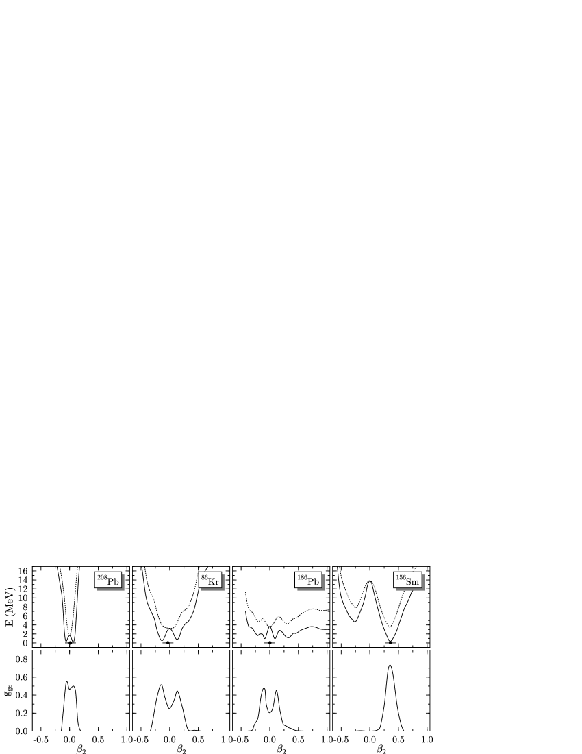
Figure 1: Overview of potential energy landscapes for selected nuclei. See text for details.

In previous works du03 ; be03 ; BFH03 ; va00 , the procedure to introduce these correlations consists of three steps. First one constructs mean-field wave functions for a set of configurations that are defined by a constraining quadrupolar field. These configurations may be labeled by the Bohr-Mottelson variables of two deformation parameters $\beta$ and $\gamma$. From them, additional states are generated by rotations with Euler angles $\Omega=(\phi,\theta,\chi)$ from which are projected states of good angular momentum. The projected states corresponding to different values of $\beta$ and $\gamma$ are then mixed by the GCM, which means numerically solving the Hill-Wheeler equations in the discrete basis of the projected configuration set. The computational issue in such calculations is in the selection of the Euler angles and the deformation parameters that are necessary to achieve a sufficient accuracy. Up to now, a fairly large number of active angles ($\sim 12$) were used for each deformation. We will show that this can be drastically simplified by using a suitable Gaussian overlap approximation, particularly the topological Gaussian overlap approximation advocated in ref. ha02 .

Figure 1 gives an overview of the energetics associated with the $\beta$ degree of freedom in selected nuclei. We have singled out ²⁰⁸Pb as an example of a doubly magic nucleus, ⁸⁶Kr as a soft spherical vibrator, ¹⁸⁶Pb as a soft nucleus with several coexisting near-degenerate minima, and ¹⁵⁶Sm as a well-deformed nucleus. The upper panel shows the energy surface, measuring the energy with respect to that of the GCM ground state. The dashed curve shows the energies of the states obtained by $N$ and $Z$ number projection from the HF+BCS configurations. The configurations are labeled by their intrinsic quadrupole moments

$$\beta_{2}=\frac{4\pi}{3Ar_{0}^{2}}\langle r^{2}\,Y_{20}\rangle$$ (1)

with $r_{0}=1.2\,A^{1/3}$ fm. In the figure, the states are connected by the line. One sees that the ground state is spherical except for ¹⁵⁶Sm, which has a strong prolate deformation. The solid curves show the results of angular momentum projection onto $J=0$, labeling the states by the deformation of the state from which they were projected. One sees that there is a net gain of energy using a deformed intrinsic configuration for all the nuclei including ²⁰⁸Pb. The final energy, obtained by the Hill-Wheeler equations using the $Z,N,J$-projected configurations, is at zero energy on the graph. The dot indicates the average deformation of the mean-field states within the Hill-Wheeler ground state. The lower panel shows the relative amplitudes of the different configurations in the ground-state wave function. For ¹⁵⁶Sm, the function has a single peak and can easily be interpreted as the zero-point motion of the $\beta$-vibration. For the other nuclei, there is a strong mixing of oblate and prolate configurations. As we will see below, this makes a simplified treatment for spherical nuclei somewhat more complicated than for the fully deformed nuclei.

The GOA has often been used in the past to derive the ingredients of a collective Bohr Hamiltonian in the spirit of the work of Kumar and Baranger Kum68 . It is supplemented by several other approximations BHR03 ; GG79 . The resulting Hamiltonian is five-dimensional, three dimensions corresponding to rotation and two to quadrupolar vibrations. This approach has been followed in ref. [14] and [15] to improve on the mean field theory of the Skyrme and Gogny interactions, respectively. The Lublin group has derived an alternative scheme starting from a Nilsson Hamiltonian go85 ; Pil93 ; pr99 , which allows one to introduce several collective degrees of freedom. In the present work, the GOA is a numerical approximation, in principle under control, used to evaluate matrix elements of the norm and Hamiltonian kernels of the generator coordinate method, including projection on good angular momentum.

Most previous calculations with the angular-momentum projected GCM have assumed axial symmetry, i.e. taking only configurations with $\gamma$ a multiple of $\pi/6$, and we will make the same assumption here. In practive, the optimal spacing of configurations as a function of $\beta$ remains to be determined, and also which off-diagonal matrix elements need to be calculated explicitly rather than estimated by the GOA. The first question was studied in ref. bo90 for unprojected matrix elements of the nucleus ¹⁹⁴Hg. We will see that the same considerations apply to the projected matrix elements, provided that the special characteristics of the $\beta=0$ singular point are taken into account.

In the next section, we examine several methods for the approximate angular projection. Our target is to design a procedure leading to an accuracy of a few hundred keV, the level required to improve the best present mean-field based approach to binding energies. We find that a two-point approximation gives acceptable accuracy in all but rare circumstances. In Section IV we discuss the mesh of GCM configurations entering the Hill-Wheeler equation, and we propose a prescription for simplifying the space without losing the desired accuracy.

Let us now briefly describe our procedure for dealing with pairing fluctuations. The mean-field calculations are performed in the Hartree-Fock+BCS approximation using the Skyrme interaction for the particle-hole channel field and a separate zero-range interaction for the pairing channel. The mean-field interaction is taken to be the SLy6 parameterization in the present work, the same as was used in ref. du03 . The pairing interaction is taken as a density-dependent delta function as in ref. ri99 ; it is used with 5 MeV cut-off of the orbital space above and below the Fermi energy. We use the same strength of the pairing as in ref. ri99 , (-1250 MeV fm³), except for the Kr isotopes, where it taken as -1000 MeV fm³. To avoid the phase transition of the BCS theory at nuclei with low densities of state at the Fermi surface, the Lipkin-Nogami prescription is used to generate the BCS wave functions, which are then projected onto fixed numbers of protons and neutrons. The last step is essential to have nuclide-specific predictions. We always use number-projected wave functions in this work, and will refer to them as the intrinsic configurations of the GCM to distinguish them from the BCS configurations that do not have definite particle numbers.

II Angular projection

The angular projection of a deformed wave function is carried out by calculating the integral

$$I_{0}(q,q^{\prime})=2\int_{0}^{1}d\cos(\theta)\langle q|R_{\theta}|q^{\prime}\rangle$$ (2)

and similar expressions for the matrix elements of the Hamiltonian and other operators. Here we have used the axial symmetry and the symmetry with respect to $180^{\circ}$ rotations, $\langle q|R_{\theta}|q^{\prime}\rangle=\langle q|R_{\pi-\theta}|q^{\prime}\rangle$, to reduce the integration over Euler angles to the above single integral. These properties can be used if the left and right wave functions have the same symmetry axes. We shall define our intrinsic configurations accordingly, taking the symmetry axis along $z$. This requires that the oblate wave functions correspond to $\gamma=180^{\circ}$ instead of the usual $60^{\circ}$.

In ref. du03 the integration was carried out on a Gauss-Legendre mesh with enough points to thoroughly sample the integrand in the range that it is nonzero. This is done in such a way that using the estimate for the overlap given in Ref. ba86 , the total number of abscissas in the interval $[-1,1]$ is chosen in such a way that at least 12 abscissas can be expected to give overlaps that are larger than $10^{-8}$ times the overlap at $\theta=0$. The calculation of the integrand is started at $\theta=0$ and stopped when the calculated overlap has indeed fallen below this value. In this way, the choice of the Gauss-Legendre mesh is self-adjusting to the structure of the integrand, which scales with the dispersion of the angular momentum and is therefore nearly constant for states with small deformation and sharply peaked at $\theta=0$ for well-deformed ones.

As discussed in the Appendix, the rotation operation is a rather costly computational task. The Gaussian overlap approximation reduces the number of points to one (besides the identity), making it attractive for global applications. There are a number of ways that the approximation can be applied. We shall write a generalized GOA for the overlap in the form

$$\langle q|R_{\theta}|q^{\prime}\rangle=\langle q|q^{\prime}\rangle\,e^{-c(q,q^{\prime})\,F(\theta)}$$ (3)

where $F$ has a fixed functional dependence on $\theta$. Since there is only parameter in the expression, namely $c(q,q^{\prime})$, only one rotation and many-particle overlap has to be carried out to determine it. The integral over the Gaussian is then a trivial computational task.

The naive GOA takes $F(\theta)=\theta^{2}$, which was proposed in early papers on the subject vi71 ; is79 . Another form suggested in ref. ba84 is $F=1-\cos(\theta)$. We will call this the improved GOA. It is designed for cranking wave functions which break the time-reversal invariance. In our case here, the wave functions are invariant under time reversal and have additional rotational symmetries as well. With quadrupolar amplitudes to be rotated, a form having the correct limit for small deformations is is79

$$\langle q|R_{\theta}|q^{\prime}\rangle=\exp\big{\{}-\sum c_{m,m^{\prime}}\big{[}\delta_{m,m^{\prime}}-{\cal D}^{2}_{m,m^{\prime}}(\Omega)\big{]}\big{\}}$$

where ${\cal D}^{2}$ is Wigner’s rotation matrix for $J=2$. Hagino et al. ha02 have considered this form for the case of axial symmetry, taking $F$ as

$$F=\sin^{2}(\theta)\sim 1-{\cal D}^{2}_{0,0}.$$ (4)

Testing the approximation in a three-level Lipkin model, they found an important gain in accuracy using the $\sin^{2}(\theta)$ dependence, which they call “topological GOA” (topGOA). They also tested the approximation on the Interacting Boson Model and found similar improvement ha03 .

We show in Fig. 2 the overlap $\langle q|R_{\theta}|q\rangle$ as a function of angle for a case of moderate deformation, ²⁰⁸Pb at a deformation of -5 b ($\beta_{2}=-0.063$). The points were calculated with the full many-particle wave functions. The GOA is constructed using the overlap at $\cos(\theta)=0.75$, where it is close to 0.5. The curves show the fits with the improved GOA and with the topGOA. While the improved GOA loses accuracy away from the peak, the topGOA gives a reasonable fit throughout. The projected integral $I_{0}$ is off by 18$\%$ for the improved GOA and only 1.3$\%$ for the topGOA.

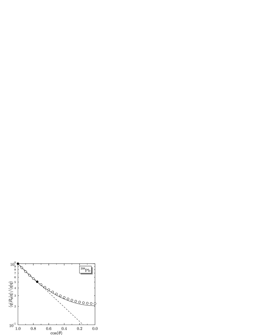
Figure 2: The overlap $\langle q|R_{\theta}|q\rangle$ for the nucleus ²⁰⁸Pb at $q=500$ fm². The overlaps of the particle-number projected BCS intrinsic states have been renormalized to one at $\theta=0$. The circles show the full calculation with the rotated many-particle wave functions. The fit by the topGOA is shown by the solid line and the fit by the improved GOA is shown as the dashed line. The $\theta=0$ point and the point shown as the filled circle were used to make the fit.

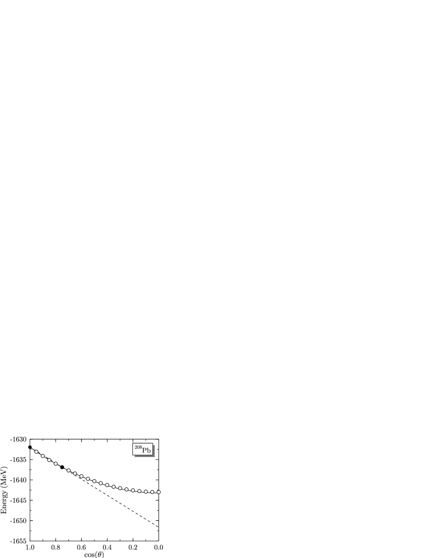
Figure 3: Hamiltonian matrix element as a function of rotation angle for ²⁰⁸Pb at $q=-500$ fm². The circles show the calculated values with the full many-particle wave function, and the lines are fits to the forms $h_{0}-h_{2}\sin^{2}(\theta)$ (solid) and $h_{0}-h_{2}(1.0-\cos\theta)$ (dashed). The two filled circles show the matrix elements that were used for the fit.

Next we consider the Hamiltonian matrix elements and their projection. Part of the GOA scheme as is usually applied assumes that the Hamiltonian matrix elements can be written as a product of the overlap times a factor that is quadratic in the difference of generator coordinates. For all versions of the GOA this may be expressed

$$\langle q|HR_{\theta}|q^{\prime}\rangle=\langle q|q^{\prime}\rangle\,e^{-c(q,q^{\prime})F(\theta)}\Big{[}h_{0}(q,q^{\prime})-h_{2}(q,q^{\prime})F(\theta)\Big{]}$$ (5)

The values of $h_{0}$ and $h_{2}$ may be determined from the two Hamiltonian matrix elements at $\theta=0$ and at the value used before to determine $c$. In Fig. 3 we show how well this works in the ²⁰⁸Pb example. Plotted as circles are the ratios $\langle q|HR_{\theta}|q\rangle/\langle q|R_{\theta}|q\rangle$ calculated from the many-particle wave functions. The fits by the improved GOA and the topGOA are shown as curves. Again the topGOA is superior at the moderate deformation of this example.

We now carry out the integrals to get the angular momentum projected energies

$$E_{qq^{\prime},J=0}=2\,I^{-1}_{0}(q,q^{\prime})\int_{0}^{1}d\cos(\theta)\,\langle q|HR_{\theta}|q^{\prime}\rangle.$$ (6)

We report here the diagonal correlation energies $\Delta E_{q,proj}$ defined by the difference in the projected energy and the energy of the intrinsic configuration,

$$\Delta E_{q,proj}=E_{qq,J=0}-\langle q|H|q\rangle.$$

Later, we shall present the energy difference with respect to the minimum energy of the unprojected configurations,

$$\Delta E_{corr}=\min_{q}E_{qq,J=0}-\min_{q}\langle q|H|q\rangle.$$ (7)

This correlation energy is more useful to assess the effect of the projection on the calculation of the ground state binding energy.

For the case presented in Figs. 2 and 3, the energy gained by projection is 5.8 MeV for the accurate integration, and essentially the same value for the GOA. In this case, both the topGOA and the naive GOA give values within 0.1 MeV of each other. In Fig. 4 we show the comparison of the (numerically converged) 12-point projection with the GOA for a number of other nuclei and deformations.

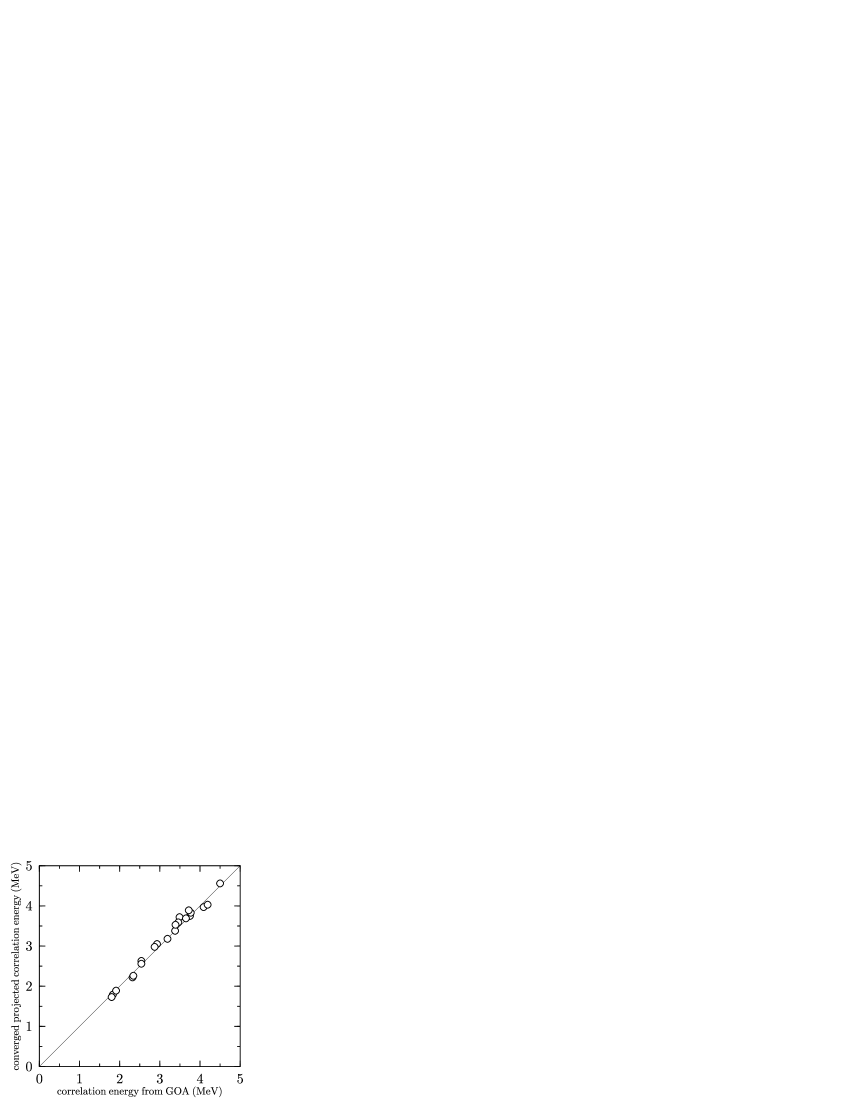
Figure 4: Comparison of explicit and GOA calculations of the projection, for the nuclei ¹²⁰Sn and ¹⁵⁶Sm and a number of deformations.

The correlation energy associated with the angular momentum projection has a range of about 2 to 4 MeV, with the larger values occurring for well-deformed configurations. The topGOA tracks these values closely, with a typical error of the order of 100-200 keV.

In the above, we only examined overlaps and matrix elements between configurations with the same sign of deformation. These quantities are of course also needed for matrix elements between oblate and prolate configurations. However, due to the choice of the same symmetry axis for oblate and prolate configurations, the overlap function has a rather different appearance. An example is shown in Fig. 5, the overlap between the configurations $q=500$ and $-500$ fm² of the nucleus ²⁰⁸Pb. Here we see that the overlap peaks at 90^∘. This is not surprising. The maximum density overlap is obtained by aligning the long axis of the prolate ellipsoid to one of the longer axes of the oblate ellipsoid. This requires rotating one of the ellipsoids by 90^∘. We may continue to use the functional form of the topGOA in this case, but the first point should be taken where the overlap is maximum. Thus, two rotations are needed, a first one by 90^∘ for the maximum, which is equivalent to a permutation of axes, and at some intermediate angle to get the width of the Gaussian. The curve in Fig. 5 shows the fit obtained using the two points shown by filled circles.

Figure 5: Same as Fig. 2, for the off-diagonal overlap $\langle q|R_{\theta}|q^{\prime}\rangle$ with $q=500$ fm² and $q^{\prime}=-500$ fm², which corresponds to $|\beta_{2}|=0.063$.

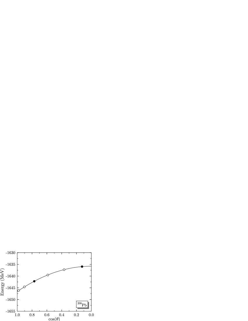
Figure 6: Same as Fig. 3, for the off-diagonal Hamiltonian matrix element $\langle q|HR_{\theta}|q^{\prime}\rangle$ with $q=500$ fm² and $q^{\prime}=-500$ fm².

We determine the two parameters of the Hamiltonian matrix elements, eq. (5), using the same two angles. The fit is compared to the numerically calculated values in Fig. 6. We can define a correlation energy for the off-diagonal matrix elements similar to the definition for diagonal elements,

$$\Delta E_{q,-q^{\prime};proj}=E_{q,-q^{\prime};J=0}-{\langle q|HR_{\pi/2}|-q^{\prime}\rangle\over\langle q|R_{\pi/2}|-q^{\prime}\rangle}.$$

For the case presented in Figs. 5 and 6, the value calculated with the fine angular mesh is 2.50 MeV, to be compared with 2.49 MeV estimated by the topGOA. For crossover matrix elements such as this one, one should not expand about $\theta=0$ using a nontopological GOA.

It is possible to use one of the other GOA’s if one makes a rotation of one of the intrinsic configurations by $90^{o}$ to align the longer axes. Calling the rotated wave function $|q,\pi/2\rangle\equiv R_{\pi/2}|q\rangle$, the overlap integral becomes

$$I_{0}(q,q^{\prime})=2\int_{0}^{1}d\sin(\theta)\langle q,\pi/2|R_{\theta}|q^{\prime}\rangle.$$ (8)

In this representation, the improved GOA gives a value for the overlap which differs by less than 1% from the value obtained by 12-point Gauss-Legendre integration. Note that topGOA gives identical values with either eq. (2) or (8).

III Mixing deformations

In the previous section, we have presented a numerical approximation which allows one to calculate the matrix element projected on $J=0$ between any two intrinsic configurations $(q,q^{\prime})$. If the total number of configurations is $N$, one needs $N(N+1)/2$ elements per matrix. In this section, we introduce an approximation scheme which requires only that diagonal and nearest-neighbor off-diagonal matrix elements be calculated with the full many-particle wave functions. This reduces the number of needed elements to $2N-1$, giving considerable savings in computational cost.

The diagonalization of the discretized Hill-Wheeler equations is equivalent to the variational theory based on a wave function of the form

$$|\Psi\rangle=\sum_{i}c_{i}\,|q_{i},0\rangle,$$

where the $c_{i}$ are variational parameters and $|q_{i},0\rangle$ are the $J$-projected intrinsic configurations. The total energy is thus

$$E_{HW}=\min_{c_{i}}{\langle\Psi|H|\Psi\rangle\over\langle\Psi|\Psi\rangle}$$

and the energy gained by configuration mixing is

$$\Delta E_{HW}=E_{HW}-\min_{q}E_{qq,J=0}.$$ (9)

As mentioned earlier, the configurational basis only includes axially symmetric deformations. For a given sign of the deformation (prolate or oblate), the intrinsic states can be ordered with respect to their quadrupole moments. The diagonal and nearest-neighbor off-diagonal elements must be calculated from the full mean-field wave functions, but the remaining matrix elements can be estimated using the GOA as follows. First consider the overlaps. The number and angular-momentum projected wave functions are renormalized to unity in the formulas below, i.e. we take $I_{0}(q_{i},q_{i})=1$. The overlaps between neighboring states $I_{0}(q_{i},q_{i+1})$ are then used to define a variable $x$ bo90 ,

$$x_{i}=x_{i-1}+\sqrt{-2\log(|I_{0}(q_{i},q_{i+1})|)}.$$ (10)

This plays the role of a coordinate for the GOA. Accordingly, the overlaps between more distant states are estimated as

$$I_{0}(q_{i},q_{j})\approx\exp(-(x_{i}-x_{j})^{2}/2).$$ (11)

Let us see how well this works for the configuration set used for ¹²⁰Sn. The set contains 13 states, with deformations covering the range from strongly oblate ($q$=-1000 fm²) to strongly prolate ($q$=1300 fm²). A typical separation between neighboring states is $x_{i+1}-x_{i}\sim 0.8$. Fig. 7 shows the overlaps between the second-nearest neighbors, plotted as an equivalent separation $y_{i}^{(2)}=\sqrt{-2\log(|I_{0}(q_{-1},q_{i+1})|)}$. The $x$-axis gives the separation as determined from the assigned $x$ values from eq. (10), $\Delta x=x_{i+1}-x_{i-1}$. The accuracy of this GOA can be judged by the deviation of the points from the diagonal line. We see that eq. (11) gives satisfactory results except for one point. The bad point corresponds to the oblate-to-prolate matrix element $I_{0}(200,-200)$; all other points correspond to transitions between states have the same sign of deformation. The prolate-oblate matrix element has a value very close to unity, $I_{0}(200,-200)=0.996$ and $y^{(2)}=0.08$, despite the fact that the overlaps with the spherical state that separates them is smaller ($\Delta x=0.17$ and 0.19, for the prolate and oblate states, respectively).

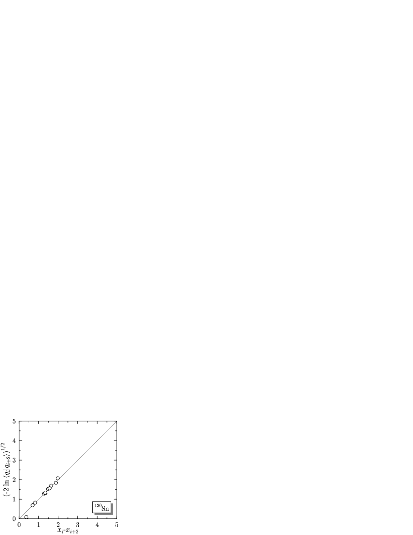
Figure 7: Overlaps of angular-momentum and particle-number projected states from second-nearest neighbor configurations of ¹²⁰Sn. The ordinate and abscissa indicate the actual and the GOA-estimated overlaps, respectively.

Unexpectedly large overlaps between prolate and oblate projected states were also found in the previously mentioned study of the interacting boson model ha03 . In fact it is easy to understand this behavior. For small deformations, the intrinsic configuration may be expanded as $|q\rangle\approx|0\rangle+\alpha Q^{\dagger}|0\rangle+\alpha^{2}Q^{\dagger}Q^{\dagger}|0\rangle/2+\ldots$ where $Q$ is a particle-hole operator transforming as $J=2$, $M=0$ under rotations and $\alpha$ is a deformation parameter. On projection, the wave function becomes $P_{J=0}|q\rangle\approx|0\rangle+\alpha^{2}/2\sqrt{5}(Q^{\dagger}Q^{\dagger})^{0}|0\rangle+\ldots$. This wave function does not depend on the sign of $\alpha$. Thus, the same state can be obtained by projecting a prolate or an oblate intrinsic state.

This behavior is also found for crossover matrix elements between more highly deformed configurations, and it prevents us from defining a linear metric $x$ to estimate the crossover matrix elements. A possible procedure could be to carefully select the sequence of deformations so that eq. (11) is not applied to estimate high-overlap crossover matrix elements. This strategy is illustrated in Fig. 8. The dashed line shows the path for a naive scheme for assigning a distance between configurations.

Figure 8: Linear metrics for GOA mixing prolate and oblate shapes. The naive metric is defined by the path passing through the spherical point, shown by the dashed line in the figure. An improved metric bypasses the spherical point via the path AB.

The points marked $A$ and $B$ would be separated by a distance $\Delta x$ given by the sum of the distances between the origin and those two points. But from what we said before, the angular-momentum projected configurations $A$ and $B$ would actually have a very high overlap, larger than with the spherical configuration. Modifying the path by taking the short-cut $AB$ (dotted line), the overlap $I_{0}(q_{A},q_{B})$ will be determined exactly and the errors for more distant crossover overlaps will be reduced. This procedure offers an improvement, but more distance crossover overlaps such as $AC$ are still underestimated. This suggests that the two-dimensional geometry of Fig. 8 might be used to define a better metric for the overlaps: measure the distance along the lines for the prolate and oblate configurations separately as done before, but use the triangular geometry of Fig. 8 to determine crossover overlaps. We put the prolate configurations along the horizontal axis, and write their position as a vector $\vec{x}_{i}=(x_{i},0)$. The oblate configurations are put on a line making an angle $\alpha$ with respect to the horizontal axis, located at positions $\vec{x}_{i}=x_{i}(\cos\alpha,\sin\alpha)$. The distance between configurations $q_{i},q_{j}$ is taken to be $y_{ij}=|\vec{x}_{i}-\vec{x}_{j}|$, which is to be applied in general without distinguishing prolate and oblate. We will call this the triangular GOA, and will apply it below. In general, the angle $\angle A0B$ of the triangle depends on the distances, becoming more acute the closer $A$ and $B$ are to the spherical point. For the configuration sets used here, the spacings are such that the angles range from $30^{\circ}$ to $60^{\circ}$. In the application below, we assume a fixed angle of $45^{\circ}$.

We now turn to the estimation of the Hamiltonian matrix element. The first step for a GOA estimate is to express the matrix element as a product of the overlap and a smoothly varying factor $h(q_{i},q_{j})$,

$$\langle q_{i}|H|q_{j}\rangle=h(q_{i},q_{j})I_{0}(q_{i},q_{j}).$$

The factor $h$ is expanded as a power series in $|\vec{x}_{i}-\vec{x}_{j}|$,

$$h(q_{i},q_{j})=h_{0}(\bar{x})-h_{2}(\bar{x})|\vec{x}_{i}-\vec{x}_{j}|^{2},$$ (12)

where $\bar{x}=(x_{i}+x_{j})/2$. This equation will be used to define $h_{2}$ between nearest-neighbor configurations $q_{i},q_{i+1}$, taking the computed Hamiltonian matrix element as input. To assign nearest neighbors, we drop the spherical point and use the dotted path shown in Fig. 8. The definition of $h_{2}$ on these links is thus

$$h_{2}(i,i+1) = \frac{1}{|\vec{x}_{i}-\vec{x}_{i+1}|^{2}}\bigg{(}\frac{h(q_{i},q_{i})+h(q_{i+1},q_{i+1})}{2}$$

$$-h(q_{i},q_{i+1})\bigg{)}.$$

We average the $h_{2}$ on the links between two states to get an estimated $\bar{h}_{2}$ to use in their matrix element. Then the matrix element of the Hamiltonian on the $J-$projected states is estimated as

$$h(q_{i},q_{j})=\frac{1}{2}\big{[}h(q_{i},q_{i})+h(q_{j},q_{j})\big{]}+\bar{h}_{2}\,|\vec{x}_{i}-\vec{x}_{j}|^{2}.$$ (13)

We now have complete matrices both for the overlap and the Hamiltonian and it is diagonalized exactly the same way as in the full theory. This is usually done by first diagonalizing the matrix of overlaps $I_{0}$ and constructing its square root. Then the matrix

$$I_{0}^{-1/2}HI_{0}^{-1/2}$$

is then diagonalized, and its eigenvalues give the energies of the GCM theory. We remind the reader that the method has numerical instabilities if the configurations are too close. This is circumvented by truncating the basis, removing states whose norm is small (typically $\leq 0.01$). In such situations, there is a sensitivity to elements of the norm matrix that are quite removed from the main diagonal. It is for this reason that the GOA needs to be rather accurate. As an example, the configuration set used to represent ¹²⁰Sn, three of the thirteen eigenstates of the norm matrix had eigenvalues less that $0.01$ and were discarded.

We now compute the correlation energy for a sample of nuclei using the triangular GOA and compare with the results of the fully calculated matrices. The resulting configurational correlation energy eq. (9) is displayed in Fig. 9. The horizontal axis shows the value in the GOA using eqs. (11) and (13), and the vertical axis shows the accurate result of the full calculation.

Figure 9: Comparison of configurational correlation energies $\Delta E_{HW}$, eq. (9), computed with the triangular GOA to the numerically accurate values.

The errors using the estimated matrix elements are all within the targeted accuracy of $\pm 0.2$ MeV. We conclude that the procedure has sufficient accuracy to be used in a first survey of the nuclear mass table.

For numerical purposes in general, it is also important to know how close together the configurations need to be to get reliable energies. Ref. bo90 indicates that $\delta x=1.6$ (overlap of 30%) is adequate and $\delta x=1.1$ (overlap of 55%) is safe, taking a criterium of 0.2 MeV for energy convergence. This seems to be valid for the $J-$projected configurations as well. For example, for the nucleus ¹²⁰Sn, we can thin the configuration set taking out states whose overlaps with neighbors exceeds 55%. Here the thinned space has only 4 configurations, compared with 13 in the original set. The configurational correlation energy is nearly unchanged by the thinning and is within the desired error bound. Clearly, more study is needed to find an optimum spacing for a global prescription.

IV Examples of correlation energies

In this section we survey the trends of the correlation energy taking the results for a number of nuclei. In this sampling we have chosen nuclei to represent different kinds of structure in the mean field approximation, including closed-shell magic (²⁰⁸Pb), strongly deformed (¹⁵⁶Sm), and semi-magic with strong pairing (¹²⁰Sn). In addition, we consider two isotope chains, krypton and lead, which exhibit coexisting oblate and prolate deformations. The results are presented in Table 1. The first three columns of energies show the numerically converged correlation energies obtained with the $N$, $Z$, and $J$ projections and Hill-Wheeler representation as in refs. va00 ; du03 ; BFH03 ; be03 .

The first column gives $\Delta E_{corr}$, the energy gain over that of the lowest intrinsic configuration associated with angular momentum projection, defined in eq. (7). We should note that we only use the given configurations to determine the energy minimum for the projected states, $\min_{q}E_{qq,J=0}$, which could give some error in assigning the energy gain. There will be a compensating error in the value of the configurational correlation energy, with the total independent of $\min_{q}E_{qq,J=0}$. In the table, the nuclei for which the deformation $q$ is significantly different for the intrinsic and the projected configurations are indicated with asterisks. An example where the deformation is virtually identical before and after projection is ¹⁵⁶Sm. Its correlation energy is 3.0 MeV, which is rather typical for deformed nuclei. What is surprising to us is that the other nuclei have rotational correlation energies of the same order of magnitude. The semi-magic “spherical” nucleus ¹²⁰Sn is a case in point. At the mean-field or intrinsic level, the ground state is indeed spherical, but the energy after angular momentum projection is lower for the configuration with $q=400$ fm². Qualitatively this behavior is to be expected, because the variation-after-projection is a way to introduce correlations from the attractive parts of the interaction that only have perturbative character. The surprising finding is the magnitude, which is only 10% lower in ¹²⁰Sn than the value for a fully deformed nucleus. In fact all the nuclei except the doubly-magic ²⁰⁸Pb have correlation energies in the same range.

Table 1: Correlation energies in the GCM associated with quadrupole deformations. Energies are given in MeV.

Z	A	$\Delta E_{corr}$	$\Delta E_{HW}$	total	GOA
36	74	2.9	0.8	3.7	3.7
36	78	2.4∗	0.9	3.3	3.2
36	82	3.0	0.8	3.8	3.5
36	86	2.8	0.4	3.3	3.0
50	120	2.8∗	0.8	3.6	3.3
62	156	3.0	0.8	3.8	3.8
82	186	2.7	0.9	3.6	3.3
82	190	2.7	1.0	3.8	3.7
82	194	2.8	1.1	3.9	3.7
82	208	1.5∗	0.2	1.7	1.6

The next column of the table shows additional energy gain obtained by solving the Hill-Wheeler equation to mix configurations, $\Delta E_{HW}$ in eq. (9). Except for the doubly-magic ²⁰⁸Pb, these numbers are remarkably constant over the nuclei considered, ranging in value from 0.8 to 1.1 MeV. The nucleus ²⁰⁸Pb behaves in a similar way as the model discussed in ref. ha03 . That model permitted a significant energy by projection, but the optimal projected state had a very high overlap with the true eigenstate, and there was no further energy gain by mixing configurations.

The third column shows the total correlation energy, $\Delta E_{corr}+\Delta E_{HW}$. The range of variation is 0.6 MeV, except for ²⁰⁸Pb.

The last column in Table 1 shows the total correlation energy computed with the approximations in the treatment of the Hill-Wheeler equation described in the last section. The results are very close to that of the full treatment, with the r.m.s. error having a value of 0.15 MeV. We now come to the conclusions that we draw from these results.

V Conclusions

Although the primary purpose of this study was numerical and we only examined a small sample of nuclei, our findings suggest the possible physics that may emerge from a systematic, global study of the quadrupolar correlation energy. One might naively expect that the energy of projection would be large for deformed nuclei but not for others. In fact we found that this energy is rather large except for the doubly magic nucleus that we considered. The additional energy associated with vibrations is small, less than one MeV, and not very different from one nucleus to another. For the sum we see fluctuations of the order a few hundred keV.

In the global theories of nuclear masses, one treats the mean-field effects in detail but up to now ignoring or approximating in a phenomenological way fluctuating parts of the correlation energy. The relative constancy of our calculated correlation energy suggests that these fluctuations are indeed small, permitting a mean-field treatment to be quite successful. On the other hand, the fluctuation effects we have found are large enough to be potentially useful. In the present mass theories there are r.m.s. deviations of the order of 700 keV. For the nine nuclei in Table 1, the r.m.s. fluctuation in the total correlation energy is 650 keV. This gives grounds for the hope that including the quadrupolar correlation energy in calculating nuclear masses might significantly improve the agreement with the experimental values and produce a theory with better predictive power.

On the numerical side, the GOA for angular momentum projection reduces the computational cost by almost an order of magnitude. A similar saving is realized by the triangular GOA for the Hill-Wheeler matrices, which only requires computing diagonal and next-to-diagonal elements. This brings the total cost down the same level as the HF+BCS computations of the GCM configurations, and makes feasible a systematic determination of correlation energies for the nuclear mass table.

We thus have the intention of continuing this project to compute the quadrupolar correlation energies of all even-even nuclei. For a global calculation we would need to use an energy functional that is applicable across the chart of nuclides. We have been using the SLy6 Skyrme parameterization, but so far the pairing parameters have been different for light and heavy nuclei. Ultimately, a new fit of the mean field energy functional will be required, but for a first survey of the correlation energy it should be sufficient to take the same functional, but with a fixed pairing interaction.

Acknowlegments

We wish to acknowledge helpful discussions with H. Flocard, P.-G. Reinhard, and K. Hagino. GFB acknowledges support by the US Department of Energy under Grant DE-FG-06-90ER40561, the Guggenheim Foundation, and the Institut de Physique Nucléaire d’Orsay. PHH thanks the Institute for Nuclear Theory in Seattle, where this work was initiated. This work has been partly supported by the PAI-P5-07 of the Belgian Office for Scientific Policy. MB acknowledges support through a European Community Marie Curie Fellowship.

Appendix: Summary of computational costs

Our aim is to reduce the computing time needed to calculate correlation energies at a level comparable to that of mean-field calculations. Let us estimate the cost of both and to determine how they scale with the number of nucleons. The parameters which govern the computing time are the number of active orbitals $N_{act}$ and the dimension of the vector representing an orbital $N_{r}$. The mesh size is always fixed to 0.8 fm, a value sufficient to have a satisfactory accuracy on energies. The number of mesh points must be large enough to guarantee that the wave functions can be set equal to zero at the edge of the box so that derivatives and the Coulomb boundary conditions can be calculated accurately. The mean-field equations are solved by the imaginary time method and one can limit the number of orbitals that have to be computed to the orbitals close to the Fermi level. In practical applications, to be on the safe side, $N_{act}$ and $N_{r}$ are chosen larger than required.

In Hartree-Fock theory $N_{act}$ is equal to $N_{occ}$, the number of occupied orbitals. Due to time-reversal symmetry, the orbitals are two-fold degenerate and the number of orbitals is half the number of nucleons. When pairing correlations are taken into account, either at the BCS or at the Bogoliubov level, $N_{act}$ is larger. In practical applications, to be sure that enough HF wave functions are computed, $N_{occ}$ is taken around $2A/3$.

Calculations are performed in a 3-dimensional coordinate grid representation. To calculate the nuclear ground state and to be able to easily rotate the orbital wave functions on the mesh, we consider only cubic meshes. In practice, the actual dimension of the grid can be reduced by symmetry considerations. The reflection symmetry of the mean-field Hamiltonian allows one to consider only the points in an octant. We will thus define $N_{x}$ to be the number of points along the positive $x$-axis. However, there is a price to pay for using this symmetry: the wave functions must be complex. Also, the spin degree of freedom doubles the size of the vector. In the end the dimension of a real array representing an orbital is

$$N_{r}=4N_{x}^{3}.$$

The number of points scale roughly as $3A^{1/3}$, although the number used in practical applications is larger for light nuclei. This dependence on $A$ ensures that the wave functions can be safely put to zero at the edge of the box.

The mean-field calculation is done iteratively, determining in each cycle the total energy of the nucleus, the HF Hamiltonian and its action on the individual wave functions. These computations need to be repeated a number of time equal to the total number of iterations required for a full convergence, typically 200 to 400 times. It has also to be done for each quadrupole moment which will enter the GCM calculation. The GCM requires calculating the overlaps and the Hamiltonian matrix elements between wave functions with different orientations and deformations. Let us first evaluate the computational effort that is required for a single set of Euler angles and a single deformation. This effort is similar to that required to calculate the energy in the mean-field calculation.

For the calculation of a matrix element of the GCM Hamiltonian kernel or the total HF energy the dominant terms are those with derivatives of the wave functions. This has a computational cost given by

$$6N_{act}N_{r}N_{x},$$ (14)

following the method of ref. ba86 . A prefactor 3 accounts for the three Cartesian directions along which derivatives have to be calculated. The prefactor 2 counts separately the multiplication of the initial vector and the addition to the final vector. Several terms in the Hamiltonian matrix element involve derivations, e.g. those associated with the spin-orbit field, and the total computational effort is an order of magnitude larger than given by the expression Eq. (14). More terms appear in the GCM calculation due to the presence of vector densities which are equal to zero for diagonal matrix elements.

The cost related to particle-number projection is not easy to evaluate, since this projection is intimately mixed with the other part of the calculation. We use the method of ref. HBD93 which requires one to multiply the $v$ factor of the Bogoliubov transformation by a phase. The calculation of the derivatives of the wave functions is not affected by this projection. However, all densities become complex.

The mean-field calculation requires one to calculate also the action of the HF Hamiltonian on all mean-field wave functions. Once more, the most time-consuming part concerns terms including derivatives. They are grouped in terms with first and second order derivatives acting on the four components of the wave functions, with 24 terms in total.

In the GCM case, another time-consuming task is rotating the many-particle wave function, an operation that is needed for angular momentum projection. This is done by interpolating the single-particle wave functions in the $x-z$ plane to the points corresponding to some rotation $\theta$ about the $y$-axis,

$$R_{\theta}:\,\,\,(x,z)=(x^{\prime}\rightarrow x\cos\theta+z\sin\theta,z^{\prime}\rightarrow-x\sin\theta+z\cos\theta).$$

The needed accuracy is achieved by using all the points in a half plane to interpolate in that plane. The computational cost here is

$$4N_{act}N_{r}N_{x}^{2}$$

where the factor 4 includes a factor 2 for expanding from a quarter-plane slice of the octant to the half plane.

To take overlaps, one needs to calculate a determinant. The determinant is of order $N_{act}$ and setting up its matrix requires

$$2N_{act}^{2}N_{r}$$

operations. Since $N_{r}$ is usually less than $N_{act}$, this is usually the most time consuming task. However, the simultaneous projection on particle number and angular momentum requires also additional calculations to follow the phase of the overlap kernel. Test calculations indicate that the particle number projection approximately doubles the computing of the determination of the GCM kernels.

For our calculations, $N_{x}$ is of the order of 14 (Kr) to 16 (Pb). Thus the vector size is about $N_{r}\approx 4*15^{3}=13,500.$ The number of orbitals for Pb is around $N_{act}=140$. With these numbers, the interpolation of the wave functions has about the same cost as setting up the determinants.

Putting all these numbers together with realistic values, one can estimate that the determination of a single point for the GCM+projection calculation takes a factor 10 longer than a single mean-field iteration.

The computing time is also determined by the number of times these basic calculations have to be done. It is the number of iterations (typically 300) times the number of quadrupole moments that have to be considered (typically 15) for the mean-field part. For the GCM part, it is the number of active Euler angles (typically 12) times the number of matrix elements (typically $15^{2}$). With all these numbers, the GCM calculation is an order of magnitude longer than the mean-field calculation. Reducing the number of Euler angles to 1 or 2 and the number of matrix elements to be determined exactly to 2 times the number of discretized quadrupole moments reduce this part of the calculation to a time similar to the mean-field calculation.

References

- (1) S. Goriely, M. Samyn, P.-H. Heenen, J. M. Pearson, F. Tondeur, Phys. Rev. C 66, 024326 (2002); M. Samyn, S. Goriely, and J. M. Pearson, Nucl. Phys. A725, 69 (2003); S. Goriely, M. Samyn, M. Bender, and J. M. Pearson, Phys. Rev. C, in print.
- (2) M. Bender, P.-H. Heenen and P.-G. Reinhard, Rev. Mod. Phys. 75, 121 (2003).
- (3) P. Bonche, J. Dobaczewski, H. Flocard, and P.-H. Heenen, Nucl. Phys. A530, 466 (1991).
- (4) P.-H. Heenen, P. Bonche, J. Dobaczewski and H. Flocard, Nucl. Phys. A561, 367 (1993).
- (5) J. Meyer, P. Bonche, M. S. Weiss, J. Dobaczewski, H. Flocard and P.-H. Heenen, Nucl. Phys. A588, 597 (1995).
- (6) P.-H. Heenen, A. Valor, M. Bender, P. Bonche and H. Flocard, Eur. Phys. J. A. 11, 393 (2001).
- (7) A. Valor, P.-H. Heenen, P. Bonche, Nucl. Phys. A671, 145 (2000).
- (8) M. Bender, P.-H. Heenen, Nucl. Phys. A713, 390 (2003).
- (9) T. Duguet, M. Bender, P. Bonche, and P.-H. Heenen, Phys. Lett. B559, 201 (2003); M. Bender, P. Bonche, T. Duguet, and P.-H. Heenen, to be submitted.
- (10) M. Bender, H. Flocard, and P.-H. Heenen, Phys. Rev. C 68 044321 (2003).
- (11) K. Hagino, P.-G. Reinhard, and G. F. Bertsch, Phys. Rev. C 65, 064320 (2002).
- (12) K. Kumar and M. Baranger, Nucl. Phys A122, 273 (1968).
- (13) M. Girod and B. Grammaticos, Nucl. Phys. A330, 40 (1979).
- (14) L. Prochniak, P. Quentin, D. Samsoen and J. Libert, Acta Phys. Pol. B34, 2461 (2003).
- (15) R. K. J. Sandor, H. P. Blok, M. Girod, M. N. Harakeh and C. W. de Jager, Nucl. Phys. A551, 349 (1993).
- (16) A. Góźdź, K. Pomorski, M. Brack and E. Werner, Nucl. Phys. A442, 26 (1985).
- (17) S. Pilat and K. Pomorski, Nucl. Phys. A554, 413 (1993).
- (18) L. Próchniak, K. Zaja̧c, K. Pomorski, S. G. Rohoziński and J. Srebrny, Nucl. Phys. A648, 181 (1999).
- (19) P. Bonche, J. Dobaczewski, H. Flocard, P.-H. Heenen, and J. Meyer, Nucl. Phys. A510, 466 (1990).
- (20) C. Rigollet, P. Bonche, H. Flocard, P.-H. Heenen, Phys. Rev. C 59, 3120 (1999).
- (21) D. Baye and P.-H. Heenen, J. Phys. A 19, 2041 (1986).
- (22) F. Villars and N. Rogenson, Ann. Phys. (NY) 63 443 (1971).
- (23) S. Islam, H. J. Mang, and P. Ring, Nucl. Phys. A326, 162 (1979).
- (24) D. Baye and P.-H. Heenen, Phys. Rev. C 29, 1056 (1984).
- (25) K. Hagino, G. F. Bertsch, and P.-G. Reinhard, Phys. Rev. C 68, 024306 (2003).