Three-body Thomas-Ehrman shifts of analog states of ¹⁷Ne and ¹⁷N

Abstract

The lowest-lying states of the Borromean nucleus ¹⁷Ne (¹⁵O+$p$+$p$) and its mirror nucleus ¹⁷N (¹⁵N+$n$+$n$) are compared by using the hyperspheric adiabatic expansion. Three-body resonances are computed by use of the complex scaling method. The measured size of ¹⁵O and the low-lying resonances of ¹⁶F (¹⁵O+$p$) are first used as constraints to determine both central and spin-dependent two-body interactions. The interaction obtained reproduces relatively accurately both experimental three-body spectra. The Thomas-Ehrman shifts, involving excitation energy differences, are computed and found to be less than 3% of the total Coulomb energy shift for all states.

I Introduction

Nuclear halos are expected along the driplines where nucleon single particle $s$ or $p$-states occur with sufficiently small separation energy han95 ; rii00 . A cluster description of the nucleus can then be appropriate, being able to visualize the nucleus as a system made by an ordinary nucleus (the core) surrounded by one or two nucleons. Since the Coulomb interaction works against halo formation the appearance of proton halos requires a relatively light core rii92 ; fed94 . Still the degrees of freedom describing the core and the surrounding protons may decouple and justify a few-body treatment.

The lightest Borromean proton dripline nucleus is ¹⁷Ne (¹⁵O$+p+p$) which has an odd core mass implying finite core spin. The low-energy properties of the two-body proton-core subsystems produce the two sets of known spin-split pairs of resonances gui98 . Dealing with the details of such systems is delicate but analogous to the proper treatment of ¹¹Li gar97 . Unfortunately the structure of ¹⁷Ne, even within three-body models, seems to be very controversial and differing rather strongly in available publications gri03 ; tim96 .

Nevertheless ¹⁷Ne was recently discussed gri02 as an example revealing new features of the Thomas-Ehrman shift ehr51 . This necessarily introduces the mirror nucleus with less Coulomb repulsion which then must be more bound and possibly with a different structure. In fact the basic assumptions of the three-body model could be violated. Still it is interesting to push model applications to test its limits. We shall therefore try to describe ¹⁷N with precisely the established model parameters and compare effects of the (lack of) Coulomb interactions.

The paper is organized as follows: In section II we describe very briefly the method used to compute three-body bound wave functions as well as three-body resonances. We continue in section III with the description of the nucleon-nucleon and nucleon-core interactions needed to study ¹⁷Ne and ¹⁷N. We then in section IV compare the properties of the low-lying states of these two mirror nuclei. In section V we discuss in details the three-body Thomas-Ehrman shifts for all these states. We close the paper with a summary and conclusions.

II Three-body method

The three-body wave functions are computed using the hyperspheric adiabatic expansion method fed94 ; nie01 , that solves the Faddeev equations in coordinate space. The wave function, $\Psi=\sum\psi_{i}$, is then written as a sum of three Faddeev components $\psi^{(i)}(\bm{x}_{i},\bm{y}_{i})$ ($i$=1,2,3), where $\{\bm{x}_{i},\bm{y}_{i}\}$ are the three sets of Jacobi coordinates defined for instance in fed94 . We then introduce the hyperspheric coordinates, ($\rho=\sqrt{x^{2}+y^{2}}$, $\alpha_{i}=\arctan({x_{i}/y_{i}})$, $\Omega_{x_{i}}$, and $\Omega_{y_{i}}$), and for each value of $\rho$ we expand each component $\psi^{(i)}$ in terms of a complete set of angular functions:

$$\psi^{(i)}=\frac{1}{\rho^{5/2}}\sum_{n}f_{n}(\rho)\phi_{n}^{(i)}(\rho,\Omega_{i});(\Omega_{i}\equiv\{\alpha_{i},\Omega_{x_{i}},\Omega_{y_{i}}\}),$$ (1)

When this expansion is introduced in the Faddeev equations they can be separated into an angular and a radial part. The angular part takes the form

$$\hat{\Lambda}^{2}\phi_{n}^{(i)}+\frac{2m\rho^{2}}{\hbar^{2}}V_{jk}(x_{i})\left(\phi_{n}^{(i)}+\phi_{n}^{(j)}+\phi_{n}^{(k)}\right)=\lambda_{n}(\rho)\phi_{n}^{(i)}$$ (2)

where $V_{jk}$ is the two-body interaction between particles $j$ and $k$, $\hat{\Lambda}^{2}$ is an angular operator nie01 and $m$ is the normalization mass. The complete set of angular functions used in (1) are the eigenvectors of the angular part of the Faddeev equations, that are labeled with the index $n$ and whose eigenvalues are denoted by $\lambda_{n}(\rho)$.

Finally, the coefficients $f_{n}(\rho)$ in the expansion (1) are obtained after solving the coupled set of equations given by the radial parts of the Faddeev equations:

$$\left[-\frac{d^{2}}{d\rho^{2}}+\frac{2m}{\hbar^{2}}(V_{3b}(\rho)-E)+\frac{1}{\rho^{2}}\left(\lambda_{n}(\rho)+\frac{15}{4}\right)\right]f_{n}(\rho)$$

$$+\sum_{n^{\prime}}\left(-2P_{nn^{\prime}}\frac{d}{d\rho}-Q_{nn^{\prime}}\right)f_{n^{\prime}}(\rho)=0\;\;\;\;$$ (3)

where $V_{3b}$ is a three-body potential used for fine-tuning and the functions $P_{nn^{\prime}}$ and $Q_{nn^{\prime}}$ can be found for instance in nie01 . The eigenvalues $\lambda_{n}(\rho)$ are essential in the diagonal part of the effective radial potentials:

$$V_{\mbox{eff}}(\rho)=\frac{\hbar^{2}}{2m}\frac{\lambda_{n}(\rho)+15/4}{\rho^{2}}+V_{3b}(\rho)$$ (4)

The hyperspheric adiabatic expansion method was initially designed to compute three-body bound state wave functions, and therefore the coupled set of radial equations (3) was solved for radial solutions falling off exponentially at large distances. In principle the method can also be used to calculate continuum and resonance wave functions. Then we must require the correct asymptotic behaviour for the solutions to eqs.(3) as described in cob97 .

Calculations of resonance wave functions are in practice significantly simplified by using the complex scaling method fed03 where the radial coordinates are rotated into the complex plane by an arbitrary angle $\theta$. This transformation of the Jacobi coordinates ($x\rightarrow xe^{i\theta}$, $y\rightarrow ye^{i\theta}$) implies that only the hyperradius $\rho$ is transformed ($\rho\rightarrow\rho e^{i\theta}$), while the hyperangles remain unchanged. It is then known that as soon as the scaling angle $\theta$ is larger than the argument of the resonance, then the complex rotated resonance wave function falls off exponentially, exactly as a bound state. Therefore, after complex scaling, the resonances can be computed with the same numerical techniques as for bound states.

III Two-body potentials

In this section we investigate the two-body potentials needed to compute the three-body system ¹⁷Ne (¹⁵O+$p$+$p$). The short-range interaction for the mirror nucleus ¹⁷N (¹⁵N+$n$+$n$) is then in principle the same although the assumptions of the three-body model are much less convincing due to the larger binding energy. The spin-dependence of the effective two-body interactions must be carefully chosen as shown in gar03 . For symmetry reasons the spin-spin and spin-orbit operators in the nucleon-nucleon interaction should be $\bm{s}_{1}\cdot\bm{s}_{2}$ and $\bm{\ell}\cdot(\bm{s}_{1}+\bm{s}_{2})$, respectively, where $\bm{s}_{1}$ and $\bm{s}_{2}$ are the spins of the two nucleons and $\bm{\ell}$ is their relative orbital angular momentum.

For the nucleon-core interaction it is necessary to introduce operators that conserve the usual mean field quantum numbers, i.e. the nucleon total angular momentum $\bm{j}_{n}=\bm{\ell}+\bm{s}_{n}$ and the total two-body angular momentum $\bm{j}=\bm{j}_{n}+\bm{s}_{c}$, where $\bm{\ell}$ now is the relative nucleon-core orbital angular momentum, and $\bm{s}_{c}$ and $\bm{s}_{n}$ are the core and nucleon spin, respectively. This almost uniquely determines the spin operators as the usual fine and hyperfine terms $\bm{\ell}\cdot\bm{s}_{n}$ and $\bm{s}_{c}\cdot\bm{j}_{n}$ gar03 .

III.1 Nucleon-nucleon interaction

For the nucleon-nucleon short-range interaction we use the operators mentioned above, and in particular the potential given in gar97

$$V_{NN}(r)=37.05e^{-(r/1.31)^{2}}-7.38e^{-(r/1.84)^{2}}$$

$$-23.77e^{-(r/1.45)^{2}}{\bm{\ell}\cdot\bm{s}}+7.16e^{-(r/2.43)^{2}}S_{12}$$

$$+\left(49.40e^{-(r/1.31)^{2}}+29.53e^{-(r/1.84)^{2}}\right){\bm{s}}_{1}\cdot{\bm{s}}_{2}+\frac{(eZ_{n})^{2}}{r}\;$$

where $\bm{s}=\bm{s}_{1}+\bm{s}_{2}$ and $S_{12}$ is the usual tensor operator, $e$ is the unit electric charge and $Z_{n}(=0,1)$ is the nucleon charge number. The strengths are given in MeV and the ranges in fm. This potential reproduces the experimental scattering lengths and effective ranges of the ${}^{1}S_{0}$, ${}^{3}P_{0}$, ${}^{3}P_{1}$, and ${}^{3}P_{2}$ waves. We use the same interaction for relative orbital angular momenta larger than 1.

III.2 Nucleon-core interaction

For the nucleon-core interaction we construct an $\ell$-dependent potential of the form:

$$V^{(\ell)}_{N-core}(r)=S_{c}^{(\ell)}f^{(\ell)}_{c}(r) + S_{ss}^{(\ell)}f^{(\ell)}_{ss}(r)\bm{s}_{c}\cdot\bm{j}_{n}$$

$$-S_{so}^{(\ell)}\frac{1}{r}\frac{d}{dr}f^{(\ell)}_{so}(r)\bm{\ell}\cdot\bm{s}_{n} + \frac{Z_{c}Z_{n}e^{2}}{r}{\rm Erf}(r/b_{c})\;,$$ (6)

where $\bm{s}_{n}$ and $\bm{s}_{c}$ are the spin of the nucleon and the core, respectively, $\bm{\ell}$ is the relative orbital angular momentum between the two particles, $\bm{j}_{n}=\bm{\ell}+\bm{s}_{n}$, and $Z_{c}$ is the proton number of the core. The error function ${\rm Erf}$ describes the nucleon-core Coulomb interaction of a gaussian core-charge distribution where $b_{c}=2.16$ fm is fitted to reproduce a rms charge radius in ¹⁵O of 2.65 fm. This value is obtained from the measured rms charge radius in ¹⁶O (2.71 fm vri87 ) by rescaling it by an $A^{1/3}$ factor.

As discussed in gar03 the choice of these spin operators permits a clear energy separation of the usual mean-field spin-orbit partners $\ell_{\ell+1/2}$ and $\ell_{\ell-1/2}$. In this way it is possible to use a nucleon-core interaction such that the low-lying states have well defined $\ell_{j_{n}}$ quantum numbers, like the $p_{1/2}$ states in ¹⁰Li or $d_{5/2}$ states in ¹⁶F. The use of the $\bm{s}_{c}\cdot\bm{s}_{n}$ spin-spin and $\bm{\ell}\cdot(\bm{s}_{c}+\bm{s}_{n})$ spin-orbit operators makes this impossible, since then $j_{n}$ is not a conserved quantum number and the states in the two-body system are necessarily mixtures of $\ell_{\ell+1/2}$ and $\ell_{\ell-1/2}$ components. This is especially problematic in the case that one of these states is forbidden by the Pauli principle, like for instance the $p_{3/2}$ waves in ¹⁰Li.

The shapes of the central ($f^{(\ell)}_{c}$), spin-spin ($f^{(\ell)}_{ss}$) and spin-orbit ($f^{(\ell)}_{so}$) radial potentials in eq.(6) are chosen to be Woods-Saxon functions, $1/(1+\exp{((r-b_{\ell})/a)})$, with the same diffuseness $a$ in all cases. Once the range $b_{\ell}$ of each radial potential is chosen, the strengths $S_{c}^{(\ell)}$, $S_{ss}^{(\ell)}$ and $S_{so}^{(\ell)}$ are adjusted to reproduce the experimental spectrum of ¹⁶N (¹⁵N$+n$). For $s$-waves the strengths $S^{(0)}_{c}$ and $S^{(0)}_{ss}$ are used to fit the energies of the $s_{1/2}^{(j=0)}$ and the $s_{1/2}^{(j=1)}$ states (0^- and 1^- states). For $d$-waves the strength $S^{(2)}_{so}$ provides an appropriate spin-orbit splitting of the $d_{3/2}$ and the $d_{5/2}$ states while $S^{(2)}_{c}$ and $S^{(2)}_{ss}$ are used to reproduce the experimental binding energies of the $d_{5/2}^{(j=2)}$ and the $d_{5/2}^{(j=3)}$ states (2^- and 3^- states).

The role of the spin-orbit interaction is here only to place the $d_{3/2}$-states relatively high (they must remain unbound), and the precise energy of these states is not very relevant. In any case a appropriate estimation of the strength for the spin-orbit interaction requires knowledge of the $d_{3/2}^{(j=1)}$ and $d_{3/2}^{(j=2)}$ energies. In ¹⁶N there are two unbound 1^-/2^- doublets that could correspond to these states. Their experimental decay energies ajz86 (1.90 MeV and 2.58 MeV, or 2.27 MeV and 2.86 MeV) are used to estimate the strength of the spin-orbit interaction for $d$-waves.

Table 1: Range ($b_{\ell}$) and strengths of the central ($S_{s}^{(\ell)}$), spin-spin ($S_{ss}^{(\ell)}$), and spin-orbit ($S_{so}^{(\ell)}$) potentials in eq.(6). The diffuseness $a$ is 0.65 fm in all the cases.

$\ell$	$b_{\ell}$ (fm)	$S_{c}^{(\ell)}$ (MeV)	$S_{ss}^{(\ell)}$ (MeV)	$S_{so}^{(\ell)}$ (MeV$\cdot$fm2)
$0$	3.00	$-53.91$	0.92	–
$1$	2.70	$-19.99$	0.69	$-25.0$
$1$	2.92	$-54.15$	0.35	$-25.0$
$2$	2.85	$-58.45$	0.24	$-25.0$

The value of the range parameter $b_{\ell}$ is determined by the fact that by switching on the Coulomb potential the experimental spectrum of ¹⁶F (¹⁵O$+p$) should be reproduced. In table 1 we give the resulting values of the parameters used for the Woods-Saxon radial form factors in eq.(6). The partial waves with $\ell=0$ and $\ell=2$ are by far the most important in the present context.

The $s$-wave potential has a deeply bound state at $-31.0$ MeV in ¹⁶N and at $-26.2$ MeV in ¹⁶F. These states correspond to the $s_{1/2}$ nucleon states occupied in the ¹⁵N or the ¹⁵O core. They are then forbidden by the Pauli principle, and should be excluded from the calculation. This is implemented as in refs.gar97 ; gar99 by use of the phase equivalent potential which has exactly the same phase shifts as the initial two-body interaction for all energies, but the Pauli forbidden bound state is removed from the two-body spectrum. We then use the phase equivalent potential of the central part of the Woods-Saxon $s$-wave potential in table 1. Thus the $s$-states actively entering the three-body calculations are the second states of the Woods-Saxon potential. For the $d$-states no Pauli exclusion is necessary.

Table 2: Four lowest states in ¹⁶N and ¹⁶F obtained with the nuclear potential specified in table 1. For ¹⁶F we give the energies and widths of the two-body resonances $(E_{R},\Gamma)$. The experimental data are from ajz86 . Error bars are not specified when they are smaller than the last digit. For unbound states the energies are decay energies above threshold.

$J^{\pi}$	16N	Exp.	16F	Exp.
0-	$-2.37$	$-2.371$	(0.53,0.02)	(0.535, $0.040\pm 0.020$)
1-	$-2.09$	$-2.094$	(0.71,0.07)	($0.728\pm 0.006$, $<0.040$)
2-	$-2.49$	$-2.491$	(0.96,0.01)	($0.959\pm 0.005$, $0.040\pm 0.030$)
3-	$-2.19$	$-2.193$	(1.23,0.01)	($1.256\pm 0.004$, $<0.015$)

The bound states in ¹⁶N and low-lying resonances in ¹⁶F with $J^{\pi}$=0^-, 1^-, 2^-, 3^- are all obtained by coupling $s_{1/2}$ and $d_{5/2}$ with the core-spin of $1/2$. The calculated results are in table 2 compared with the experimental data for these states. The procedure of fitting the nuclear potential to reproduce simultaneously both the ¹⁶N and the ¹⁶F spectra is apparently efficient as the data is rather nicely reproduced. In fact this is not possible with other values for $b_{\ell}$.

In table 1 we also specify a $p$-wave interaction although these partial waves are expected to have only insignificant effects. The reason is that the lowest $p$-shell is fully occupied in the core and the unoccupied $p_{3/2}$ orbit is above the $d_{3/2}$-states and even higher than the $f_{7/2}$. Nevertheless, since the calculation will include $p$-wave components at least an estimate of the parameters for the corresponding interaction is desirable. We do this by using the knowledge of the unbound $1^{+}$ and $2^{+}$ states in ¹⁶N immediately above the bound $1^{-}$ state (with experimental decay energies 0.86 MeV and 1.03 MeV ajz86 , respectively). These resonances must arise from the coupling of a $p_{3/2}$ neutron with the spin 1/2 of the core (an $f_{7/2}$ neutron can not couple to 1 or 2) or perhaps by core excitation of a $p_{1/2}$ neutron. Again the potential parameters must be such that after switching on the Coulomb interaction the experimental decay energy of 4.30 MeV for the $1^{+}$ state in ¹⁶F has to be also reproduced (the experimental decay energy of the $2^{+}$ state of ¹⁶F is not available). The parameters fulfilling these conditions are given in the second line of table 1. The value of $S_{so}^{(1)}$ has been arbitrarily chosen to be the same as for $d$-waves.

The lowest $p$ shell is fully occupied in the ¹⁵N or ¹⁵O core. We should then apply the same treatment as for $s$-waves to the $p$-wave nucleon-core interaction, using a potential with deeply bound states that are afterwards removed by the corresponding phase equivalent potentials. For consistency we also tested a deep $p$-wave potential as given in table 1 with range and strengths comparable to the $s$ and $d$ potentials. The bound states in these deep $s$ and $p$ potentials produce a charge distribution with a rms radius in ¹⁵O of 2.63 fm consistent with the value used in the Coulomb potential. Furthermore the binding energies of the $p_{1/2}$ and $p_{3/2}$ states in ¹⁵O are $-7.29$ MeV and $-11.3$ MeV, respectively, both consistent with the experimental data ajz91 .

Nevertheless, since the $p$ waves basically have no effects in the three-body calculation we use for simplification the shallow $\ell$=1 potential given in table 1 without bound states. In this way the computing time is significantly reduced without loss in the computations accuracy.

IV Results for ¹⁷Ne and ¹⁷N

We use the two-body interactions determined as described in the previous section. The low-lying nucleon-core valence space is expected to consist of $s$ and $d$ waves. With spin and parity of $1/2^{-}$ for the core and two identical nucleons in the $sd$ valence space we can construct total angular momentum and parity states with $J^{\pi}$=1/2^-, 3/2^-, 5/2^-, 7/2^-, and 9/2^-. The next shells ($f_{7/2}$, $p_{3/2}$, $\cdots$ ) may also contribute but significant amounts of such components also indicate similar contributions from core excitations. These structures involve particle-hole excitations either from the $sd$ to the $pf$-shell or from the $p$ to the $sd$-shell. We shall neglect these core excitations.

IV.1 Components

To solve the eigenvalue problem given in eq.(2) we expand the angular eigenvectors in the basis $\{{\cal Y}_{\ell_{x}\ell_{y},L}^{K}(\alpha_{i},\Omega_{x_{i}},\Omega_{y_{i}})\otimes\chi_{s_{x}s_{y},S}\}$, where ${\cal Y}_{\ell_{x}\ell_{y},L}^{K}$ are the hyperspheric harmonics and $\chi$ is the spin function nie01 . For each of the three Jacobi coordinate sets $i$ the coordinate $\bm{x}_{i}$ is the vector connecting particles $j$ and $k$, the quantum number $\ell_{x}$ is the relative orbital angular momentum of particles $j$ and $k$, $\ell_{y}$ is the relative orbital angular momentum of particle $i$ and the center of mass of the $jk$ two-body system. The spin $s_{x}$ is the coupled spin of particles $j$ and $k$, and $s_{y}$ is the spin of particle $i$. Finally $L$ and $S$ are the coupling of $\ell_{x}$ and $\ell_{y}$, and of $s_{x}$ and $s_{y}$, respectively, and they couple to the total angular momentum $J$ of the system. The hypermomentum $K$ is given by $2n+\ell_{x}+\ell_{y}$ where $n$ is a non-negative integer counting the number of nodes in the Jacobi polynomials.

The first step in the calculation is then to choose the components to be included in the expansion of the angular eigenvectors. By direct but extensive computations, we have found that the components needed for ¹⁷Ne are essentially $s$, $p$, and $d$-waves. Only for high angular momentum ($J$=7/2 and 9/2) higher partial waves can be relevant. We then use the same components for ¹⁷N.

After solving the angular part of the Faddeev equations (2) we extract the angular eigenvalues $\lambda_{n}(\rho)$, that determine almost entirely the effective potentials entering in the radial equations (3). For both ¹⁷Ne and ¹⁷N we also here maintain the same number of lowest-lying adiabatic potentials for use in the radial equations (3). We compute first the bound state solutions falling off exponentially at large distances. Then the resonance eigenfunctions are found in complete analogy as exponentially falling solutions to the similar equations obtained by complex rotation of the hyperradius.

IV.2 Spectrum of ¹⁷Ne

We show the results in fig.1 for the four deepest effective potentials for the $1/2^{-}$, $3/2^{-}$, $5/2^{-}$, $7/2^{-}$, and $9/2^{-}$ states in ¹⁷Ne. It is known that at $\rho$=0 the values of the $\lambda$’s must reproduce the hyperspherical spectrum, $K$($K$+4) nie01 . In our case of positive total parity in the valence space $K$ must be even, i.e. $K$=0,2,4,$\cdots$.

Figure 1: The four lowest angular eigenvalues $\lambda_{n}(\rho)$ for the $1/2^{-}$, $3/2^{-}$, $5/2^{-}$, $7/2^{-}$ and $9/2^{-}$ states of ¹⁷Ne as function of $\rho$ where the normalization mass $m$ equals the nucleon mass.

In the figure we observe that the $\lambda$ function starting at zero ($K$=0) does not appear. This is due to the phase equivalent $s$-wave potential between proton and core where the deepest state of the initial potential is removed to account for the Pauli principle gar99 . By using the initial deep two-body potential instead we obtain a $\lambda$ function starting at zero for $\rho=0$ and diverging to $-\infty$ at large distances. This behaviour of the lowest $\lambda$ characterizes the existence of a bound two-body state nie01 . This state is actually the Pauli forbidden state which could have been computed and then omitted from the basis. Instead we suppressed the Pauli forbidden state by using the more consistent procedure with the phase equivalent potential.

For short-range potentials it is also known that at infinity the values of the $\lambda$’s must again follow the hyperspherical spectrum nie01 . However, this behaviour is changed for eigenvalues corresponding to unbound two-body states as soon as long-range interactions like the Coulomb potential are present. The reason is that the influence of the short-range interactions then disappear outside $\rho$-values corresponding to a few times the range of the interaction whereas the Coulomb potentials multiplied by $\rho^{2}$ give rise to linearly increasing $\lambda$ functions even at asymptotically large distances fed96 . This linear increase must appear as soon as only the Coulomb potential has an influence. The slopes depend on the geometric structure of the three-body system as the size increases.

The ground state of ¹⁷Ne is bound, and has a two-proton separation energy of $-944$ keV. The structure is about equal amounts of proton-core $s^{2}$ and $d^{2}$-waves. The computed root mean square radius is 2.8 fm consistent with the experimental value of $2.75\pm 0.07$ fm oza94 . All the excited states are unbound and computed by application of the complex scaling method. The excitation energies of the two lowest excited states are 1288$\pm$8 keV for the $3/2^{-}$ state and 1764$\pm$12 keV for the $5/2^{-}$ state gui98 . For both these states proton-core $s$-$d$ mixed components are dominating. In gui98 also a $7/2^{-}$ and a $9/2^{-}$ states are reported with excitation energies 2997$\pm$11 keV and 3548$\pm$20 keV, respectively. These four excitation energies correspond to the decay energies (energies above threshold) given in the second column of table 3. For these states the $d^{2}$-waves dominate. More details about the structure is available in gar03a .

The resonances obtained for ¹⁷Ne are extremely narrow with widths much smaller than the accuracy of our calculations. Thus, application of the complex scaling method allows the use of very small scaling angles. Typically complex scaling angles of $\theta$=10^-5 are able to find the ¹⁷Ne resonances. For these scaling angles the complex scaled $\lambda$’s can hardly be distinguished from the non-rotated functions in fig.1. The imaginary parts are very small and would appear on the zero line if plotted on the figure.

Table 3: The second and third columns give the experimental and computed bound state ($1/2^{-}$) and decay energies ($3/2^{-}$, $5/2^{-}$, $7/2^{-}$, and $9/2^{-}$) in ¹⁷Ne (in MeV). The fourth column are the strengths $S$ (in MeV) of the gaussian three-body forces that for a range of 4.0 fm give rise to energies matching the experimental values. The fifth column gives the expectation value of the three-body force for the corresponding ¹⁷Ne solutions. The last column is the contribution to the norm of the first three terms in the expansion (1).

$J^{\pi}$	$E_{exp}$	$E_{comp}$	$S$	$\langle V_{3b}\rangle$	$\lambda_{n=1,2,3}$ (%)
$1/2^{-}$	$-0.94$	$-0.79$	$-0.6$	$-0.2$	88.5, 11.1, 0.4
$3/2^{-}$	$0.34$	$0.63$	$-1.4$	$-0.3$	90.7, 8.9, 0.2
$5/2^{-}$	$0.82$	$0.91$	$-0.4$	$-0.1$	77.2, 16.9, 5.6
$7/2^{-}$	$2.05$	$2.24$	$-0.8$	$-0.2$	97.5, 2.3, 0.2
$9/2^{-}$	$2.60$	$2.70$	$-0.1$	$-0.1$	91.9, 4.2, 3.8

Using the $\lambda$ functions in fig.1 we obtain the ¹⁷Ne ground state binding energy and the decay energy of the excited states shown in the third column of table 3. As seen in the table the computed states are systematically less bound than the experimental value. This fact is actually expected, since three-body calculations using pure two-body interactions typically underbind the system. This problem is solved by inclusion of the weak effective three-body potential $V_{3b}$ in (3), that accounts for three-body polarization effects arising when the three particles all are close to each other. Therefore the three-body potential has to be of short range, while the three-body structure essentially is independent of the precise shape. This construction furthermore ensures that the two-body resonances remain unaffected within the three-body system after this necessary fine-tuning. The effective total potential entering is then given by (4).

The precise range of the three-body interaction also plays a limited role. This is because the three-body force is very weak compared to the depth of the full potential and furthermore it is largest for small $\rho$-values, where the total potential is highly repulsive. It is then clear that the main structure of the system can not be significantly modified by the choice of one or another of such three-body interactions. In table 3 we give the strengths of the gaussian three-body potentials which for range equal to 4 fm are needed to match the experimental energies of all these (ground and) excited states. One way to measure and compare the effect of the three-body force in the different calculations is to compute the expectation value $\langle V_{3b}(\rho)\rangle$ of the three-body potential for the corresponding $J^{\pi}$ solutions. In table 3 we also give this quantity which measures the contribution of the three-body force to the energy of the three-body system. A variation of the range of the three-body force within reasonable limits is not modifying the results.

In the last column of table 3 we give the contribution to the norm of the wave function of the first three terms in the expansion (1). Typically only two terms are enough to get an accuracy of 99%, and only for the $5/2^{-}$ and $9/2^{-}$ states the third term is giving a sizable contribution.

The spectrum of ¹⁷Ne has been previously investigated in gri03 ; tim96 . In both works the 3/2^- and 5/2^- levels are reversed compared to the experimental data, although in gri03 this deficiency is corrected by use of an appropriate three-body interaction. In the present work these problems are not encountered. When only the two-body forces describing properly the ¹⁶F spectrum are used, the ordering in the computed ¹⁷Ne spectrum is correct, as seen in the third column of table 3. Then, the use of a small effective three-body force is enough to fit the experimental data.

IV.3 Spectrum of ¹⁷N

Interchanging all neutrons and protons in ¹⁷Ne leads to the mirror system ¹⁷N which then analogously should be described as a three-body system with the ¹⁵N-core surrounded by two neutrons. The structure should then be obtained simply by switching off the Coulomb interaction for ¹⁷Ne, since the strong interaction is precisely the same due to charge symmetry. In this way we can compute the properties of ¹⁷N.

The results are listed in column two of table 4 and not surprisingly stronger binding is obtained. First, ¹⁷N is not a Borromean system. The number of three-body bound states has also increased substantially, i.e. we find two bound states both for $1/2^{-}$ and $3/2^{-}$, and one for $5/2^{-}$, $7/2^{-}$ and $9/2^{-}$. The computed energies of these states agree pretty well with the experimental values ajz86 . The discrepancy with the experiment is always smaller than 5%. Only for the excited $1/2^{-}$ and $3/2^{-}$ states a larger disagreement with the measured energies appears. In the third column of the table the calculations labeled by A+WS use the accurate Argonne nucleon-nucleon potential denoted in wir95 by $v_{18}$ and the Woods-Saxon nucleon-core potential in table 1.

Table 4: ¹⁷N spectrum obtained using the same nuclear two-body interactions as for ¹⁷Ne, and the effective three-body force given in table 3. The third column gives the results obtained with the Argonne (A) nucleon-nucleon potential plus the Woods-Saxon (WS) nucleon-core interaction (table 1). The last column gives the experimental data ajz86 .

$J^{\pi}$	$E$ (MeV)	$E_{\mbox{\scriptsize A+WS}}$ (MeV)	Exper.
$1/2^{-}$	$-8.54$	$-8.31$	$-8.374$
	$-3.72$	$-3.66$	$-4.711$
$3/2^{-}$	$-6.63$	$-6.80$	$-7.000$
	$-3.83$	$-5.03$	$-5.174$
$5/2^{-}$	$-6.32$	$-6.36$	$-6.467$
$7/2^{-}$	$-5.24$	$-5.17$	$-5.245$
$9/2^{-}$	$-4.58$	$-4.59$	$-4.745$

The relatively small differences between the mirror nuclei are perhaps not as self-evident if we consider the behavior of the angular eigenvalues shown in fig.2. We plot only the three lowest functions used to compute the different states in ¹⁷N. As for ¹⁷Ne there is no $\lambda$ function starting at zero due to the removal of the Pauli forbidden $s$-state by use of the phase equivalent potential. The main difference compared to fig.1 is the divergence towards $-\infty$ of all the $\lambda$ functions. This is a reflection of corresponding bound states in the two-body subsystems consistent with the quantum numbers of the three-body system. This underlines that ¹⁷N cannot be a Borromean nucleus nie01 . The qualitatively different behavior seen in figs.1 and 2 also emphasizes that the agreement with measurements for both nuclei is not a trivially build-in property of the present description. The model is consistent in a more profound way.

Figure 2: The three lowest effective potentials $\lambda_{n}(\rho)$ for the $1/2^{-}$ and $3/2^{-}$ (upper part), and $5/2^{-}$, $7/2^{-}$, and $9/2^{-}$ (lower part) states of ¹⁷N.

The spatial structure of ¹⁷N is less extended than that of ¹⁷Ne because its larger binding energy. The length scale as defined in jen03 is $\rho_{0}\approx 5.5$ fm ($\rho_{0}\approx 5$ fm for ¹⁷Ne) and the dimensionless measures of size and binding energy are $\langle(\rho/\rho_{0})^{2}\rangle\approx 0.9$ and $mB\rho_{0}^{2}/\hbar^{2}\approx 6.0$. The ground state of ¹⁷N is located in the same region as ordinary nuclei. Among the excited states shown in table 4 the less bound is the second $1/2^{-}$ state. For this state the corresponding dimensionless size and binding are 1.9 and 3.4, respectively, still located in the region of ordinary nuclei. The three-body structure is further illustrated in fig.3, where we show the square of the three-body wave function integrated over the directions of the Jacobi coordinates and multiplied by the volume element. The structure resembles that of ¹⁷Ne with two similar dominating peaks.

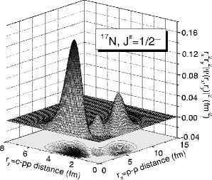
Figure 3: Contour diagram for the probability distribution of the $1/2^{-}$ ground state of ¹⁷N. The square of the three-body wave function is integrated over the directions of the two Jacobi coordinates.

The known properties of ¹⁷N seem to be rather well reproduced with the model parameters for ¹⁷Ne. An additional very small retuning of the strength of the effective three-body interaction could fit the lowest of each $J^{\pi}$ states. However, this would not improve the agreement of the second $1/2^{-}$ and $3/2^{-}$ states which then move into the positions $-3.62$ MeV and $-4.14$ MeV, respectively. This is probably because other effects are important, e.g. different components could now contribute both from valence space and from excitations. This is equivalent to an attempt to describe higher-lying resonances in ¹⁷Ne. They may also require another and perhaps enlarged Hilbert space. Further investigations of these well bound excited states are beyond the scope of the present report.

V Thomas-Ehrman shifts

The only difference in the computations of the two mirror nuclei is omission of the Coulomb interaction for ¹⁷N. This similarity is assumed inherently to describe the fundamental charge symmetry of the strong interaction. The immediate implication is that the differences in the spectra entirely must be produced by the Coulomb potential. The obvious difference is the shift of all energies towards stronger binding when the Coulomb potential is suppressed. However, this trivial overall shift is accompanied by a modified structure of the states. This is especially seen for the $s$-wave components which are less influenced by centrifugal barrier effects. The Coulomb repulsion tends to increase the size of a given state simply by minimizing the energy. The $s$-waves are here more influenced than higher partial waves and the shifts are then larger. This double difference in energy (excitation energy difference) is for single-particle energies called the Thomas-Ehrman shift ehr51 . It is due to the Coulomb interaction but not necessarily in a straightforward way. In a recent work gri02 the Thomas-Ehrman shift was investigated in the three-body systems ¹²O and ¹⁶Ne.

Table 5: The first column indicates the different states and calculations performed. The initials refer to the nucleon-nucleon+nucleon-core interactions used (G: Gaussian, WS: Woods-Saxon, A: Argonne). The second column gives the measured excitation energies of low-lying states in ¹⁷Ne. The computed ¹⁷Ne spectrum is identical. The measured and computed (¹⁷N)_th spectra in the mirror nucleus ¹⁷N are given in the third and fourth columns. The fifth and sixth columns contain the experimental ($\Delta_{e}$) and computed ($\Delta_{th}$) Thomas-Ehrman shifts. The seventh column shows the difference $\Delta_{e-th}$ between experimental and computed energies for ¹⁷N (see table 4). All the energies are given in MeV.

$\hskip 22.76219ptJ^{\pi}$	17Ne	17N	(17N)th	$\Delta_{e}$	$\Delta_{th}$	$\Delta_{e-th}$
$1/2^{-}$ G+WS	0.0	0.0	0.0	0.0	0.0	0.17
$1/2^{-}$ A+WS	”	”	”	”	”	$-0.06$
$3/2^{-}$ G+WS	1.29	1.37	1.91	0.08	0.62	$-0.37$
$3/2^{-}$ A+WS	”	”	1.51	”	0.22	$-0.20$
$5/2^{-}$ G+WS	1.76	1.91	2.22	0.15	0.46	$-0.15$
$5/2^{-}$ A+WS	”	”	1.95	”	0.19	$-0.11$
$7/2^{-}$ G+WS	3.00	3.13	3.30	0.13	0.30	$-0.01$
$7/2^{-}$ A+WS	”	”	3.14	”	0.14	$-0.08$
$9/2^{-}$ G+WS	3.55	3.63	3.96	0.08	0.41	$-0.17$
$9/2^{-}$ A+WS	”	”	3.72	”	0.17	$-0.16$

We compare in table 5 the spectrum of excitation energies for the two mirror nuclei. The second and third columns give the experimental excitation energies for the different states in ¹⁷Ne and ¹⁷N, respectively. The gaussian nucleon-nucleon interaction in eq.(III.1) and the Woods-Saxon nucleon-core potential in table 1 together with the three-body forces in table 3 reproduce the experimental ¹⁷Ne excitation energies. This calculation is denoted by G+WS. As in table 4 the calculation denoted by A+WS uses the Argonne nucleon-nucleon potential and the Woods-Saxon nucleon-core potential in table 1. A small three-body force also permits to reproduce the experimental ¹⁷Ne spectrum.

When these interactions are used for ¹⁷N the energies in table 4 and in the fourth column of table 5 are obtained. The computed excitation energies $(^{17}\mbox{N})_{th}$ of ¹⁷N are systematically higher than those measured. Still the agreement is surprisingly good in view of the fact that each state is computed independently by expansion on individual basis components without any parameter adjustment. This agreement is especially good for the A+WS calculation, where the short distance properties of the nucleon-nucleon interaction are carefully treated. Furthermore the states in ¹⁷N are well bound and the assumptions of independent degrees of freedom in the three-body cluster model cannot be very well fulfilled.

The experimental shifts ($\Delta_{e}$) are given in the fifth column of table 5. The total Coulomb shift (given by the energy difference between a ¹⁷Ne state and the corresponding ¹⁷N state) is of around 7.4 MeV. The values of $\Delta_{e}$ are then remarkably small compared to the 10% of the total Coulomb shift for the classical example of the single-particle $s$ and $d$-states in ¹⁷O and ¹⁷F. It is tempting to conjecture that this is due to the stronger effect of the centrifugal barrier in the three-body system where even the $s$-states feel a barrier. The Coulomb repulsion effect is then less pronounced than for a two-body system where the absence of the centrifugal barrier is the basic explanation.

The computed shifts ($\Delta_{th}$) are shown in the sixth column of the table. For the G+WS calculation they are clearly larger than the measured values, but also in these cases the computation represents an accuracy better than 10% of the Coulomb shift. In the A+WS computation $\Delta_{th}$ is no more than 3% of the Coulomb shift, and shows a better agreement with the experiment.

However, the $(^{17}\mbox{N})_{th}$ values given in the fourth column of table 5 are obtained by comparison to the computed ground state $1/2^{-}$ energy for each calculation. This energy differs from the experimental value by 170 keV and $-60$ keV for the G+WS and A+WS calculations, respectively (see last column in table 5). These numbers do not enter when comparing to the total two-nucleon separation energy, but they do enter in the computed shifts ($\Delta_{th}$) in the sixth column of table 5. Therefore the uncertainty reflected in these computed ground state energies is comparable to the experimental Thomas-Ehrman shift $\Delta_{e}$ we are trying to reproduce. A dedicated effort is needed to reduce these uncertainties.

In these comparisons the measured values include all many-body effects while the computations are within the three-body model. To estimate effects of structure changes we can compare the properties of these mirror nuclei through direct computations of Coulomb energies with the model wave functions. Following aue00 we consider the first-order perturbative contribution to the ¹⁷N energy from the Coulomb potential, i.e.,

$$\Delta_{c}^{(1)}=\langle\Psi(^{17}\mbox{N})|V_{coul}|\Psi(^{17}\mbox{N})\rangle$$ (7)

where $\Psi$ is the three-body ¹⁷N wave function obtained without Coulomb interaction between core and valence particles and reproducing the experimental ¹⁷N spectrum. Then the valence neutrons are substituted by protons in precisely the same configurations arriving at an artificial ¹⁷Ne wave function. Then $V_{coul}$ is the resulting Coulomb interaction between the three pairs of charged particles. Thus $\Delta_{c}^{(1)}$ is the diagonal contribution to the Coulomb shift if the wave function remains unchanged. In aue00 the difference

$$\Delta_{TE}=\Delta_{c}-\Delta_{c}^{(1)}$$ (8)

is referred to as the Thomas-Ehrman shift, where $\Delta_{c}$ is the experimental shift between the ¹⁷N and ¹⁷Ne energies. Then $\Delta_{TE}$ represents the reduction in the Coulomb energy in ¹⁷Ne produced by the modified structure in the single particle states.

In table LABEL:tab6 we give these Thomas-Ehrman shifts ($\Delta_{TE}$) arising from experimental ($\Delta_{c}$) and computed ($\Delta_{c}^{(1)}$) Coulomb shifts between the mirror nuclei ¹⁷Ne and ¹⁷N. We also give $\Delta_{S}$, that is an estimate of the Coulomb shifts due to changes of structure included in the three-body model. Again we give the results for the G+WS and A+WS. All the $\Delta_{TE}$ are less than 3$\%$ of the diagonal Coulomb shift.

Table 6: Experimental Coulomb shift ($\Delta_{c}$), first order contribution ($\Delta_{c}^{(1)}$, eq.(7)), Thomas-Ehrman shift ($\Delta_{TE}$) and $\Delta_{S}\equiv\Delta_{TE}-\Delta_{e-th}$ for the $1/2^{-}$, $3/2^{-}$, $5/2^{-}$, $7/2^{-}$, and $9/2^{-}$ states. G+WS and A+WS refer to the nucleon-nucleon+nucleon-core interactions used in the different calculations (G: Gaussian, WS: Woods-Saxon, A: Argonne). All the energies are given in MeV.

$J^{\pi}\rightarrow$ $1/2^{-}$ $3/2^{-}$ $5/2^{-}$ $7/2^{-}$ $9/2^{-}$ G+WS A+WS G+WS A+WS G+WS A+WS G+WS A+WS G+WS A+WS $\Delta_{c}$ 7.43 7.34 7.29 7.30 7.35 $\Delta_{c}^{(1)}$ 7.64 7.53 7.45 7.60 7.44 7.51 7.58 7.56 7.53 7.53 $\Delta_{TE}$ $-0.21$ $-0.10$ $-0.11$ $-0.26$ $-0.15$ $-0.22$ $-0.28$ $-0.26$ $-0.18$ $-0.18$ $\Delta_{S}$ $-0.38$ $-0.04$ $+0.26$ $-0.06$ $0.00$ $-0.11$ $-0.27$ $-0.18$ $-0.01$ $-0.02$

The values of $\Delta_{TE}$ obtained are again highly influenced by the structure of the ¹⁷N states with the different calculations. As mentioned above, the agreement between computed and experimental two-neutron separation energies in ¹⁷N can be considered rather good (see table 4). The experimental energy is recovered for the calculations in table LABEL:tab6 by including in each case the appropriate three-body interaction, that as we know, keeps almost unchanged the three-body structure. From table 4 we observe that in some cases the ¹⁷N states are up to 0.2 MeV more bound in one of the computations compared to the other. These states are then more compact, and the Coulomb repulsion should in principle be larger. This is clearly seen in table LABEL:tab6, where the larger values for $\Delta_{c}^{(1)}$ for the 1/2^-, 3/2^-, 5/2^-, 7/2^-, and 9/2^- states are respectively the G+WS, A+WS, A+WS, G+WS, and A+WS calculations, that are precisely the computations giving the more bound state for each level. In the 9/2^- case, since the binding energy with the G+WS and A+WS calculations es pretty much the same, then also the $\Delta_{c}^{(1)}$ value is the same in both cases.

The main conclusion after analysis of tables 5 and LABEL:tab6 is that the computed Thomas-Ehrman shifts are highly determined by the detailed structure of the ¹⁷N states (for instance different three-body forces can significantly change the results). The small change in the structure from calculation to calculation is in our case important enough to produce large uncertainties in the computed Thomas-Ehrman shifts. These uncertainties are probably much smaller for a system, which in contrast to ¹⁷N, undoubtedly can be described as a three-body system.

VI Summary and conclusions

The Borromean nucleus ¹⁷Ne and its non-Borromean mirror ¹⁷N are investigated in a three-body model where two nucleons surround cores of ¹⁵O and ¹⁵N, respectively. We employ the well tested hyperspheric adiabatic expansion method. Then the two-body interactions must first be determined to reproduce the properties of the two-body subsystems. We carefully choose a spin-dependent form of the nucleon-core interaction such that the orbits of both the core and the valence nucleons can be treated consistently to lowest order in the mean-field approximation. Then we are guarantied that the fundamental assumption in the three-body model of decoupled motion of core and valence nucleons is fulfilled as well as possible. We then proceed to determine parameters of the interactions such that the lowest four resonance energies of ¹⁶F are reproduced. For this we use the Coulomb energy of a gaussian charge distribution of measured root mean square radius. The computed rms radius of the core is in agreement with the measured size.

The three-body ground state and four measured excited states of ¹⁷Ne are then computed. The computed states are systematically slightly underbound compared to the experimental energies, but reproducing properly the experimental angular momentum ordering. Agreement with the experimental energies is obtained by use of a weak attractive short-range effective three-body interaction.

We then turned to the mirror nucleus ¹⁷N which is well bound and with a number of bound excited states. They are also computed in the three-body model although the basic assumptions can not be expected to hold. Still the energies are close to the observed values. We therefore continued to compute the Coulomb energy and the three-body Thomas-Ehrman shifts, which are as double energy differences very sensitive to inaccuracies and model assumptions. In general sufficient accuracy can not be reached within three-body models applied to well bound systems like ¹⁷N. The reason is that neglected degrees of freedom now can contribute with similar small amounts.

In conclusion, the three-body model describes efficiently the cluster structure of ¹⁷Ne and in addition also surprisingly well the well bound mirror nucleus ¹⁷N. The computed three-body Thomas-Ehrman shifts are then meaningful although relatively inaccurate.

- (1) P.G. Hansen, A.S. Jensen and B. Jonson, Ann. Rev. Nucl. Part. Sci. 45, 591 (1995).
- (2) K. Riisager, D.V. Fedorov and A.S. Jensen, Europhysics Lett. 49, 547 (2000).
- (3) K. Riisager, A.S. Jensen and P. Møller, Nucl. Phys. A548, 393 (1992).
- (4) D.V. Fedorov, A.S. Jensen, and K. Riisager, Phys. Rev. C50, 2372 (1994).
- (5) V. Guimarães et al., Phys. Rev. C58, 116 (1998).
- (6) E. Garrido, D.V. Fedorov, and A.S. Jensen, Nucl. Phys. A617, 153 (1997).
- (7) L.V. Grigorenko, I.G. Mukha, and M.V. Zhukov, Nucl. Phys. A713, 372 (2003).
- (8) N.K. Timofeyuk, P. Descouvemont, and D. Baye, Nucl. Phys. A600, 1 (1996).
- (9) L.V. Grigorenko, I.G. Mukha, I.J. Thompson, and M.V. Zhukov, Phys. Rev. Lett. 88, 042502 (2002).
- (10) J.B. Ehrman, Phys. Rev. 81, 412 (1951).
- (11) E. Nielsen, D.V. Fedorov, A.S. Jensen, and E. Garrido, Phys. Rep. 347, 374 (2001).
- (12) A. Cobis, D.V. Fedorov, and A.S. Jensen, Phys. Rev. Lett. 79, 2411 (1997).
- (13) D.V. Fedorov, E. Garrido, and A.S. Jensen, Few-body Systems 33, 153 (2003).
- (14) E. Garrido, D.V. Fedorov, and A.S. Jensen, Phys. Rev. C68, 014002 (2003).
- (15) H. de Vries, C.W. de Jager, and C. de Vries, At. Data Nucl. Data Tables 36, 495 (1987).
- (16) F. Ajzenberg-Selove, Nucl. Phys. A460, 1 (1986).
- (17) E. Garrido, D.V. Fedorov, and A.S. Jensen, Nucl. Phys. A650, 247 (1999).
- (18) F. Ajzenberg-Selove, Nucl. Phys. A523, 1 (1991).
- (19) D.V. Fedorov and A.S. Jensen, Phys. Lett. B389, 631 (1996).
- (20) A. Ozawa et al., Phys. Lett. B334, 18 (1994).
- (21) E. Garrido, D.V. Fedorov, and A.S. Jensen, Preprint available on request.
- (22) R.B. Wiringa, V.G.J. Stoks, and R. Schiavilla, Phys. Rev. C51, 38 (1995).
- (23) A.S. Jensen, K. Riisager, D.V. Fedorov and E. Garrido, Europhysics Lett. 61, 320 (2002).
- (24) N. Auerbach and N. Vinh Mau, Phys. Rev. C63, 017301 (2000).