Hadron deformation from Lattice QCD 

Abstract

We address the issue of hadron deformation within the framework of lattice QCD. For hadrons with spin greater than 1/2 the deformation can be determined by evaluating the charge and matter distributions. Deviation of the nucleon shape from spherical symmetry is determined by evaluating the quadrupole strength in the transition $\gamma N\rightarrow\Delta(1232)$, both in the quenched and in the unquenched theory.

1 Introduction

Hadronic matrix elements of two- and three- current correlators encode detailed information on hadron structure such as quark spatial distributions, charge radii and quadrupole moments. In the non-relativistic limit they reduce to the square of the wave function and therefore the shape of the hadron can be extracted. The issue of a deformation in the nucleon and $\Delta$ was first examined in the context of the constituent quark model [2] with the one gluon exchange giving rise to a colour magnetic dipole-dipole interaction. The tensor component of this interaction causes a D-wave admixture in the nucleon and $\Delta$ wave function and leads to a deformation. Other mechanisms have been invoked to explain hadron deformation: In cloudy bag models the deformation is caused by the asymmetric pion cloud [3]. In soliton models it is thought to be due to the non-linear pion field interaction. In the constituent quark model it was recently proposed to be due to two-body contributions to the electromagnetic current arising from the elimination of gluonic and quark-antiquark degrees of freedom [4]. Because of the strong experimental indications that the nucleon is deformed, it is interesting to address the general issue of hadron deformation within lattice QCD and try to understand its physical origin. In the first part of this talk we present results on the charge and matter density distributions evaluated on the lattice, both in the quenched and in the unquenched theory. A comparison between the charge and matter distributions suggests that deformation can arise from the relativistic motion of the quarks.

For the nucleon, being a spin 1/2 particle, the spectroscopic quadrupole moment averages to zero and therefore it cannot be studied via the density distributions. For this reason we look for a quadrupole strength in the $\gamma N\>\rightarrow\>\Delta$ transition as is done in experimental studies. Spin-parity selection rules allow a magnetic dipole, M1, an electric quadrupole, E2, or a Coulomb quadrupole, C2, amplitude for this transition. If both the nucleon and the $\Delta$ are spherical, then E2 and C2 should be zero. Although M1 is indeed the dominant amplitude, there is mounting experimental evidence over a range of momentum transfers that E2 and C2 are non-zero [5]. State-of-the-art lattice QCD calculations can yield model independent results on these form factors and provide direct comparison with experiment. The second part of this talk discusses the evaluation of the Sachs transition form factors ${\cal G}_{M1}$, ${\cal G}_{E2}$ and ${\cal G}_{C2}$ [6] describing $\gamma N\rightarrow\Delta$.

2 Hadron wave functions

For a meson we evaluate the two-current correlator shown schematically in Fig. 1. Taking the current insertions at equal times $t_{1}=t_{2}=t$ this correlator is given by

$$C_{\Gamma}({\bf r},t)=\int\>d^{3}r^{\prime}\>\langle h|j_{\Gamma}^{u}({\bf r}^{\prime}+{\bf r},t)j_{\Gamma}^{d}({\bf r}^{\prime},t)|h\rangle$$ (1)

for a hadron state $|h\rangle$. The current operator is given by the normal ordered product

$$j_{\Gamma}^{u}({\bf r},t)=:\bar{u}({\bf r},t)\Gamma u({\bf r},t):\hskip 8.5359pt{\rm where}\hskip 8.5359pt\Gamma=\left\{\begin{array}[]{c}\gamma_{0}\\ 1\end{array}\right.$$

for the charge and matter correlators respectively. We note that no gauge ambiguity arises in this determination of hadron wave functions, unlike Bethe-Salpeter amplitudes. In the case of baryons two relative distances are involved and three current insertions are required as shown in Fig 1. However we may consider integrating over one relative distance to obtain the one-particle density distribution that involves two current insertions and is thus evaluated via Eq. 1 for $t_{1}=t_{2}=t$.

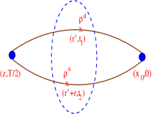
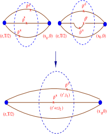
Meson	Baryon

Figure 1: Two- and three- current correlators for a meson (left) and a baryon (upper right); Lower right: two-current correlator for a baryon after integration over one relative distance. These diagrams are drawn assuming anti-periodic boundary conditions in the time direction.

All the results on the current-current correlators have been obtained on lattices of size $16^{3}\times 32$. We analyse, for the quenched case, 220 NERSC configurations at $\beta=6.0$ and, for the unquenched, 150 SESAM configurations [7] for $\kappa=0.156$ and 200 for $\kappa=0.157$ simulated at $\beta=5.6$ with two dynamical quark flavours. The physical volume of the quenched and unquenched lattices is approximately the same.

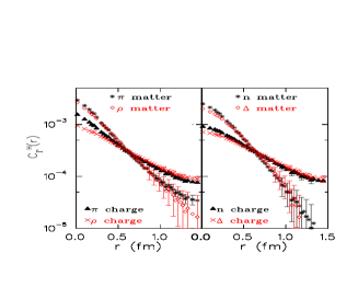
Figure 2: Quenched charge and matter distributions, $C_{\gamma_{0}}(r)$ and $C_{I}(r)$, at $\kappa=0.153$. Left for the pion and the rho; Right for the nucleon and the $\Delta$.

In Eq. 1 the current couples to the quark at fixed time separation $t$ from the source, which must be large enough to sufficiently isolate the hadron ground state. We checked, by comparing data at different $t$, that excited states are sufficiently suppressed at maximal time separation $t=T/4$ in the current-current correlators [8] where we have taken anti-periodic boundary conditions in the temporal direction. This allows us to analyse standard full QCD configurations that employ anti - periodic boundary conditions. Since, for our parameters, local sources produce the same results for $C_{\Gamma}(r)$ as smeared ones and carry no gauge noise, we use them in this study.

The quenched charge and matter density distributions were studied as a function of the naive quark mass, $m_{q}=1/2(1/\kappa-1/\kappa_{c})$, where $\kappa_{c}$ is the hopping parameter value at which the pion becomes massless. The dependence of both distributions on $m_{q}$ is more pronounced for the mesons than for the baryons. In particular the pion charge and matter distributions broaden as the quarks become lighter [9, 8]. In the case of the rho the charge distribution shows a stronger dependence on the quark mass than the matter distribution, for which no further mass dependence is observed for $m_{q}\stackrel{{\scriptstyle<}}{{\sim}}200$ MeV. For the nucleon and the $\Delta^{+}$ essentially no variation is seen over the range of naive quark masses $\sim 300-100$ MeV investigated here. The quenched charge and matter distributions are compared in Fig. 2 at $\kappa=0.153$. The matter distribution is for all hadrons less broad than the charge distribution. The root mean square radius (rms) can be extracted by evaluating

$$\hskip 56.9055pt\langle r^{2}\rangle=\frac{\sum_{\bf r}{\bf r}^{2}C_{\Gamma}({\bf r},t)}{\sum_{\bf r}C_{\Gamma}({\bf r},t)}\quad.$$ (2)

For non-relativistic states the charge rms radius can be written in terms of the form factors as [10]

$$\langle r^{2}\rangle = -\sum_{n}\nabla^{2}_{{\bf q}^{2}}F_{hn}^{u}({\bf q})F_{nh}^{d}(-{\bf q})\left.\right|_{{\bf q}^{2}=0}$$ (3)

$$= r_{u}^{2}+r_{d}^{2}-2\sum_{n}{\bf d}_{hn}^{u}.{\bf d}_{nh}^{d}\vspace*{-0.5cm}$$

where the non-relativistic form factors $F_{hn}^{u,d}({\bf q})=\langle h,{\bf q}|j_{\gamma_{0}}^{u,d}|n,{\bf 0}\rangle$ are given by

$$F_{hn}^{u,d}({\bf q})=\left\{\begin{array}[]{cc}1-r^{2}_{u,d}\>{\bf q}^{2}/6\>+{\cal O}({\bf q}^{4})&n=h\\ {\bf q}.{\bf d}_{hn}^{u,d}+{\cal O}({\bf q}^{2})&n\neq h\end{array}\right.$$ (4)

for u- and d- quarks. The dipole-dipole term appearing in Eq. 3 can be evaluated if, for instance, we assume a non-relativistic two-body system with equal masses for the u and d quarks in the center of mass frame, since then ${\bf r}_{u}=-{\bf r}_{d}$ and $<r^{2}>=2(r_{u}^{2}+r_{d}^{2})$. Only if we allow current insertions at unequal times $t_{1}$ and $t_{2}$ and take $t_{2}-t_{1}$ large enough so that intermediate excited states are sufficiently suppressed then the charge radius, for instance of the pion, is obtained from

$$\left.\frac{\partial C_{\gamma_{0}}({\bf q})}{\partial{\bf q}^{2}}\right|_{{\bf q}^{2}=0}=\left.2\frac{\partial F_{\pi}({\bf q})}{\partial{\bf q}^{2}}\right|_{{\bf q}^{2}=0}=-\frac{2}{6}\langle r^{2}_{\rm ch}\rangle\quad.$$ (5)

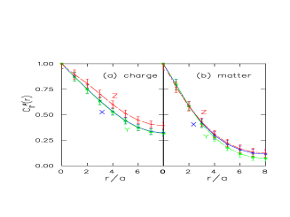
Figure 3: $C_{\Gamma}(0,0,z)$ (Z-curve); $C_{\Gamma}(x,0,0)$ and $C_{\Gamma}(0,y,0)$ ($X,Y$-curves).

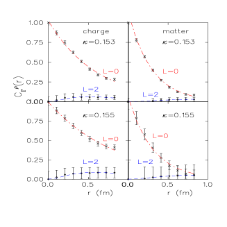
Figure 4: Decomposition into $L=0$ and $L=2$ contributions at $\kappa=0.153$ and $\kappa=0.155$. Left: charge distribution, right: matter distribution.

The rho charge density distribution [9, 11] produces a non-zero quadrupole moment or equivalently a $z-x$ asymmetry as shown in Fig. 3, where the $z$-axis is taken along the spin of the rho. This yields a deformation $\delta\equiv\frac{3}{4}\>\frac{\langle 3z^{2}-r^{2}\rangle}{\langle r^{2}\rangle}\sim 0.03\pm 0.01$ in the chiral limit. An angular decomposition of the wave function, as shown in Fig. 4, corroborates a non-zero charge deformation by producing a non-zero $L=2$ component [12]. No such deformation is seen for the matter density distribution in Figs. 3 and 4 . Since the matter and charge operators have the same non-relativistic limit, this suggests that hadron charge deformation is a relativistic effect. This result has strong implications for the validity of various phenomenological models used in the study of nucleon deformation.

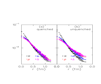
Figure 5: Quenched and unquenched charge density distributions at $\kappa=0.153$ and $\kappa=0.156$ respectively. Errors bars are omitted for clarity.

Figure 6: Quenched and unquenched matter density distributions at $\kappa=0.153$ and $\kappa=0.156$ respectively. Errors bars are omitted for clarity.

Unquenched results obtained at $\kappa=0.156$ $(m_{\pi}/m_{\rho}=0.83)$ and $\kappa=0.157$ $(m_{\pi}/m_{\rho}=0.76)$ can be compared to quenched ones at $\kappa=0.153$ $(m_{\pi}/m_{\rho}=0.84)$ and $\kappa=0.154$ $(m_{\pi}/m_{\rho}=0.78)$ having similar pion to rho mass ratios. In Figs. 5 and 6 unquenched results for $C_{\gamma_{0}}(r)$ and $C_{I}(r)$ at $\kappa=0.156$ are compared to quenched results at $\kappa=0.153$. The unquenched charge and matter distributions show an increase at short distances in the case of the pion and the rho whereas for the baryons no significant changes are seen. Like in the quenched case the unquenched matter distribution shows a faster fall-off as compared to that observed for the charge distribution. Whereas unquenching leads to an increase in the rho charge asymmetry and to a small deformation for the $\Delta^{+}$, as shown by the 3-dimensional contour plots of Fig. 7, it has no effect on the matter density distribution. This again suggests a relativistic origin for the rho charge deformation. Pion cloud contributions to hadron deformation are expected to become significant as we approach the physical pion mass and a lattice calculation with lighter pions can test if the charge rho asymmetry shows a significant increase, as suggested in some models, and at the same time if a matter density asymmetry shows up.

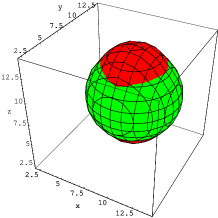
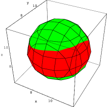
Figure 7: Three-dimensional contour plot of the charge correlator (red): upper for the rho state (cigar shape) and lower for the $\Delta^{+}$ (slightly oblate) for two dynamical quarks at $\kappa=0.156$. Values of the correlator (0.5 for the rho, 0.8 for the $\Delta^{+}$) were chosen to show large distances but avoid finite-size effects. We have included for comparison the contour of a sphere (green).

3 $\gamma N\rightarrow\Delta$ transition form factors

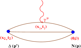
Figure 8: $\gamma N\rightarrow\Delta$ matrix element. The photon couples to a quark in the nucleon at time separation $t_{1}$ from the source to produce a $\Delta$.

We evaluate the 3-point function, $\langle G^{\Delta j^{\mu}N}_{\sigma}(t_{2},t_{1};{\bf p}^{\;\prime},{\bf p};\Gamma)\rangle$ shown schematically in Fig. 8, as well as $\langle G^{Nj^{\mu}\Delta}_{\sigma}(t_{2},t_{1};{\bf p}^{\;\prime},{\bf p};\Gamma)\rangle$ for the reverse $\Delta\rightarrow\gamma N$ transition. Exponential decays and normalization constants cancel in the ratio $R_{\sigma}(t_{2},t_{1};{\bf p}^{\;\prime},{\bf p}\;;\Gamma;\mu)=$

$$\large{\left[\frac{\langle G^{\Delta j^{\mu}N}_{\sigma}(t_{2},t_{1};{\bf p}^{\;\prime},{\bf p};\Gamma)\rangle\;\langle G^{Nj^{\mu}\Delta}_{\sigma}(t_{2},t_{1};-{\bf p},-{\bf p}^{\;\prime};\Gamma^{\dagger})\rangle}{\langle\delta_{ij}G^{\Delta\Delta}_{ij}(t_{2},{\bf p}^{\;\prime};\Gamma_{4})\rangle\;\langle G^{NN}(t_{2},-{\bf p};\Gamma_{4})\rangle}\right]^{1/2}}$$

$$\stackrel{{\scriptstyle t_{2}-t_{1}\gg 1,t_{1}\gg 1}}{{\Rightarrow}}\Pi_{\sigma}({\bf p}^{\;\prime},{\bf p}\;;\Gamma;\mu)\;,\hskip 56.9055pt(6)$$

where $G^{NN}$ and $G^{\Delta\Delta}_{ij}$ are the nucleon and $\Delta$ two-point functions evaluated in the standard way.

The Sachs form factors are obtained by appropriate combinations of the $\Delta$ spin-index $\sigma$, current direction $\mu$ and projection matrices $\Gamma$. For instance, in the $\Delta$ rest frame $\vec{p}^{\;\prime}=0\;,\;\vec{q}=(q,0,0)$  [13, 14] we have

$${\cal G}_{M1}={\cal A}\;\frac{1}{|{\bf q}|}\;\Pi_{2}({\bf 0},{\bf-q}\;;+i\;\Gamma_{4};3)$$

$${\cal G}_{E2}={\cal A}\;\frac{1}{3|{\bf q}|}\;\Biggl{[}\Pi_{3}({\bf 0},{\bf-q}\;;\Gamma_{1};3)+\Pi_{1}({\bf 0},{\bf-q}\;;\Gamma_{3};3)\Biggl{]}$$

$${\cal G}_{C2}={\cal A}\;\frac{M_{\Delta}}{{\bf q}^{\;2}}\;\Pi_{1}({\bf 0},{\bf-q}\;;-i\;\Gamma_{1};4)$$ (7)

where ${\cal A}$ is a kinematical factor.

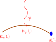
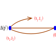
(a)	(b)

Figure 9: (a) Fixed operator and (b) fixed source sequential propagators.

We use two methods to compute the sequential propagator needed to build the 3-point function: (a) We evaluate the quark line with the photon insertion, shown schematically in Fig. 9(a) by computing the sequential propagator at fixed momentum transfer ${\bf q}$ and fixed time $t_{1}$. We look for a plateau by varying the sink-source separation time $t_{2}$. The final and initial states can be chosen at the end. (b) We evaluate the backward sequential propagator shown schematically in Fig. 9(b) by fixing the initial and final states. $t_{2}$ is fixed and a plateau is searched for by varying $t_{1}$. Since the momentum transfer is specified only at the end, the $\gamma N\rightarrow\Delta$ form factors can be evaluated at all lattice momenta.

Table 1:

$Q^{2}$ (GeV2)	$\kappa$	$m_{\pi}/m_{\rho}$	Number of confs
Quenched $\beta=6.0$ $16^{3}\times 32$ ${\bf q}^{2}=0.64$ GeV2
0.64	0.1530	0.84	100
0.64	0.1540	0.78	100
0.64	0.1550	0.70	100
Quenched $\beta=6.0$ $32^{3}\times 64$ ${\bf q}^{2}=0.64$ GeV2
0.64	0.1550	0.69	100
Quenched $\beta=6.0$ $32^{3}\times 64$ ${\bf q}^{2}=0.16$ GeV2
0.16	0.1554	0.64	100
0.15	0.1558	0.59	100
0.13	0.1562	0.50	100
Unquenched $\beta=5.6$ $16^{3}\times 32$ [7] ${\bf q}^{2}=0.54$ GeV2
0.54	0.1560	0.83	196
0.54	0.1565	0.81	200
0.54	0.1570	0.76	201
0.54	0.1575	0.68	200

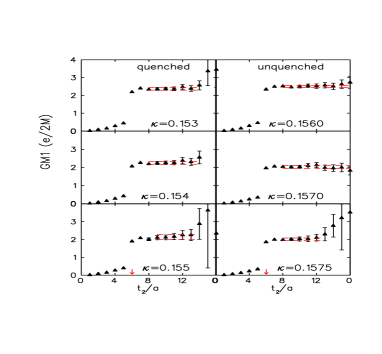
Figure 10: ${\cal G}_{M1}$ at ${\bf q}=(2\pi/16a,0,0)$ for the quenched (left) and for the unquenched (right) theory. The photon couples to the quark at $t_{1}/a=6$ as shown by the arrow. The lines show the plateau fit range and bounds obtained by jackknife analysis.

The parameters of our lattices are given in Table 1, where we used the nucleon mass in the chiral limit to convert to physical units, and $Q^{2}=-q^{2}$ is evaluated in the rest frame of the $\Delta$.

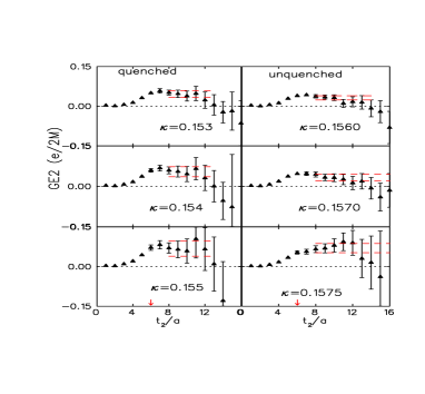
Figure 11: ${\cal G}_{E2}$ at ${\bf q}=(2\pi/16a,0,0)$. The notation is the same as that of Fig. 10.

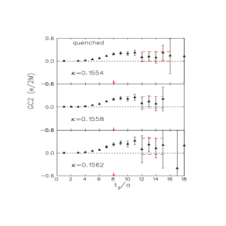
Figure 12: ${\cal G}_{C2}$ at ${\bf q}=(2\pi/32a,0,0)$ for the quenched theory. The photon couples to the quark at $t_{1}/a=8$ as shown by the arrow. The rest of the notation is the same as that of Fig. 10.

We check for finite volume effects by comparing results in the quenched theory on lattices of size $16^{3}\times 32$ and $32^{3}\times 64$ at the same momentum transfer at $\kappa=0.1550$. Assuming a 1/volume dependence we find that on the small volumes there is a $(10-15)\%$ correction as compared to the infinite volume result, whereas on the large lattice the volume correction is negligible. In Figs. 10 and 11 we show quenched and unquenched results for ${\cal G}_{M1}$ and ${\cal G}_{E2}$ at the same momentum transfer. Unquenching tends to decrease ${\cal G}_{M1}$ and ${\cal G}_{E2}$ but leaves the ratio $R_{EM}=-{\cal G}_{E2}/{\cal G}_{M1}$ largely unaffected for the SESAM quark masses studied in this work, giving values in the range of $-(2-4)\%$. The fact that no increase of $R_{EM}$ is observed means that pion contributions to this ratio are small for the SESAM pion masses. In Fig. 12 we also show results for ${\cal G}_{C2}$ with $\Delta$ static for the large quenched lattice for which we obtain the best signal. Although ${\cal G}_{C2}$ is within one standard deviation of zero, it is positive at all $\kappa$-values giving a negative ratio $R_{SM}=-|{\bf q}|/2m_{\Delta}\>{\cal G}_{C2}/{\cal G}_{M1}$ in agreement with experiment.

Chiral extrapolation of the results is done linearly in the pion mass squared, since with the nucleon or the $\Delta$ carrying a finite momentum, chiral logs are expected to be suppressed. The values obtained are given in Table 2 and are in reasonable agreement with the experimental values $R_{EM}=-2.1\pm 0.2\pm 2.0$ at $Q^{2}=0.126$ GeV² and $R_{EM}=-1.6\pm 0.4\pm 0.4$ at $Q^{2}=0.52$ GeV².

Using the fixed sink method for the sequential propagator we obtain the $q^{2}$-dependence of the form factors. In Fig. 13 we show preliminary results for

$${\cal G}_{M1}^{\star}\equiv\frac{1}{3}\frac{1}{\sqrt{1+\frac{Q^{2}}{(m_{N}+m_{\Delta})^{2}}}}\>{\cal G}_{M1}$$ (8)

obtained using 50 quenched configurations at $\kappa=0.1554$ and 0.1558, and 25 at $\kappa=0.1562$. Here we have used the ratio

$$R_{\sigma}=\frac{\langle G^{\Delta j^{\mu}N}_{\sigma}(t_{2},t_{1};{\bf p}^{\prime},{\bf p};\Gamma)\rangle}{\langle\delta_{ij}G_{ij}^{\Delta\Delta}(t_{2};{\bf p}^{\prime};\Gamma_{4})\rangle\biggl{[}\frac{\langle G^{NN}(2t_{1};{\bf p};\Gamma_{4}\rangle)}{\langle\delta_{ij}G_{ij}^{\Delta\Delta}(2t_{1};{\bf p}^{\prime};\Gamma_{4})\rangle}\biggr{]}^{1/2}}$$ (9)

to extract the form factors, since using the symmetric combination given in Eq. 3 would require an additional sequential inversion. At the lowest momentum transfer we confirm that the results from Eqs. 3 and 9 are within error bars, as shown by the data at $Q^{2}=0.13$ GeV² included in Fig. 13. The quark mass dependence is weak especially at the higher momenta and a global fit to the lattice data may be performed. The fit shows that the lattice data are consistent with a simple exponential dependence on $Q^{2}$. This fit produces a value at $Q^{2}=0$ in agreement with the Particle Data Group result [15].

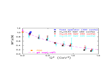
Figure 13: ${\cal G}_{M1}^{\star}$ versus $Q^{2}$ in the $\Delta$ rest frame at $\kappa=0.1554$, 0.1558 and 0.1562. The dashed line is an exponential fit to all the lattice data. The filled square is the value of ${\cal G}_{M1}^{\star}$ at $Q^{2}=0.0$ given by the Particle Data Group.

Table 2:

$Q^{2}$ GeV2	${\cal G}_{M1}\>(e/2m_{N})$	${\cal G}_{E2}\>(e/2m_{N})$	$R_{EM}\%$
Quenched QCD
0.64	1.72(6)	0.099(19)	-5.1(1.1)
0.13	2.51(6)	0.104(12)	-4.5(1.4)
Unquenched QCD
0.53	1.30(4)	0.050(31)	-2.8(1.6)

4 Conclusions

Lattice techniques are shown to be suitable for the evaluation of hadron charge and matter density distributions. Differences between quenched and unquenched results are shown to be insignificant, for both the charge and matter density distributions. The charge density distribution is, in all cases, broader than the matter density. For baryons, the lattice indicates a charge radius, which is $\sim$ 20% larger than the matter radius. The deformation seen in the rho charge distribution is absent in the matter distribution, both in the quenched and the unquenched theory. This observation suggests a relativistic origin for the deformation and deserves a more extended study, with lighter quarks and larger volumes. Nucleon deformation is signaled by a non-zero quadrupole strength in the transition $\gamma N\rightarrow\Delta$. We have calculated, for the first time using lattice QCD, the electric quadrupole form factor to high enough accuracy to exclude a zero value. The ratio $R_{EM}$ is evaluated in the kinematical regime explored by experiments. The values extracted in the chiral limit are in good agreement with recent measurements. Although large statistical and systematic errors prevent an accurate determination of the Coulomb quadrupole form factor and a zero value cannot be excluded, our results support a negative value of the ratio $R_{SM}$ in agreement with experiment. We have shown preliminary results on the $Q^{2}$ dependence of the magnetic dipole transition form factor evaluated with $\sim$ 10% accuracy in the regime explored by Jefferson Lab. The main conclusion from the analysis of the SESAM lattices [7] is that, for pions in the range of 800-500 MeV, no unquenching effects can be established for $R_{EM}$ within our statistics. We plan to repeat this calculation for lighter pions to investigate the pion cloud contributions on the transition form factors.

Acknowledgments: I am grateful to my collaborators Ph. de Forcrand, Th. Lippert, H. Neff, J. W. Negele, K. Schilling, W. Schroers and A. Tsapalis for their valuable contribution on various aspects of this work.

References

- [1]
- [2] N. Isgur, G. Karl and R. Koniuk, Phys. Rev. D 25 (1982) 2394.
- [3] G. Kälbermann and J. Eisenberg, Phys. Rev. D 28 (1982) 71; K. Bermuth, D. Drechsel, L. Tiator and J. B. Seaborn, Phys. Rev. D 38 (1988) 89.
- [4] A. J. Buchmann and E. M. Henley, Phys. Rev. C 63 (2001) 015202.
- [5] C. Mertz et al., Phys. Rev. Lett. 86 (2001) 2963; K. Joo et al., Phys. Rev. Lett. 88 (2002) 122001.
- [6] H. F. Jones and M. D. Scadron, Ann. Phys. 81, 1 (1973).
- [7] N. Eicker et al., Phys. Rev. D 59 (1999) 014509.
- [8] C. Alexandrou, Ph. de Forcrand and A. Tsapalis, Phys. Rev. D 68 (2003) 074504; hep-lat/0309064.
- [9] C. Alexandrou, Ph. de Forcrand and A. Tsapalis, Phys. Rev. D 66 (2002) 094503.
- [10] M. Burkardt, J. M. Grandy and J. W. Negele, Ann. Phys. 238 (1995) 441.
- [11] C. Alexandrou, Ph. de Forcrand and A. Tsapalis, Nucl. Phys. A721 (2003) 907; Nucl. Phys. B (Proc. Suppl.) 119 (2003) 422.
- [12] R. Gupta, D. Daniel and J. Grandy, Phys. Rev. D 48 (1993) 3330.
- [13] D. B. Leinweber, T. Draper and R. M. Woloshyn, Phys. Rev. D 48 (1993) 2230.
- [14] C. Alexandrou et al., Nucl. Phys. B (Proc. Suppl.) 119 (2003) 213; hep-lat/0307018; hep-lat/0309041.
- [15] D. E. Groom et al., European Phys. J. C15 (2000) 1.