Modelling nucleon-nucleon scattering above 1 GeV

Abstract

Motivated by the recent measurement of proton-proton spin-correlation parameters up to 2.5 GeV laboratory energy, we investigate models for nucleon-nucleon ($NN$) scattering above 1 GeV. Signatures for a gradual failure of the traditional meson model with increasing energy can be clearly identified. Since spin effects are large up to tens of GeV, perturbative QCD cannot be invoked to fix the problems. We discuss various theoretical scenarios and come to the conclusion that we do not have a clear phenomenological understanding of the spin-dependence of the $NN$ interaction above 1 GeV.

I Introduction

The force between two nucleons has been studied for many decades. Based upon the Yukawa idea [2], meson theories were developed in the 1950s [3, 4, 5, 6] and 60s [7, 8]. However when, in the 1970s, quantum chromodynamics (QCD) emerged as the generally accepted theory of strong interactions, those “meson theories” were demoted to models and the attempts to derive the nuclear force in fundamental terms had to start all over again.

The problem with a derivation from QCD is that this theory is nonperturbative in the low-energy regime characteristic for nuclear physics and direct solutions are impossible. Therefore, QCD inspired quark models were fashionable for a while—in the 1980s [10]. However, since they are—admittedly—just another set of models, they do not represent any progress in fundamental terms. If one has to resort to models anyhow, then one can, as well, continue to use meson models: they are relatively easy to build, the predictions are quite quantitative, and the underlying picture is very intuitive: mesons of increasing masses are exchanged, creating contributions of decreasing ranges until the range is sufficiently short such that it may be considered irrelevant for nuclear physics purposes.

A certain breakthrough occured, when the effective fieldtheory (EFT) concept was introduced and applied to low-energy QCD [11]. Based upon these ideas, Weinberg showed in 1990 [12], that a systematic expansion of the nucleon-nucleon ($NN$) amplitude exists in terms of $(Q/\Lambda_{\chi})^{\nu}$, where $Q$ denotes a generic nucleon momentum, $\Lambda_{\chi}\approx 1$ GeV is the chiral symmetry breaking scale, and $\nu\geq 0$. This is known as chiral perturbation theory ($\chi$PT) which is equivalent to low-energy QCD.

Weinberg’s initial work [12] created a lot of interest and activity [13, 14, 15] that has been going on now for more than a decade [16, 17, 18, 19]. As a result, we have today a rather precise understanding of the nuclear force in terms of $\chi$PT [20, 21, 22]. However, the energy range appropriate for $\chi$PT is very limited; afterall, $\chi$PT is a low-momentum expansion, good only for momenta $Q\ll\Lambda_{\chi}\approx 1$ GeV. The most advanced calculations to date go to fourth order [21, 22] at which $NN$ scattering can be described satisfactorily up to lab. energies ($T_{\rm lab}$) of about 300 MeV. For higher energies, more orders must be included. However, since the number of terms increases dramatically with each higher order (cf. Ref. [21]), $\chi$PT will be unpractical and unmanagable around order five or six. It is, thus, safe to state that $\chi$PT is limited to $T_{\rm lab}<0.5$ GeV.

There is, of course, a need to understand $NN$ scattering also above 0.5 GeV. Naively one might expect that perturbative QCD (pQCD) should be useable above the scale of the low-energy EFT. Unfortunately, this is not true. Energies of the order of 1 GeV are far too low to invoke pQCD. Thus, in the energy range that stretches from about 0.5 GeV to, probably, tens of GeV, we are faced with the dilemma that we have presently no calculable theory at our disposal. In principal, it should be possible to apply lattice QCD in this energy regime. However, such calculations are not available, at this time. They are an interesting prospect for the future.

For theoretical physics, it is not uncommon to encounter such problems. Typically, the preliminary way out is to build models. The hope is that reasonably constructed models may provide insight which may ultimately lead to a solution on more fundamental grounds. The ‘standard model’ for the nuclear force is relativistic meson-exchange. In the past, meson models have been constructed and shown to describe $NN$ scattering up to about 1 GeV satisfactorily [9, 23, 24, 25, 26, 27, 28, 29, 30, 31, 32].

However, above 1 GeV, there remains a large energy range where pQCD is still not applicable. Traditionally, this energy region has been the stepchild of the theoretical profession. Recently, a large number of precise $pp$ scattering data up to 2.8 GeV have been measured [33, 34, 35, 36, 37, 38]. The obvious question is: Do we understand these data, their angular and energy dependence? The focus of this paper will be on the spin observables that are more exclusive than the spin averaged cross sections.

This paper is organized as follows. In Sec. II, we present a typical model that is known to be appropriate for energies up to about 1 GeV. In Sec. III, this model is applied for energies above 1 GeV, and some modifications necessary for those higher energies are introduced. Sec. IV is then devoted to spin observables. We conclude the paper with Sec. V, where we elaborate on the unsolved problems of the energy region under consideration.

II Relativistic meson-exchange model for $NN$ scattering at intermediate energies

The simplest meson model for the nuclear force is the so-called one-boson-exchange (OBE) model which takes only single-particle exchanges into account [39]. Typically, the mesons with masses below the nucleon mass are included. Most important, are the following four mesons:

• The pseudoscalar pion with a mass of about 138 MeV. It is the lightest meson and provides the long-range part of the potential and most of the tensor force.

• The $\rho$ meson, a 2$\pi$ $P$-wave resonance of about 770 MeV. Its major effect is to cut down the tensor force provided by the pion at short range—to a realistic size.

• The $\omega$ meson, a 3$\pi$ resonance of 783 MeV and spin 1. It creates a strong repulsive central force of short range (‘repulsive core’) and most of the nuclear spin-orbit force.

• The $\sigma$ boson of about 550 MeV. It provides the intermediate range attraction necessary for nuclear binding and can be understood as a simulation of the correlated $S$-wave 2$\pi$-exchange.

Besides these four bosons, we include also the $\eta(547)$, which brings the total number to five. The quantum numbers characterizing these mesons (like, spin, parity, isospin) are shown in Table I.

The following Lagrangians describe the coupling of these mesons to nucleons:

$${\cal L}_{pv} = -\frac{f_{ps}}{m_{ps}}\bar{\psi}\gamma^{5}\gamma^{\mu}\psi\partial_{\mu}\varphi^{(ps)}$$ (1)

$${\cal L}_{s} = -g_{s}\bar{\psi}\psi\varphi^{(s)}$$ (2)

$${\cal L}_{v} = -g_{v}\bar{\psi}\gamma^{\mu}\psi\varphi^{(v)}_{\mu}-\frac{f_{v}}{4M}\bar{\psi}\sigma^{\mu\nu}\psi(\partial_{\mu}\varphi_{\nu}^{(v)}-\partial_{\nu}\varphi_{\mu}^{(v)})$$ (3)

where $M$ is the nucleon mass and $m_{\alpha}$ a meson mass. $\psi$ denotes the nucleon and $\varphi^{(\alpha)}_{(\mu)}$ the meson fields (notation and conventions as in Ref. [40]). For isospin-1 (isovector) mesons, $\varphi^{(\alpha)}$ is to be replaced by $\tau\cdot\varphi^{(\alpha)}$ with $\tau^{i}$ ($i=1,2,3$) the usual Pauli matrices. $ps$, $pv$, $s$, and $v$ denote pseudoscalar, pseudovector, scalar, and vector couplings/fields, respectively. For the pseudoscalar mesons $\pi$ and $\eta$, we use the pseudovector coupling, Eq. (1), as suggested by chiral symmetry. The scalar boson $\sigma$ couples via the scalar Lagrangian, Eq. (2), and the vector mesons $\rho$ and $\omega$ interact through the Lagrangian Eq. (3). The coupling constants, $g_{\alpha}$ and $f_{\alpha}$, are given in Table I in terms of $g^{2}_{\alpha}/4\pi$ and $f^{2}_{\alpha}/4\pi$, respectively.

Based upon the above Langrangians, the one-particle-exchange Feynman diagrams (Fig. 1) can be evaluated straightforwardly (see Ref. [9] for details). The OBE potential is then defined as the sum of the Feynman amplitudes created from the five mesons:

$$\bar{V}=\sum_{\alpha=\pi,\eta,\sigma,\rho,\omega}\bar{V}_{\alpha}$$ (4)

Explicit expressions for the Feynman amplitudes, $\bar{V}_{\alpha}$, can be found in Refs. [9, 41]. We note that we modify these Feynman amplitudes by applying, at each meson-nucleon vertex, a form factor which has the analytical form

$$F_{\alpha}[(\vec{q^{\prime}}-{\vec{q}})^{2}]=\left(\frac{\Lambda^{2}_{\alpha}-m^{2}_{\alpha}}{\Lambda^{2}_{\alpha}+(\vec{q^{\prime}}-{\vec{q}})^{2}}\right)^{n_{\alpha}}\,,$$ (5)

where $\vec{q}$ and $\vec{q^{\prime}}$ denote the nucleon momenta in the center-of-mass (c.m.) frame in the initial and final state, respectively; and $(\vec{q^{\prime}}-\vec{q})$ is the momentum transfer between the two interacting nucleons. $\Lambda_{\alpha}$ is called the cutoff mass. We use $n_{\alpha}=1$ for all vertices with the exception of the $N\Delta\rho$ vertex where $n_{\alpha}=2$ is applied (s. below). The form factor suppresses the contributions from high momentum transfer which is equivalent to short distances. This is necessary to make loop integrals (and the solution of the Lippmann-Schwinger equation) convergent and suggested by the extended (quark) substructure of hadrons.

For the energies to be considered in this study, it is mandatory to use a relativistic formalism. Relativistic $NN$ scattering is described by the Bethe-Salpeter equation [42]. Unfortunately, this four-dimensional equation is difficult to solve. Therefore, so-called three-dimensional reductions have been proposed which are more amenable to numerical solution. We will use the relativistic three-dimensional Thompson equation [43] which reads,

$$\bar{T}(\vec{q^{\prime}},\vec{q};\sqrt{s})=\bar{V}(\vec{q^{\prime}},\vec{q})+\int d^{3}k\>\bar{V}(\vec{q^{\prime}},\vec{k})\>\frac{M^{2}}{E_{k}^{2}}\>\frac{1}{\sqrt{s}-2E_{k}+i\epsilon}\>\bar{T}(\vec{k},\vec{q};\sqrt{s})\,,$$ (6)

where $\bar{T}$ denotes the invariant scattering amplitude and $\sqrt{s}$ is the total energy in the c.m. frame; $\sqrt{s}=2E_{q}$ with $E_{q}\equiv\sqrt{q^{2}+M^{2}}$ and $q\equiv|\vec{q}|$ the momentum of one nucleon in the c.m. frame, which is related to the lab. energy of the projectile by $T_{\rm lab}=2q^{2}/M$. It is convenient to define

$${T}(\vec{q^{\prime}},\vec{q})={\frac{M}{E_{q^{\prime}}}}\>\bar{T}(\vec{q^{\prime}},\vec{q})\>{\frac{M}{E_{q}}}$$ (7)

and

$${V}(\vec{q^{\prime}},\vec{q})={\frac{M}{E_{q^{\prime}}}}\>\bar{V}(\vec{q^{\prime}},\vec{q})\>{\frac{M}{E_{q}}}\>.$$ (8)

With this, we can rewrite Eq. (6) as

$${T}(\vec{q^{\prime}},\vec{q};\sqrt{s})={V}(\vec{q^{\prime}},\vec{q})+\int d^{3}k\>{V}(\vec{q^{\prime}},\vec{k})\frac{1}{\sqrt{s}-2E_{k}+i\epsilon}{T}(\vec{k},\vec{q};\sqrt{s})$$ (9)

which resembles a Lippmann-Schwinger equation with relativistic energies.

In the framework of the relativistic three-dimensional reduction of the Bethe-Salpeter equation applied here (Thompson equation), the OBE potential is real at all energies and, therefore, suitable only for $NN$ scattering below the inelastic threshold. Above $T_{\rm lab}\approx 290$ MeV, pions can be produced in $NN$ collisions. A model that is expected to have validity at intermediate energies needs to take the inelasticity due to pion-production into account. It is well-known that, below about 1.5 GeV, pion production proceeds mainly through the formation of the $\Delta(1232)$ isobar which is a pion-nucleon resonance with spin and isospin 3/2. The next higher resonance is the $N^{*}(1440)$, also known as Roper resonance, with spin and isospin 1/2 [44]. This resonance was included in a meson model for $NN$ scattering up to 2 GeV constructed by Lee [45] and found to contribute less than 1 mb to the inelastic cross section even at 2 GeV. A recent exclusive measurement of two-pion production in $pp$ scattering at 775 MeV finds cross sections that can be attributed to the Roper resonance of less than 0.1 mb [46]. Thus below 2 GeV, the $N^{*}(1440)$ is much less important than the $\Delta(1232)$. Therefore, we introduce only the $\Delta$ as an additional degree of freedom. Consequently, we have now, besides the $NN$ channel, two more two-baryon channels, namely, $N\Delta$ and $\Delta\Delta$.

Since all channels have baryon number two, transitions between these channels are allowed, i. e., the channels “couple”. Mathematically this produces a system of coupled equations for the scattering amplitudes. In operator notation, one can write:

$$T_{ij}=V_{ij}+\sum_{k}V_{ik}\>g_{k}\>T_{kj}\,,$$ (10)

where each subscript $i,j,$ and $k$ denotes a two-baryon channel ( $NN$, $N\Delta$, or $\Delta\Delta$), and $g_{k}$ is the appropriate two-baryon propagator. In principal, there are nine transition potentials, $V_{ij}$, which reduce to six due to time-reversal. Three of them, namely, $V_{N\Delta,N\Delta}$, $V_{N\Delta,\Delta\Delta}$, $V_{\Delta\Delta,\Delta\Delta}$, involve $\Delta\Delta\alpha$ vertices, where $\alpha$ is a non-strange meson. Exploiting the usual symmetries, such vertices can be constructed; however, there is no way to test empirically if the assumptions about these vertices are realistic. Therefore, such constructs are beset with large uncertainties, which is why we omit them. The consequence is that the system of coupled equations, Eq. (10), decouples and the $T$-matrix of $NN$ scattering, $T\equiv T_{NN,NN}$, is the solution of just one integral equation:

$$T=V_{\rm eff}+V_{\rm eff}\;g_{NN}\;T\,,$$ (11)

with

$$V_{\rm eff}=V_{NN,NN}+V_{NN,N\Delta}\;g_{N\Delta}\;V_{N\Delta,NN}+V_{NN,\Delta\Delta}\;g_{\Delta\Delta}\;V_{\Delta\Delta,NN}\,,$$ (12)

where $V_{NN,NN}$ is the $V$ given in Eq. (8) which is based upon Eq. (4) and shown in Fig. 1. The last two terms on the r.h.s. of the above equation are depicted in Fig. 2.

Because of isospin conservation, the transition potentials containing $N\Delta\alpha$ vertices can only involve isovector mesons. Thus,

$$V_{NN,N\Delta} = \sum_{\alpha=\pi,\rho}V^{\alpha}_{NN,N\Delta}\,,$$ (13)

$$V_{NN,\Delta\Delta} = \sum_{\alpha=\pi,\rho}V^{\alpha}_{NN,\Delta\Delta}\,.$$ (14)

The amplitudes, $V^{\alpha}_{NN,N\Delta}$ and $V^{\alpha}_{NN,\Delta\Delta}$, with $\alpha=\pi,\rho$, are derived from the interaction Langrangians:

$${\cal L}_{N\Delta\pi} = -\frac{f_{N\Delta\pi}}{m_{\pi}}\bar{\psi}{\bf T}\psi^{\mu}\partial_{\mu}{\mbox{\boldmath$\varphi$}}^{(\pi)}+{\rm H.c.}\,,$$ (15)

$${\cal L}_{N\Delta\rho} = i\frac{f_{N\Delta\rho}}{m_{\rho}}\bar{\psi}\gamma^{5}\gamma^{\mu}{\bf T}\psi^{\nu}(\partial_{\mu}{\mbox{\boldmath$\varphi$}}^{(\rho)}_{\nu}-\partial_{\nu}{\mbox{\boldmath$\varphi$}}_{\mu}^{(\rho)})+{\rm H.c.}\,,$$ (16)

where $\psi_{\mu}$ is a Rarita-Schwinger field [47, 48, 49] describing the (spin $\frac{3}{2}$) $\Delta$-isobar and ${\bf T}$ denotes an isospin transition operator that acts between isospin-$\frac{1}{2}$ and isospin-$\frac{3}{2}$ states. H.c. stands for hermitean conjugate. The transition potentials $V^{\pi}_{NN,N\Delta}$ and $V^{\pi}_{NN,\Delta\Delta}$ can be found in Ref. [50] and $V^{\rho}_{NN,N\Delta}$ and $V^{\rho}_{NN,\Delta\Delta}$ are given in Ref. [51]. We use these relativistic transition potentials in conjunction with static meson propagators that take the delta-nucleon mass difference into account. The vertices involved in the transition potentials are multiplied with form factors of the type Eq. (5).

The two-baryon propagators involved in Eqs. (11) and (12) are,

$$g_{NN} = \frac{1}{\sqrt{s}-2E_{k}+i\epsilon}\,,$$ (17)

$$g_{N\Delta} = \frac{1}{\sqrt{s}-E_{k}-\tilde{E}^{\Delta}_{k}(\sqrt{s})}\,,$$ (18)

$$g_{\Delta\Delta} = \frac{1}{\sqrt{s}-2\tilde{E}^{\Delta}_{k}(\sqrt{s})}\,,$$ (19)

where $\tilde{E}^{\Delta}_{k}(\sqrt{s})=\sqrt{k^{2}+\tilde{M}_{\Delta}^{2}(\sqrt{s})}$ with $\tilde{M}_{\Delta}(\sqrt{s})=M_{\Delta}-i\Gamma(\sqrt{s})/2$ a complex $\Delta$-mass. The real part of the $\Delta$ mass is the wellknown physical mass, $M_{\Delta}=1232$ MeV. The imaginary part, which is associated with the decay-width of the $\Delta$-isobar, creates the inelasticity in our model and simulates pion production. It is calculated from the self-energy of the $\Delta$-isobar that is obtained from a solution of the Dyson equation in which the $\Delta$ is coupled virtually to the $\pi N$ decay channel [27, 28, 30]. $\Gamma(\sqrt{s})$, is energy-dependent and the threshold is $\sqrt{s}=2M+m_{\pi}$ for diagrams with one intermediate $\Delta$ state and $\sqrt{s}=2M+2m_{\pi}$ for two intermediate $\Delta$. Below these thresholds, $\Gamma(\sqrt{s})$ vanishes. Note that, due to isospin conservation, $N\Delta$ diagrams contribute only in isospin $T=1$ $NN$-states, while $\Delta\Delta$ diagrams contribute to all states. Consequently, in $T=0$, only double-$\Delta$ diagrams contribute (besides the usual OBE contributions, Fig. 1). This explains the thresholds for inelasticity seen in Fig. 3.

The model developed so far consists of the diagrams displayed in Figs. 1 and 2 (using the complex propagators discussed above). These diagrams make up the “effective” $NN$ potential, Eq. (12), that is applied in the scattering equation, Eq. (11), to determine the $NN$ $T$-matrix, from which phase parameters and observables can be calculated. It is wellknown that models of this kind [27, 28, 30, 55] are able to describe $NN$ scattering up to about 1 GeV in semi-quantitative terms. Using the parameters listed in Table I, phase shifts and inelasticity parameters are predicted as shown in Fig. 3 and mixing parameters as in Fig. 4. It is seen that several phase shifts are predicted quantitatively, notably the $S$ waves; others are semi-quantitative, like the $P$ waves which, typically, show too much attraction at intermediate energies. The cusps that are known to be the signature of the $\Delta$ threshold [56] also show up clearly: the shape of the ${}^{1}D_{2}$ phase shift is well reproduced while, in ${}^{3}F_{3}$ and ${}^{3}P_{2}$, only the trends are right. Inelasticities are by and large described well, but in the crucial cases, namely, ${}^{1}D_{2}$ and ${}^{3}F_{3}$ the inelasticity is predicted too small. This is a wellknown problem [27, 28, 30]. However, over-all we perceive the agreement between predicted and empirical phase parameters displayed in Figs. 3 and 4 as sufficient to conclude that we have a satisfactory understanding of $NN$ scattering up to about 1 GeV in terms of a relativistic meson model extended by the $\Delta(1232)$ resonance.

III The energy regime above 1 GeV

With this section, we will start to investigate the issue to which extend the relativistic meson model of the previous section can be stretched beyond 1 GeV. We will consider, first, the most inclusive observables, namely, total cross sections. The predictions for the total elastic and the total (i. e., elastic plus inelastic) cross sections are shown in Fig. 5 for energies up to 5 GeV laboratory energy [57]. From the figure, one can make two important observations:

• The predicted inelasticity (difference between the dashed and solid curve in Fig. 5) is substantially too small above 1 GeV.

• The predicted elastic cross section rises with energy while, empirically, it drops.

The lack of inelasticity is not unexpected since, for $T_{\rm lab}>1$ GeV, the effectiveness of the $\Delta(1232)$ resonance is diminishing, while other inelastic processes enter the picture which are not included in our model. However, the number of inelastic channels that open above 1 GeV increases so rapidly with energy [44] that it would be inefficient to take them into account one by one. Except for the shoulder around $T_{\rm lab}\approx 800$ MeV which is due to the $\Delta$ resonance, the inelastic cross section is smooth and does not show any structures that would be indicative for the outstanding role of another meson-nucleon resonance or a particular inelastic channel. Hence, a picture of many overlapping resonances and inelastic channels emerges which suggests that further inelasticity can be pragmatically described by a smooth optical potential.

In configuration space ($r$-space) calculations, the following form has been used for a nonrelativistic optical potential [58]:

$$\tilde{V}_{\rm opt}(r,s)=\left[\tilde{V}_{0}(s)+i\tilde{W}_{0}(s)\right]\exp\left(-\frac{r^{2}}{a^{2}}\right)\,,$$ (20)

where, as before, $s$ denotes the square of the total c.m. energy. The Gaussian shape is suggested by the geometrical picture proposed by Chou and Yang [59], in which two colliding nucleons are described as extended objects made from some kind of hadronic matter that has a distribution similar to the charge distribution. The proton electromagnetic form factor is well represented by a Gaussian.

Since we work in momentum space, we Fourier transform Eq. (20), yielding

$$\hat{V}_{\rm opt}(k,s)=\left(\frac{\sqrt{\pi}a}{2\pi}\right)^{3}\left[\tilde{V}_{0}(s)+i\tilde{W}_{0}(s)\right]\exp\left(-\frac{k^{2}a^{2}}{4}\right)\,.$$ (21)

This is a nonrelativistic scalar. However, our approach is relativistic and, therefore, all contributions must have a proper Lorentz-Dirac structure. In analogy to the nonrelativistic approach, the obvious choice is a Lorentz scalar [60] which we define as follows (using the formalism of Refs. [9] and [41]):

$$\langle\vec{q^{\prime}}\lambda_{1}^{\prime}\lambda_{2}^{\prime}|\bar{V}_{\rm opt}|{\vec{q}}\lambda_{1}\lambda_{2}\rangle=\hat{V}_{\rm opt}(k,s)\left[\bar{u}(\vec{q^{\prime}},\lambda_{1}^{\prime})u({\vec{q}},\lambda_{1})\right]\left[\bar{u}(-\vec{q^{\prime}},\lambda_{2}^{\prime})u(-{\vec{q}},\lambda_{2})\right]\,,$$ (22)

where $\lambda_{1},\lambda_{2}$ ($\lambda_{1}^{\prime},\lambda_{2}^{\prime}$) denote the helicities of the two ingoing (outgoing) nucleons and $\vec{q}$ ($\vec{q^{\prime}}$) are the corresponding relative momenta in the c.m. system; $k\equiv|\vec{q^{\prime}}-\vec{q}|$ is the magnitude of the momentum transfer between the interacting nucleons. The Dirac spinors in helicity representation are given by

$$u({\vec{q}},\lambda_{1}) = \sqrt{\frac{E_{q}+M}{2M}}\left(\begin{array}[]{c}1\\ \frac{2\lambda_{1}|{\vec{q}}|}{E_{q}+M}\end{array}\right)|\lambda_{1}\rangle\>,$$ (25)

$$u(-{\vec{q}},\lambda_{2}) = \sqrt{\frac{E_{q}+M}{2M}}\left(\begin{array}[]{c}1\\ \frac{2\lambda_{2}|{\vec{q}}|}{E_{q}+M}\end{array}\right)|\lambda_{2}\rangle\>,$$ (28)

which are normalized such that

$$\bar{u}({\vec{q}},\lambda)u({\vec{q}},\lambda)=1\,,$$ (29)

with $\bar{u}=u^{\dagger}\gamma^{0}$.

Instead of fitting the parameters of the optical potential, $\tilde{V}_{0}(s)$ and $\tilde{W}_{0}(s)$, separately for various single energies [58, 60], we find it physically more reasonable to choose a smooth, analytic function of $s$ with the correct high-energy behavior built in:

$$\tilde{V}_{0}(s)+i\tilde{W}_{0}(s)=\left\{\begin{array}[]{ll}0&\mbox{for $T_{\rm lab}\leq T_{\rm lab}^{(0)}$}\\ \left(\frac{s-s_{0}}{4M^{2}}\right)[V_{0}+iW_{0}]&\mbox{for $T_{\rm lab}>T_{\rm lab}^{(0)}$}\,,\end{array}\right.$$ (30)

where $s_{0}=2M(2M+T_{\rm lab}^{(0)})$ and $T_{\rm lab}^{(0)}=0.8$ GeV. This parametrization implies that the optical potential is proportional to $s$ for large energies ($s\gg s_{0}$) which leads to constant total cross section predictions in the energy range 10 to 100 GeV, consistent with experiment [44].

In summary, to generate the additional inelasticity required for the total cross sections above about 1 GeV, we add to the model developed in Sec. II the relativistic optical potential defined by Eqs. (22), (21) and (30).

We now turn to the other deficiency that we are observing in Fig. 5, namely, the rise of the elastic cross section with energy, which contradicts experiment. One-particle exchange creates amplitudes that have the basic mathematical structure

$$\bar{V}_{\alpha}\propto\frac{s^{J}}{t-m_{\alpha}^{2}}$$ (31)

where $J$ denotes the spin of the exchanged particle and $t$ is the square of its four-momentum. The vector mesons $\rho$ and $\omega$ have $J=1$ and, therefore, create total cross sections that rise with $s$. This is the basic reason for the rising cross sections seen in Fig. 5.

This failure of the one-particle exchange picture at high energies has been known since the late 1950’s, when data of sufficient energy became available to reveal this problem. In an attempt to solve this problem, Regge theory [61, 62, 63] was developed in the early 1960’s which, indeed, is able to reproduce the general energy behavior of two-body cross sections, correctly. In the Regge model, one-particle exchange is replaced by the exchange of a Regge pole, which is an infinite series of particles with the same spin, isospin, and strangeness, aligned along a Regge trajectory. Regge trajectories are named by their first, best-known family member: there exists a $\rho$ and an $\omega$ trajectory.

Based upon these historical developments, it might be appealing to replace the one-rho and one-omega exchanges in our model by the corresponding Regge trajectories. However, there are reasons why we should not resort to such drastic measures. From a modern point of view, Regge theory is essentially a phenomenology for very high energies. It is most appropriate above about 10 GeV which is beyond the energies that we are intersted in. This fact reveals the greatest dilemma of the energy regime between 1 and 10 GeV: there exist well-tested models below 1 GeV (meson model) and above 10 GeV (Regge model), however in-between, the established models are partially inadequate and no alternatives have been proposed.

Another problem with Regge theory is that it does not make any predictions for the spin-dependence of the interaction, which is one focus of this study (see below).

For the reasons discussed, we will not switch to Regge theory. Instead, we will modify our model in the spirit of Regge theory. Of the Regge trajectories, we will only keep the first family member. The one-particle exchange amplitude of this first member will be modified such that the main effect of the rest of the trajectory is taken into account. As discussed, this main effect is that it removes the wrong energy behavior from the amplitude. Thus, we apply to the one-omega and one-rho exchange amplitudes a factor that divides the wrong energy dependence out:

$$\bar{V}_{\alpha}\longmapsto\frac{s_{0}}{s}\bar{V}_{\alpha}\,,$$ (32)

for $\alpha=\rho,\omega$ and $s>s_{0}$ with $s_{0}$ as defined below Eq. (30). For $s\leq s_{0}$, there are no changes. The modification, Eq. (32), is applied to the $\rho$ and $\omega$ exchanges of $V_{NN,NN}$ and the $\rho$ exchanges of $V_{NN,N\Delta}$ and $V_{NN,\Delta\Delta}$ [cf. Eq. (12)].

Including the optical potential, Eq. (22), and the modification of the vector meson amplitudes, Eq. (32), we obtain the total cross section predictions displayed in Fig. 6. The elastic cross section now shows the correct energy behavior and the inelasticity (and the total cross section) is of the right size and energy dependence. Thus, based upon a few physically reasonable assumptions, it is fairly easy and straightforward to describe the $pp$ total cross sections above 1 GeV.

IV Spin observables

In this section, we turn to $pp$ spin observables. We will compare predictions by the model developed in the previous two sections (and variations thereof) to data for five representative energies in the range 400 MeV to 2500 MeV. Besides differential cross sections, $d\sigma/d\Omega$, and analyzing powers, $A_{N}$, we will consider the spin correlation coefficients $A_{NN}$, $A_{SS}$, $A_{SL}$, and $A_{LL}$, for which (except for $A_{LL}$) precise data have been taken by the EDDA group  [33, 34, 35], and for $A_{NN}$, $A_{SL}$ at SATURNE [36, 38]. Since the differences between the two experimental data sets are small as compared to the difference between theory and experiment, we will subsequently compare only to the EDDA data.

The predictions by the relativistic meson model presented in Sec. II, as modified in Sec. III, are shown by the solid curve in Fig. 7. The dashed curve in the figure is obtained when the optical potential, Eq. (22), and the corrections to vector meson, Eq. (32), are left out. Finally, the dotted curve is based upon the GWU (formerly VPI) phase shift analysis SP03 [53]. Since a phase shift analysis is just an alternative way of representing data, the dotted curve follows, in general, the data included in Fig. 7. The exception is $A_{LL}$, where no data exist and where, therefore, the analysis represents the only empirical information to compare with.

Since we expect the meson model to be right at least for low energies, it is comforting to see that at 400 MeV there is generally good agreement between theory and experiment for all observables shown. Consistent with the predictions for total cross sections discussed in Sec. III, the differential cross sections come out too large above 1 GeV when the modifications introduced in Sec. III are not applied (dashed curve). Including those modifications (solid curve) yields a better agreement for all energies up to 2.5 GeV, for differential cross sections.

However, for spin observables, the agreement is much less satisfactory. Already at 800 MeV, the analyzing power is predicted substantially too high, which is probably associated with the fact that the ${}^{3}P_{2}$ phase shift is predicted too large above 650 MeV (cf. Fig. 3); note that only spin-triplet partial waves enter the amplitudes describing $A_{N}$.

At higher energies, the corrections necessary to improve the cross sections enhance $A_{N}$ contrary to the data. So, overall, the analyzing power is predicted persistently too large.

In the case of the spin correlation parameters, the correction applied to vector-meson exchange, Eq. (32), and the optical potential provide effects that point in the right direction. Nevertheless, the best one can say is that theory and experiment agree in the trends that the spin correlation coefficients show as a function of angle. But, in quantitative terms, there are large discrepancies.

The parameters of our model are the meson-baryon coupling constants and the cutoff masses, which parametrize the meson-baryon form factors. With the exception of the $\pi NN$ and $\pi N\Delta$ coupling constants, these parameters are only losely constrained by information from other sources. Consequently, the parameter set that we have used so far is not the only choice that can be made. Therefore, we have varied all parameters within the ranges given in Table I. These ranges represent educated estimates of the uncertainties. The result of this very comprehensive investigation of a systematic variation of all parameters can be summarized as follows: It is not possible to obtain a fit of all observables at all energies considered that is substantially better than the one shown in Fig. 7.

To obtain further insight into the nature of the problem, we have investigated the question, if it is at least possible to fit single observables at single energies. We selected a few representative cases and found for all of them that it was, indeed, possible to find a combination of parameters that resulted in a good fit of the single observable chosen. To illustrate this point, we show in Fig. 8 the case where the prediction for $A_{N}$ at 1.8 GeV is substantially improved. However, it is clearly seen that the fit of all the other observables is now, in general, worse than in Fig. 7, including $A_{N}$ at lower energies. Thus, the quantitative fit of just one observable at one energy and for a limited range of angles cannot be perceived as a confirmation of the validity of the meson model at high energies [64]. On the other hand, the fact that all observables can be fitted separately by some individually adjusted combination of parameters implies that our model does contain all the types of spin-dependent forces necessary to describe the $NN$ amplitudes. What fails is the energy- and angle-dependence. While for low energies (below $\approx 0.8$ GeV) the meson model generates the correct energy-dependence for the strength of the various spin-dependent components, this energy-dependence becomes increasingly wrong when proceeding to higher energies.

V Conclusions

In this paper, we have studied $NN$ scattering above 1 GeV laboratory energy. We started from a model that is based upon relativistic meson-exchange, complemented by the $\Delta(1232)$ isobar, and reproduces $NN$ scattering up to about 1 GeV satisfactorily. We have then extrapolated this model above 1 GeV. At those higher energies, characteristic deficiencies in the total and differential cross sections show up that are easy to fix. The lack of inelasticity is mended by introducing an optical potential of the shape of the proton form factor. The well-known wrong high-energy behavior of vector-meson exchange becomes noticable already around 1.2 GeV. In the spirit of Regge theory, we apply a factor $s_{0}/s$ to vector mesons with the consequence that the elastic cross sections and their energy behavior are predicted correctly.

An important focus of our study have been spin-observables of $pp$ scattering. Due to recent experiments conducted by the EDDA group [34, 35], data on spin correlation coefficients (besides analyzing powers) up to 2.5 GeV are now available for a broad range of angles. Comparison of our predictions with these data confirms the well-known fact that a correct reproduction of cross sections by no means implies a correct description of spin observables. Even the “simplest” spin observable, namely, the analyzing power $A_{N}$, poses a challenge to theory which predicts $A_{N}$ persistently too large. Concerning the more sophisticated spin correlation parameters, the only encouraging statement that can be made is that the characteristic trends of these observables as a function of angle come out about right. But there is no quantitative agreement. Varying the parameters of the model (coupling constants and cutoff parameters) over a wide range does not improve the over-all quality of the description of the data.

In conclusion, we do not have a quantitative understanding of the spin-dependence of the $NN$ interaction above 1 GeV. The meson model, which is so successful at low energies, becomes increasingly inadequate above 1 GeV. This fact is revealed most clearly by spin observables.

It is tempting (since plausible) to interpret the gradual failure of the meson model with increasing energy as an indication that pQCD is becoming the valid approach at higher energy. Unfortunately, this suggestion is not correct. The implications of pQCD for $NN$ elastic scattering have been worked out carefully in Ref. [65] and the prediction clearly is:

$$A_{N}=0$$ (33)

at all angles. This is not what we see in the data. In fact, $A_{N}$ was measured up to laboratory energies of 28 GeV by Alan Krisch and the Michigan group [66] and there are no indications for a decline of $A_{N}$ even at those large energies.

Assuming massless, effectively free quarks, the helicities of the quarks are conserved, which implies for the spin-correlations parameters [65]:

$$A_{NN} = -A_{SS}\,,$$ (34)

$$A_{SL} = 0\,,$$ (35)

for all angles. Applying the quark-interchange model to this scenario, yields the specific predictions [65]

$$A_{NN}(90^{0}) = \frac{1}{3}\,,$$ (36)

$$A_{LL}(90^{0}) = A_{SS}(90^{0})=-\frac{1}{3}\,,$$ (37)

which (as it should) satisfies the model-independent sum rule:

$$A_{NN}(90^{0})-A_{LL}(90^{0})-A_{SS}(90^{0})=1\,,$$ (38)

where the angle is measured in the c.m. system.

Accidentally, the data at 800 MeV and above displayed in Fig. 7 agree roughly with Eqs. (34) and (35). However, we should not interpret this as a signature of pQCD. The Michigan group [66] measured $A_{NN}$ at $90^{0}$ up to 12 GeV and found strong variations with energy, and a value of about 0.6 at 12 GeV which disagres by a factor two with Eq. (36). Moreover, the best-founded implication of pQCD is a vanishing analyzing power and, therefore, if this condition is not met, we are not in pQCD territory.

In lack of a calculable high-energy theory, one may consider to resort to traditional high-energy phenomenology. The Regge model complemented by Pomeron exchange is the most successfull phenomenology for the description of hadron-hadron cross sections above 10 GeV laboratory energy [67, 68]. However, the main problem that we are facing in this study are spin observables. To our knowledge, the exact implications of Regge theory for the spin-dependence of the $NN$ interaction has never been worked out, since most of the work on Regge theory was done in the 1960s when polarization data at high energy were not available. The work by Rijken [69] on low-energy implications of Regge theory suggests that Regge theory predicts a spin-dependence similar to the OBE model. If true, then our model contains already all the spin-dependence that a Regge theory would produce. On the other hand, one may also raise objections concerning the use of Regge theory: In general, the Regge model is perceived as appropriate in the energy regime above 10 GeV and, so, it is questionable if it is the right phenomenology for energies at a few GeV which is our focus.

In summary, the energy region between 1 and 10 GeV poses a serious problem: the energies are too high for typical nuclear physics approaches (like, chiral perturbation theory or meson models) and too low for typical high-energy theories. In this sense, the region 1-10 GeV is the true “intermediate energy” region. The transition character of this region may be the crucial underlying reason why, so far, any attempt to explain the data has just opened Pandora’s Box.

In the late 1970s and early 1980s, when the first measurements by Alan Krisch and co-workers [66] of unexpectedly large analyzing powers and transvers spin-correlation coefficients in $pp$ scattering at high energies and large angles had become known to the community, a flurry of theoretical activity evolved [65, 64, 70, 60, 71]. However, none of the many theoretical papers really solved the problem of the spin-dependence of the $NN$ interaction at higher energies and, after a while, the community simply lost interest in the subject. With the new data on spin-correlation coefficients [35] the problem is more apparent than ever. The fact that we do not have a precise understanding of the $NN$ interaction above 1 GeV is a serious problem that deserves the attention of the community. We need new ideas and much more theoretical work.

TABLE I.: Meson parameters. ($J$, $P$, and $I$ denote spin, parity, and isospin of mesons.)

Meson	$J^{P}$	$I$	$m_{\alpha}$ (MeV)a	$g^{2}/4\pi$ or $f^{2}/4\pi$a	$\Lambda_{\alpha}$ (GeV)a
$NN\alpha$ vertices
$\pi$	$0^{-}$	1	138.03	14.4b	1.6 (1.1 - 2.1)
$\eta$	$0^{-}$	0	548.8	2.0 (1.0 - 3.0)b	1.5 (1.3 - 1.7)
$\rho$	$1^{-}$	1	769.0	1.1 (0.3 - 1.1)c	1.3 (1.0 - 1.8)
$\omega$	$1^{-}$	0	782.6	23.0 (17.0 - 31.0)d	1.5 (1.3 - 2.1)
$\sigma^{e}$	$0^{+}$	0	500.0 (300.0 - 800.0)	3.676 (1.5 - 5.5)	1.5 (1.1 - 1.9)
$N\Delta\alpha$ vertices
$\pi$	$0^{-}$	1	138.03	0.35	0.9 (0.7 - 1.1)
$\rho$	$1^{-}$	1	769.0	20.45 (16.0 - 28.0)	1.4 (1.2 - 1.6)

^aNumbers in parentheses state the range of variation.
^b$g^{2}_{\alpha NN}/4\pi=(2M/m_{\alpha})^{2}f^{2}_{\alpha NN}/4\pi$ is given.
^c$g^{2}_{\rho}/4\pi$ is given; $f_{\rho}/g_{\rho}=6.1$.
^d$g^{2}_{\omega}/4\pi$ is given; $f_{\omega}/g_{\omega}=0$.
^eThe $\sigma$ parameters given in the table apply to the $T=1$ $NN$ potential; for the $T=0$ potential, $g^{2}_{\sigma}/4\pi=2.5064$ and $m_{\sigma}=450$ MeV are used.

FIG. 1.: One-boson exchange contributions to the $NN$ interaction. Solid lines represent nucleons and dashed lines are mesons.

FIG. 2.: Two-meson-exchange box-diagram contributions to the $NN$ interaction involving nucleons (solid lines) and $\Delta$ isobars (double lines). The dashed lines represent $\pi$ and $\rho$ exchange.

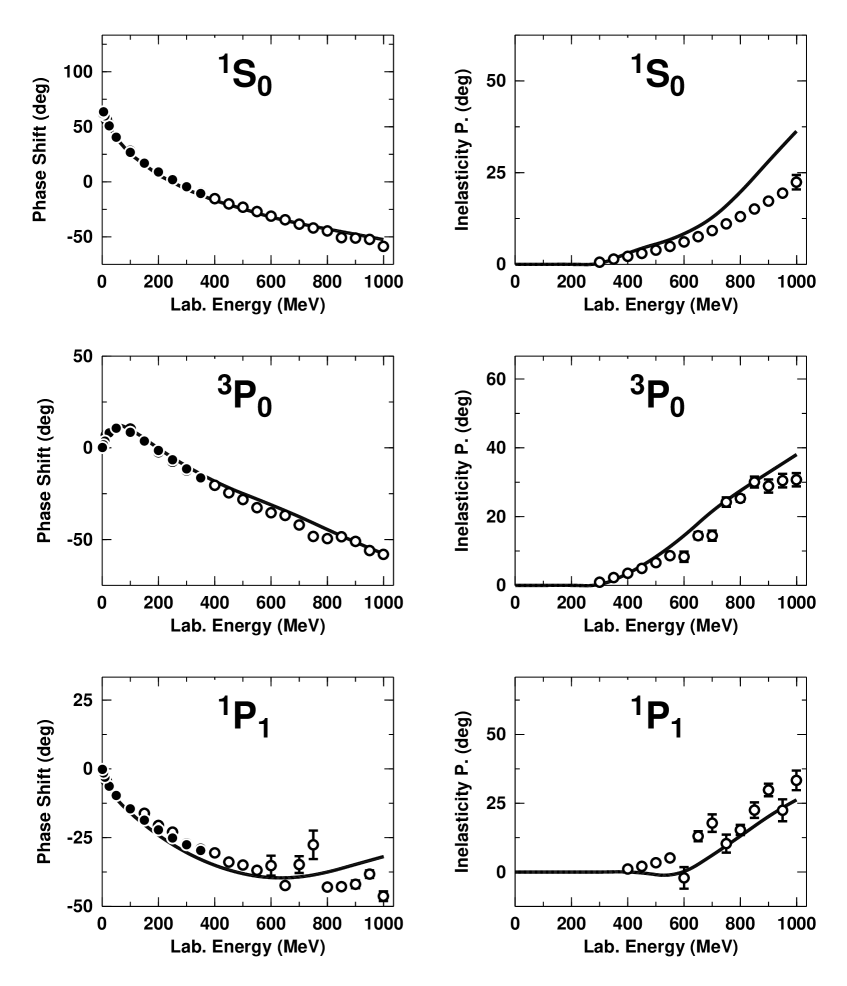
FIG. 3.: Phase shifts and inelasticity parameters of $NN$ scattering below 1 GeV laboratory energy. The solid curve represents the predictions by the model described in Sec. II. The solid dots show the Nijmegen multi-energy $np$ phase shift analysis [52], and the open circles are the GWU (formerly VPI) single-energy $np$ analysis SP03  [53]. Arndt-Roper conventions are used for the phase parameters [54].

Fig. 3 continued.

Fig. 3 continued.

Fig. 3 continued.

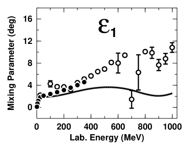
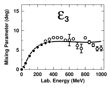
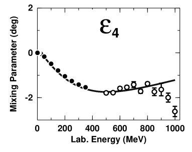
FIG. 4.: Mixing parameters for $J\leq 4$ and laboratory energies below 1 GeV. The solid curve represents the prediction by the model described in Sec. II. The solid dots show the results from the Nijmegen multi-energy $np$ analysis [52], and the open circles are the GWU (formerly VPI) single-energy $np$ analysis SP03  [53].

FIG. 5.: Total cross section (solid line) and total elastic cross section (dashed line) as predicted by the relativistic meson model presented in Sec. II. The experimental data for total cross sections are represented by solid symbols, while open symbols show the elastic cross section data.

FIG. 6.: Total cross section (solid line) and total elastic cross section (dashed line) as predicted by the relativistic meson model as modified in Sec. III. Data as in Fig. 5.

FIG. 7.: Observables of $pp$ scattering as denoted for five energies between 400 and 2500 MeV lab. energies. The dashed curve represents the predictions by the model of Sec. II, while the solid curve includes the modifications of Sec. III. The dotted curve is based upon the the GWU (formerly VPI) phase shift analysis SP03. Data from Refs. [33, 34, 35].

Fig. 7 continued.

FIG. 8.: The solid curve represents the prediction by a variation of our model that yields an improved fit of $A_{N}$ at 1.8 GeV. The dashed curve is identical to the solid curve of Fig. 7. Dotted curve and data as in Fig. 7.

Fig. 8 continued.