Quasielastic neutrino-nucleus scattering

Abstract

We study the sensitivity of neutral-current neutrino-nucleus scattering to the strange-quark content of the axial-vector form factor of the nucleon. A model-independent formalism for this reaction is developed in terms of eight nuclear structure functions. Taking advantage of the insensitivity of the ratio of proton $(\nu,\nu^{\prime}p)$ to neutron $(\nu,\nu^{\prime}n)$ yields to distortion effects, we compute all structure functions in a relativistic plane wave impulse approximation approach. Further, by employing the notion of a bound-state nucleon propagator, closed-form, analytic expressions for all nuclear-structure functions are developed in terms of an accurately calibrated relativistic mean-field model. Using a strange-quark contribution to the axial-vector form factor of $g_{A}^{s}\!=\!-0.19$, a significant enhancement in the proton-to-neutron yields is observed relative to one with $g_{A}^{s}\!=\!0$.

I Introduction

Neutrino physics has established itself at the forefront of current theoretical and experimental research in astro, nuclear and particle physics. While neutrino-oscillation experiments, which are presently evolving from the discovery to the precision phase, will remain at the center of most investigations, a variety of other interesting (non-oscillation) physics topics may be studied in parallel. A prime example of such a paradigm is the recently commissioned MiniBooNE experiment at Fermilab. While MiniBooNE’s primary goal is to confirm the neutrino-oscillation experiment at the Liquid Scintillator Neutrino Detector (LSND) at the Los Alamos National Laboratory Athanassopoulos et al. (1995) this unique facility is ideal for the study of supernova neutrinos, neutrino-nucleus scattering, and hadronic structure. In this contribution we focus on hadronic structure, in part as a response to the Fermilab Intense Neutrino Scattering Experiment (FINeSE) initiative that aims to measure the strange-quark contribution to the spin of the proton via neutral-current elastic scattering Potterveld et al. (2002).

A measurement of the spin asymmetry in deep-inelastic scattering of polarized muons on polarized protons by the European Muon Collaboration Ashman et al. (1989) revealed a disagreement with the Ellis-Jaffe sum rule Ellis and Jaffe (1974) in an approach that assumed that only up and down quarks (and antiquarks) contribute to the proton spin. This was one of the first indications that hidden flavor in the nucleon may play an important role in the determination of the spin structure of the proton. Experimentally, the spin structure of the proton is also accessible via parity-violating electron scattering. Unfortunately, large radiative corrections Musolf and Holstein (1990); Musolf et al. (1994) as well as nuclear-structure effects Horowitz and Piekarewicz (1993) hinder the extraction of strange-quark information. A complementary experimental technique that may be used effectively to study the spin structure of the proton is elastic neutrino-proton scattering. The advantages of neutral-current neutrino-proton scattering over parity-violating electron scattering and deep-inelastic scattering are well documented in the literature Kaplan and Manohar (1988); Potterveld et al. (2002). Two notable examples are: (i) the insensitivity of the extraction of the strange-quark contribution to the use of (broken) SU(3)-flavor symmetry Kaplan and Manohar (1988) and (ii) the absence of radiative corrections in neutral-current neutrino scattering Musolf et al. (1994); Potterveld et al. (2002). The quark structure of the nucleon may be investigated in a particularly clean fashion by evaluating matrix elements of suitable quark-current operators between single nucleon states Musolf et al. (1994); Anselmino et al. (1995); Lampe and Reya (2000); Alberico et al. (2002). This is because quark-current operators may be written in terms of the fundamental couplings of the quarks to the $Z^{0}$-boson, which are fully prescribed in the Standard Model. Further, the weak neutral current of the nucleon may be parametrized on completely general ground in terms of two vector and one axial form factors (an additional induced pseudoscalar form factor is present but its contribution vanishes in the limit of a zero neutrino mass). In particular, the axial-vector form factor may be split into a non-strange contribution, that may be determined from nuclear beta decay, and a strange contribution proportional to the fraction of the nucleon spin carried by the strange quarks Garvey et al. (1993a). Thus, the axial-vector form factor is crucial to understanding the role played by strange quarks in determining the properties of the proton and represents the main focus of this contribution.

A measurement of neutrino-proton and antineutrino-proton elastic scattering at the Brookhaven National Laboratory (BNL) reported a non-zero value for the strange form factors of the nucleon Ahrens et al. (1987). However, these results must be treated with caution as the value of the axial mass $M_{A}$ and $g_{A}^{s}$ are strongly correlated Garvey et al. (1993a). Another point of concern in the BNL experiment was that 80% of the events involved the scattering of a neutrino off carbon atoms and only 20% where from free protons. Before any firm conclusion may be reached, it is therefore necessary to understand nuclear-structure effects. Unfortunately, scattering off a nucleus introduces its own complications. These include: (i) questions concerning finite-density effects, such as possible modifications to the nucleon properties in the nuclear medium and (ii) conventional nuclear-structure effects, such as binding-energy corrections and Fermi motion. The first relativistic description of neutrino-nucleus scattering addressing these complications was presented in Ref. Horowitz et al. (1993), where the authors employed a relativistic Fermi-gas model for the target nucleus. Nuclear-structure effects were further investigated in Ref. Barbaro et al. (1996) by considering, in addition to a relativistic Fermi-gas model, a description of the bound nucleon in terms of harmonic oscillator wavefunctions. In general it was found that nuclear-structure effects and final-state interactions Garvey et al. (1993b) can have a substantial effect on the individual cross sections. However, as originally suggested in Ref. Garvey et al. (1992), the ratio of proton to neutron yields is largely insensitive to these effects Horowitz et al. (1993); Alberico et al. (1997).

In this work we also present a relativistic description of neutrino-nucleus scattering, but employing bound-state wavefunctions obtained from an accurately calibrated mean-field model Lalazissis et al. (1997). Further, the impulse approximation is assumed, that is, the neutrino-nucleon interaction is assumed unchanged in the nuclear medium. Finally, as the ultimate aim of this project is to compute ratios of cross sections, distortion effects on the ejectile nucleon will be neglected. As we will show later, this leads to a great simplification in the calculation of all relevant quantities. The paper has been organized as follows. The formalism is presented in Sec. II, followed by results and conclusions in Sec. III and Sec. IV, respectively.

II Formalism

In this section the formalism for the relativistic description of (neutral-current) neutrino-nucleus scattering will be presented. In particular, it will be shown in Sec. II.1 that the cross section can be written as a contraction between leptonic and hadronic tensors. In turn, by relying exclusively on fundamental principles, the hadronic tensor will be decomposed in terms of a set of invariant structure functions (see Sec II.2). Thus, the formalism is model-independent. Yet to determine the structure function, and ultimately the cross section, one must rely on a model. This will be discussed in Sec. II.3.

II.1 Cross section in terms of leptonic and hadronic tensors

Due to the short-range nature of the weak interaction, the one-boson exchange approximation provides an excellent description of neutrino-nucleus scattering. This results in a cross section that cleanly separates (or factorizes) into leptonic and hadronic components. The kinematics of the process is depicted in Fig. 1. Here the initial and final neutrino four-momenta are denoted by $k$ and $k^{\prime}$, respectively. Further, the reaction proceeds via the exchange of a virtual $Z^{0}$-boson with four-momentum $q$. The target and residual nucleus have four-momenta denoted by $P$ and $P^{\prime}$, respectively. Finally, the ejectile proton has four-momentum $p^{\prime}$ and spin component $s^{\prime}$.

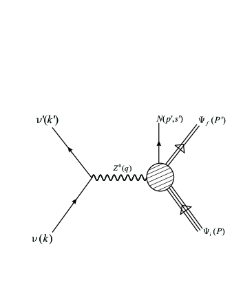
Figure 1: Lowest-order Feynman diagram for the knockout of a bound nucleon via neutral-current neutrino-nucleus scattering

The differential cross section can now be defined in terms of these kinematic variables and the transition matrix element ${\cal M}$ as follows:

$$d\sigma = \displaystyle\frac{(2\pi)^{4}\,\delta(k+P-k^{\prime}-p^{\prime}-P^{\prime}\,)}{|{\bf v}_{1}-{\bf v}_{2}\,|}\,\displaystyle\frac{d^{3}k^{\prime}}{(2\pi)^{3}}\;\displaystyle\frac{d^{3}p^{\prime}}{(2\pi)^{3}}\;\displaystyle\frac{d^{3}P^{\prime}}{(2\pi)^{3}}\;|{\cal M}|^{2}\;,$$ (1)

where ${\bf v}_{1}-{\bf v}_{2}$ denotes the initial relative velocity. The transition-matrix element contains all the dynamical information about the reaction and is given, in the conventions of Ref. Musolf et al. (1994), by

$$-i{\cal M}=\left(\overline{\nu}({\bf k}^{\prime})\left[\frac{igM_{Z}}{4M_{W}}(\gamma^{\mu}\!-\!\gamma^{\mu}\gamma^{5})\right]\nu({\bf k})\right)iD_{\mu\nu}(q)\left(\langle p^{\prime},\!s^{\prime};\Psi_{f}(P^{\prime})\Big{|}\frac{igM_{Z}}{4M_{W}}\hat{J}^{\nu}(q)\Big{|}\Psi_{i}(P)\rangle\right)\;.$$ (2)

Note that in Eq. (2) the initial and final nuclear states are denoted by $\Psi_{i}(P)$ and $\Psi_{f}(P^{\prime})$, respectively. Further, $g$ is the weak coupling constant and $\hat{J}_{\mu}(q)$ is the weak nuclear current operator, which contains both vector and axial-vector components. Finally, as only low momentum transfer ($|q^{2}|\ll M_{Z}^{2}$) scattering will be considered, the following replacement is valid:

$$D_{\mu\nu}(q)=\frac{-g_{\mu\nu}+q_{\mu}q_{\nu}/M_{Z}^{2}}{q^{2}-M_{Z}^{2}}\longrightarrow\frac{g_{\mu\nu}}{M_{Z}^{2}}.$$ (3)

This allows the transition matrix element to be written as

$${\cal M}=\frac{G_{F}}{2\sqrt{2}}\left[\overline{\nu}({\bf k}^{\prime})(\gamma^{\mu}\!-\!\gamma^{\mu}\gamma^{5})\nu({\bf k})\right]\left[\langle p^{\prime},\!s^{\prime};\Psi_{f}(P^{\prime})\Big{|}\hat{J}^{\nu}(q)\Big{|}\Psi_{i}(P)\right]\;.$$ (4)

Note that $G_{F}$ is the Fermi constant for muon decay which is given by

$$G_{F}=\frac{g^{2}}{4\sqrt{2}M_{W}^{2}}\simeq 1.166\times 10^{-5}~{}{\rm GeV}^{-2}\;.$$ (5)

In Eq. (2) and throughout this work plane-wave Dirac spinors are defined as follows:

$${\cal U}({\bf k},s)=\sqrt{\frac{E_{k}+M}{2E_{k}}}\left(\begin{array}[]{c}1\\ \displaystyle{\frac{\mbox{\boldmath$\sigma$}\cdot{\bf k}}{E_{k}+M}}\end{array}\right)\chi_{s}\;,\quad\Big{(}E_{k}\equiv\sqrt{{\bf k}^{2}+M^{2}}\Big{)}\;.$$ (6)

Note that the above definition corresponds to the normalization

$${\cal U}^{\dagger}({\bf k},s){\cal U}({\bf k},s)=\delta_{ss^{\prime}}\;.$$ (7)

This (non-covariant) normalization is motivated by the standard choice adopted for bound-state spinors (see Sec. II.3 and Ref. Serot and Walecka (1986)) which is given by

$$\int{\cal U}_{\alpha}^{\dagger}({\bf r})\,{\cal U}_{\alpha}({\bf r})\,d{\bf r}=1\;.$$ (8)

For (massless) neutrinos in the laboratory frame the initial flux factor in Eq. (1) is equal to one. Substitution of the above relations into Eq. (1) leads to the following expression for the differential cross section:

$$d\sigma=\frac{G_{F}^{2}}{8}(2\pi)^{4}\delta(k+P-k^{\prime}-p^{\prime}-P^{\prime})\displaystyle\frac{d^{3}{\bf k}^{\prime}}{(2\pi)^{3}}\;\displaystyle\frac{d^{3}{\bf p}^{\prime}}{(2\pi)^{3}}\;\displaystyle\frac{d^{3}{\bf P}^{\prime}}{(2\pi)^{3}}\;\ell_{\mu\nu}W^{\mu\nu}\;,$$ (9)

where the leptonic tensor is given by

$$\ell^{\mu\nu}=\Big{[}\overline{\nu}({\bf k}^{\prime})(\gamma^{\mu}\!-\!\gamma^{\mu}\gamma^{5})\nu({\bf k})\Big{]}\Big{[}\overline{\nu}({\bf k}^{\prime})(\gamma^{\nu}\!-\!\gamma^{\nu}\gamma^{5})\nu({\bf k})\Big{]}^{*}$$ (10)

while the hadronic tensor by

$$W^{\mu\nu}=\left[\langle p^{\prime},\!s^{\prime};\Psi_{f}(P^{\prime})\Big{|}\hat{J}^{\mu}(q)\Big{|}\Psi_{i}(P)\right]\left[\langle p^{\prime},\!s^{\prime};\Psi_{f}(P^{\prime})\Big{|}\hat{J}^{\nu}(q)\Big{|}\Psi_{i}(P)\right]^{*}\;.$$ (11)

The integral over ${\bf P}^{\prime}$ may be performed using the spatial part of the Dirac delta function. This fixes the three-momentum of the residual nucleus to be

$${\bf P}^{\prime}={\bf k}-{\bf k}^{\prime}-{\bf p}^{\prime}+{\bf P}\mathop{\longrightarrow}_{\rm lab}{\bf q}-{\bf p}^{\prime}\;,$$ (12)

where ${\bf q}\!\equiv\!{\bf k}\!-\!{\bf k}^{\prime}$ is the three-momentum transfer to the nucleus. The differential cross section can now be written as

$$d\sigma=\frac{G_{F}^{2}}{8(2\pi)^{5}}d^{3}{\bf k}^{\prime}d^{3}{\bf p}^{\prime}\delta(E_{k}\!+\!M_{A}\!-\!E_{k^{\prime}}\!-\!E_{p^{\prime}}\!-\!E_{P^{\prime}})\ell_{\mu\nu}W^{\mu\nu}\;.$$ (13)

II.2 Differential cross section in terms of nuclear structure functions

In Sec. II.1 it has been shown that the differential cross for nucleon knockout in neutrino-nucleus scattering involves the contraction between the leptonic tensor $\ell_{\mu\nu}$ [Eq. (10)] and the hadronic tensor $W^{\mu\nu}$ [Eq. (11)]. In this section both of these quantities will be calculated in a model-independent way by introducing a suitable set of nuclear structure functions.

Starting from Eq. (10) it follows that the leptonic tensor may be written as

$$\ell^{\mu\nu} = {\rm Tr}\left[(\gamma^{\mu}\!-\!\gamma^{\mu}\gamma^{5})\Big{(}\nu({\bf k})\overline{\nu}({\bf k})\Big{)}(\gamma^{\nu}\!-\!\gamma^{\nu}\gamma^{5})\Big{(}\nu({\bf k}^{\prime})\overline{\nu}({\bf k}^{\prime})\Big{)}\right]$$ (14)

$$= \frac{2}{kk^{\prime}}\Big{[}k^{\mu}k^{\prime\nu}+k^{\prime\mu}k^{\nu}-g^{\mu\nu}k\cdot k^{\prime}+ih\epsilon^{\mu\nu\alpha\beta}k_{\alpha}k^{\prime}_{\beta}\Big{]}\;,$$

where we made use of Eq. (6) to write

$$\nu({\bf k})\overline{\nu}({\bf k})=\frac{\hbox to0.0pt{/\hss}k}{2k}\left[\frac{1}{2}(1-h\gamma^{5})\right]\;,\quad(k\equiv{|{\bf k}|})\;.$$ (15)

Note that in the above expressions $h\!=\!-1$ and $h\!=\!+1$ refer to left-handed neutrinos and right-handed antineutrinos, respectively. For later convenience, the leptonic tensor can now be separated into a symmetric and an antisymmetric part. That is,

$$\ell^{\mu\nu}\equiv\ell_{S}^{\mu\nu}+\ell_{A}^{\mu\nu}\;,$$ (16)

where

$$\ell_{S}^{\mu\nu} = \frac{2}{kk^{\prime}}(k^{\mu}k^{\prime\nu}+k^{\prime\mu}k^{\nu}-g^{\mu\nu}k\cdot k^{\prime})\;,$$ (17a)

$$\ell_{A}^{\mu\nu} = \frac{2}{kk^{\prime}}ih\epsilon^{\mu\nu\alpha\beta}k_{\alpha}k^{\prime}_{\beta}\;.$$ (17b)

Note that all remnants of the neutrino helicity resides in the term containing the antisymmetric Levi-Civita tensor. It is only this antisymmetric component of the leptonic tensor that is sensitive to the difference between an incident neutrino or antineutrino beam. It then follows from Eq. (17), as the weak neutral currents is conserved for massless neutrinos, that

$$q_{\mu}\ell^{\mu\nu}=\ell^{\mu\nu}q_{\nu}=0\;,$$ (18)

where $q^{\mu}\!\equiv\!(\omega,{\bf q})\!=\!(k^{\mu}\!-\!k^{\prime\mu})$ is the four-momentum transfer to the nucleus.

The hadronic tensor is an extremely complicated object as in principle exact many-body wave functions and operators must be used. Yet it follows from Eq. (11) that for unpolarized nucleon emission the hadronic tensor is only a function of three independent four-momenta: $q^{\mu}$, $P^{\mu}$ and $p^{\prime\mu}$, as the four-momentum of the recoiling nucleus $P^{\prime\mu}$ is fixed by four-momentum conservation. The hadronic tensor can therefore be parametrized in terms of a basis constructed from the following five tensors: $\left\{q^{\mu},P^{\mu},p^{\prime\prime\mu},g^{\mu\nu},\epsilon^{\mu\nu\alpha\beta}\right\}$. This is analogous to the case of electron scattering but now we are no longer allowed to invoke either parity invariance or current conservation, as the weak interaction violates parity and the axial-vector current is not conserved. We start by separating the hadronic tensor into symmetric and antisymmetric components. That is,

$$W^{\mu\nu}\equiv W_{S}^{\mu\nu}+W_{A}^{\mu\nu}\;.$$ (19)

Using the above-mentioned basis the individual components may be written as follows:

$$W_{S}^{\mu\nu} = W_{1}g^{\mu\nu}+W_{2}q^{\mu}q^{\nu}+W_{3}P^{\mu}P^{\nu}+W_{4}\,p^{\prime\mu}p^{\prime\nu}$$ (20a)

$$+ W_{5}(q^{\mu}P^{\nu}\!+\!P^{\mu}q^{\nu})+W_{6}(q^{\mu}p^{\prime\nu}\!+p^{\prime\mu}q^{\nu})+W_{7}(P^{\mu}p^{\prime\nu}\!+p^{\prime\mu}P^{\nu})\;,$$

$$W_{A}^{\mu\nu} = W_{8}(q^{\mu}P^{\nu}\!-\!P^{\mu}q^{\nu})+W_{9}(q^{\mu}p^{\prime\nu}\!-p^{\prime\mu}q^{\nu})+W_{10}(P^{\mu}p^{\prime\nu}\!-p^{\prime\mu}P^{\nu})$$ (20b)

$$+ W_{11}\epsilon^{\mu\nu\alpha\beta}q_{\alpha}P_{\beta}+W_{12}\epsilon^{\mu\nu\alpha\beta}q_{\alpha}p^{\prime}_{\beta}+W_{13}\epsilon^{\mu\nu\alpha\beta}P_{\alpha}p^{\prime}_{\beta}\;.$$

Note that all structure functions are functions of the four Lorentz-invariant quantities, $q^{\mu}q_{\mu}\!\equiv\!-Q^{2}$, $q\cdot P$, $q\cdot p^{\prime}$, and $P\cdot p^{\prime}$. The hadronic tensor for the $(\nu,\nu^{\prime}p)$ [or $(\nu,\nu^{\prime}n)$] reaction contains thirteen independent structure functions. Contrast this, for example, to the hadronic tensor for $(e,e^{\prime}p)$ which is fully written in terms of only five structure functions Picklesimer et al. (1985).

We now proceed to evaluate the contraction of the leptonic tensor with the hadronic tensor. First, we introduce the following definition:

$${\cal F}(k,k^{\prime};P,p^{\prime})\equiv\left(\frac{4}{kk^{\prime}}\right)^{-1}\ell_{\mu\nu}W^{\mu\nu}={\cal F}_{S}(k,k^{\prime};P,p^{\prime})+{\cal F}_{A}(k,k^{\prime};P,p^{\prime})\;,$$ (21)

where ${\cal F}_{S}$ and ${\cal F}_{A}$ are defined in terms of the symmetric and antisymmetric components of the leptonic and hadronic tensors, respectively. That is,

$${\cal F}_{S}(k,k^{\prime};P,p^{\prime}) \equiv \left(\frac{4}{kk^{\prime}}\right)^{-1}\ell_{\mu\nu}^{S}W^{\mu\nu}_{S}$$ (22a)

$$= \Bigg{(}-W_{1}(k\cdot k^{\prime})+W_{3}\left[(k\cdot P)(k^{\prime}\cdot P)+\frac{M_{A}}{2}^{2}(k\cdot k^{\prime})\right]$$

$$+ W_{4}\left[(k\cdot p^{\prime})(k^{\prime}\cdot p^{\prime})+\frac{M_{N}^{2}}{2}(k\cdot k^{\prime})\right]$$

$$+ W_{7}\Big{[}(k\cdot P)(k^{\prime}\cdot p^{\prime})+(k\cdot p^{\prime})(k^{\prime}\cdot P)-(k\cdot k^{\prime})(P\cdot p^{\prime})\Big{]}\Bigg{)}\;,$$

$${\cal F}_{A}(k,k^{\prime};P,p^{\prime}) \equiv \left(\frac{4}{kk^{\prime}}\right)^{-1}\ell_{\mu\nu}^{A}W^{\mu\nu}_{A}$$ (22b)

$$= ih\Bigg{(}W_{10}\epsilon^{\mu\nu\alpha\beta}k_{\mu}k^{\prime}_{\nu}P_{\alpha}p^{\prime}_{\beta}+W_{11}(k\cdot k^{\prime})\Big{(}k\cdot P+k^{\prime}\cdot P\Big{)}$$

$$+ W_{12}(k\cdot k^{\prime})\Big{(}k\cdot p^{\prime}+k^{\prime}\cdot p^{\prime}\Big{)}$$

$$+ W_{13}\Big{[}(k\cdot p^{\prime})(k^{\prime}\cdot P)-(k\cdot P)(k^{\prime}\cdot p^{\prime})\Big{]}\Bigg{)}\;.$$

Note that as a result of current conservation, only eight of the original thirteen structure functions survived the contraction [see Eq. (18)]. Further, an interesting difference between neutrino and electron scattering can be seen from Eq. (22b). While for electron scattering one must prepare a polarized beam to sample the antisymmetric part of the hadronic tensor Picklesimer et al. (1985), for neutrinos the polarization happens by default. Eqs. (13), (22a), and (22b) comprise the principal results for this section. It is the most general structure possible for nucleon knockout in neutral-current neutrino-nucleus scattering. It shows that the differential cross section is completely determined by a set of eight structure functions multiplied by kinematical factors.

II.3 Model-dependent calculation of the cross section

In the previous section it was shown that the differential cross section is completely determined by a set of eight structure functions. These structure functions parametrize our ignorance about strong-interaction physics. In principle, these structure functions could be measured through a “super” Rosenbluth separation. In practice, however, this is beyond realistic expectations. Thus, it is not possible to proceed further without an explicit model of the hadronic vertex.

First, we focus on some “kinematical” approximations that are made in order to simplify the argument of the energy conserving delta function in Eq. (13). In the laboratory frame the total energy of the residual nucleus is given by

$$E_{P^{\prime}}=\sqrt{{\bf P}^{2}+M_{A-1}^{2}}=\sqrt{({\bf q}-{\bf p}^{\prime})^{2}+M_{A-1}^{2}}\approx M_{A-1}\;,$$ (23)

where the last approximation follows in the limit of no recoil corrections. Further, it is assumed that the energy transfer to the nucleus satisfies

$$\omega=k-k^{\prime}=E_{p^{\prime}}-E_{B}\;,$$ (24)

where $E_{B}$ is the energy of the struck nucleon. This implies that

$$E_{P^{\prime}}=M_{A}-E_{B}\;,$$ (25)

and justifies the following replacement in Eq. (13):

$$\delta(E_{k}\!+\!M_{A}\!-\!E_{k^{\prime}}\!-\!E_{p^{\prime}}\!-\!E_{P^{\prime}})\longrightarrow\delta(k\!-\!k^{\prime}\!-\!E_{p^{\prime}}\!+\!E_{B})\;.$$ (26)

Note that we have defined $E_{k}\!=\!|{\bf k}|\!\equiv\!k$ and $E_{k^{\prime}}\!=\!|{\bf k}^{\prime}|\!\equiv\!k^{\prime}$.

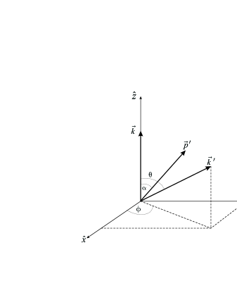
Figure 2: Coordinate axes used to define the angles $\alpha$, $\theta$ and $\phi$.

Consider now the coordinate system shown in Fig. 2 where the incoming neutrino defines the $\hat{\bf z}$-axis. The outgoing nucleon is detected at a scattering angle $\alpha$ relative to the $\hat{\bf z}$-axis, while the outgoing neutrino, assumed undetected, has polar and azimuthal angles $\theta$ and $\phi$, respectively. The following relations are therefore valid:

$$d^{3}{\bf k}^{\prime}=k^{\prime 2}\sin\theta dk^{\prime}d\theta d\phi\quad{\rm and}\quad d^{3}{\bf p}^{\prime}=2\pi p^{\prime}E_{p^{\prime}}dE_{p^{\prime}}d(\cos\alpha)\;.$$ (27)

As the outgoing neutrino will remain undetected, one must integrate over $k^{\prime}$, $\theta$ and $\phi$. Using Eqs. (26) and (27) the following expression for the differential cross section [Eq. (13)] is obtained:

$$\frac{d^{2}\sigma}{dE_{p^{\prime}}d(\cos\alpha)}=\left(\frac{G_{F}^{2}}{32\pi^{4}}\right)\left(\frac{|{\bf k}^{\prime}||{\bf p}^{\prime}|E_{p^{\prime}}}{|{\bf k}|}\right)\int_{0}^{\pi}\sin\theta d\theta\int_{0}^{2\pi}d\phi\,{\cal F}(k,k^{\prime};P,p^{\prime})\;,$$ (28)

where the energy conserving delta function constrains the energy of the outgoing neutrino to $|{\bf k}^{\prime}|\!=\!|{\bf k}|\!+\!E_{B}\!-\!E_{p^{\prime}}$.

What remains now is to provide an explicit form for the eight independent structure functions introduced in the previous section. It follows from Eq. (4) that the dynamical information on the hadronic vertex is contained in the following matrix element (and its complex conjugate):

$$J^{\mu}=\langle p^{\prime},\!s^{\prime};\Psi_{f}(P^{\prime})\Big{|}\hat{J}^{\mu}(q)\Big{|}\Psi_{i}(P)\rangle\;.$$ (29)

To obtain a tractable form for this extremely complicated object we rely on the approximations depicted in Fig. 3, that we now address in detail.

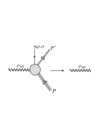
Figure 3: Graphical representation of the approximation employed at the hadronic vertex to obtain a tractable form for the matrix element given in Eq. (29).

First, it is assumed that the $Z^{0}$-boson couples to a single bound nucleon. This neglects two- and many-body components of the current operator. Second, it is assumed that the detected nucleon is the one to which the virtual boson couples to. This neglects two- and many-body rescattering processes. Finally, we neglect final-state interactions (distortions) of the ejected nucleon. While many similar treatments incorporate distortion effects on the ejectile (see for example Ref. Picklesimer et al. (1985) in the case of electron scattering) concentrating on ratios of cross sections makes the formalism largely insensitive to distortion effects Garvey et al. (1993a). This will render the hadronic tensor analytic. Incorporating the above simplifications yields a hadronic matrix element of the following simple form:

$$J^{\mu}=\overline{\cal U}({\bf p}^{\prime},s^{\prime})\hat{J}^{\mu}(q){\cal U}_{\alpha}({\bf p}_{m})\;,$$ (30)

where $\alpha$ represents a collection of quantum numbers and ${\bf p}_{m}\!\equiv\!{\bf p}^{\prime}\!-\!{\bf q}$ is the missing momentum. Note that the bound-state wavefunction is given by

$${\cal U}_{\alpha}({\bf p})\equiv{\cal U}_{E\kappa m}({\bf p})=\frac{4\pi}{p}(-i)^{l}\left(\begin{array}[]{c}g_{E\kappa}(p)\\ f_{E\kappa}(p)(\mbox{\boldmath$\sigma$}\cdot\hat{\bf p})\end{array}\right){\cal Y}_{\kappa m}(\hat{\bf p})\;.$$ (31)

Here $E$ is the bound-state energy, $\kappa$ the (generalized) angular momentum, and $m$ the spin projection. Further, $g_{E\kappa}(p)$ and $f_{E\kappa}(p)$ are Fourier transforms of the upper and lower components of the bound-state wavefunction, respectively Gardner and Piekarewicz (1994).

The impulse approximation is now invoked by assuming that the weak neutral current for a nucleon in the nuclear medium retains its free-space form. That is,

$$\hat{J}_{\mu}\equiv\hat{J}_{\mu}^{\rm NC}-\hat{J}_{\mu 5}^{\rm NC}=\widetilde{F}_{1}(Q^{2})\gamma_{\mu}+i\widetilde{F}_{2}(Q^{2})\sigma_{\mu\nu}\frac{q^{\nu}}{2M}-\widetilde{G}_{A}(Q^{2})\gamma_{\mu}\gamma_{5}\;.$$ (32)

Here $\widetilde{F}_{1}$ and $\widetilde{F}_{2}$ are Dirac and Pauli vector form factors, respectively and $\widetilde{G}_{A}$ is the axial form factor. The additional induced pseudoscalar form factor (proportional to $q_{\mu}$) does not contribute to (massless) neutrino scattering and will be neglected henceforth. The two vector form factors may be decomposed in terms of the usual electromagnetic Dirac and Pauli form factors, plus a yet undetermined strange-quark contribution. Similarly, the axial vector form factor consists of a purely isovector contribution, that may be determined from Gamow-Teller $\beta$-decay rates, and a purely isoscalar strange-quark contribution. It is the aim of this contribution to explore the sensitivity of neutral-current neutrino-nucleus scattering to the strange-quark contribution to the axial form factor. A detailed discussion of the weak neutral current [Eq. (32)] is given in Appendix A.

It is now possible, using Eq. (30), to explicitly calculate the hadronic tensor defined in Eq. (11). Assuming that the spin of the outgoing nucleon is not detected, the hadronic tensor may be written as

$$W^{\mu\nu} = \sum_{s^{\prime}}\sum_{m}\left[\overline{{\cal U}}({\bf p}^{\prime},s^{\prime})\hat{J}^{\mu}(q){\cal U}_{\alpha,m}({\bf p}_{m})\right]\left[\overline{{\cal U}}({\bf p}^{\prime},s^{\prime})\hat{J}^{\nu}(q){\cal U}_{\alpha,m}({\bf p}_{m})\right]^{*}$$ (33)

$$= {\rm Tr}\left[\hat{J}^{\mu}(q)S_{\alpha}({\bf p}_{m})\hat{\bar{J}}^{\nu}(q)S({\bf p}^{\prime})\right]\;,$$

where $\hat{\bar{J}}^{\nu}\!=\!\gamma^{0}(\hat{J}^{\nu})^{\dagger}\gamma^{0}$. The normalization used in Eq. (7) implies that the standard (on-shell) Feynman propagator is given by

$$S({\bf p}^{\prime})=\sum_{s^{\prime}}{\cal U}({\bf p}^{\prime},s^{\prime})\,\overline{{\cal U}}({\bf p}^{\prime},s^{\prime})=\frac{\hbox to0.0pt{/\hss}p^{\prime}+M}{2E_{{\bf p}^{\prime}}}\;.$$ (34)

Moreover, it has been shown in Ref. Gardner and Piekarewicz (1994) that the following simple identity is valid even in the case of a bound-state spinor:

$$S_{\alpha}({\bf p})\equiv\sum_{m}{\cal U}_{\alpha,m}({\bf p})\,\overline{\cal U}_{\alpha,m}({\bf p})=(2j+1)({\hbox to0.0pt{/\hss}{p}}_{\alpha}+M_{\alpha})\;.$$ (35)

Note that in the above equation for the “bound-state” propagator mass-, energy-, and momentum-like quantities have been introduced. These are given by

$$M_{\alpha} = \left(\frac{\pi}{p^{2}}\right)\Big{[}g_{\alpha}^{2}(p)-f_{\alpha}^{2}(p)\Big{]}\;,$$ (36a)

$$E_{\alpha} = \left(\frac{\pi}{p^{2}}\right)\Big{[}g_{\alpha}^{2}(p)+f_{\alpha}^{2}(p)\Big{]}\;,$$ (36b)

$${\bf p}_{\alpha} = \left(\frac{\pi}{p^{2}}\right)\Big{[}2g_{\alpha}(p)f_{\alpha}(p)\hat{\bf p}\Big{]}\;,$$ (36c)

and satisfy the “on-shell relation”

$$p_{\alpha}^{2}=E_{\alpha}^{2}-{\bf p}_{\alpha}^{2}=M_{\alpha}^{2}\;.$$ (37)

It now follows from Eqs. (34) and (35) that the hadronic tensor may be written in the following simple form:

$$W^{\mu\nu}=\left(\frac{2j+1}{2E_{{\bf p}^{\prime}}}\right){\rm Tr}\left[\hat{J}^{\mu}(q)({\hbox to0.0pt{/\hss}{p}}_{\alpha}+M_{\alpha})\hat{\bar{J}}^{\nu}(q)(\hbox to0.0pt{/\hss}p^{\prime}+M)\right]\;.$$ (38)

The fact that the hadronic tensor may be expressed as a trace over Dirac matrices, despite the presence of the bound-state wave function, greatly simplifies the calculation. It is important to note, however, that this enormous simplification would have been lost if distortion effects would have been incorporated in the propagation of the emitted nucleon. The emphasis on computing ratios of cross sections is the main justification behind this simplification. We now obtain

$$W^{\mu\nu} = \left(\frac{2j+1}{2E_{{\bf p}^{\prime}}}\right)\left[\widetilde{W}_{1}g^{\mu\nu}+\widetilde{W}_{2}\left(p^{\prime\mu}p_{\alpha}^{\nu}+p_{\alpha}^{\mu}p^{\prime\nu}\right)+\widetilde{W}_{3}\left(q^{\mu}p_{\alpha}^{\nu}+p_{\alpha}^{\mu}q^{\nu}\right)+\widetilde{W}_{4}\left(q^{\mu}p^{\prime\nu}+p^{\prime\mu}q^{\nu}\right)+\right.$$ (39)

$$\left.\hskip 56.9055pt\widetilde{W}_{5}q^{\mu}q^{\nu}+\widetilde{W}_{6}\epsilon^{\mu\nu\sigma\lambda}p_{\alpha,\sigma}p_{\lambda}^{\prime}+\widetilde{W}_{7}\epsilon^{\mu\nu\sigma\lambda}p_{\alpha,\sigma}q_{\lambda}+\widetilde{W}_{8}\epsilon^{\mu\nu\sigma\lambda}p_{\sigma}^{\prime}q_{\lambda}\right]\;.$$

All components of the hadronic tensor are given in terms of relatively simple expressions that have been collected in Appendix B. These model-dependent structure functions may be related to the model-independent ones [see Eqs. (20a) and (20b)] as has been shown in Appendix B. This concludes the formalism for neutral-current neutrino-nucleus scattering. The explicit forms of the structure functions given in the appendix can now be used to evaluate the differential cross section defined in Eq. (28).

III Results

In Ref. Horowitz et al. (1993) the strange-quark content of the nucleon was studied via neutrino-nucleus scattering by using a relativistic Fermi gas model of the target nucleus. This amounts to averaging the free neutrino-nucleon cross section over a sharp momentum distribution for the struck nucleon. In this work we improve on the above description by employing bound-nucleon wavefunctions obtained from a relativistic mean-field approximation to the accurately calibrated NL3 model of Ref. Lalazissis et al. (1997). To quantify the impact of this improvement we display in Figs. 4 to 6 the double differential cross section $d^{2}{\sigma}/dE_{p^{\prime}}d(\cos\alpha)$ as a function of the ejectile nucleon kinetic energy $T_{p}$ and its scattering angle $\alpha$ in the laboratory frame. The incident neutrino energy has been fixed in these plots at 150, 500 and 1000 MeV, respectively. For illustration purposes—and only for these three graphs—the strange-quark contribution to the axial-vector form factor ($g_{A}^{s}$) has been neglected and only proton knockout from the $1p^{3/2}$ orbital of ¹²C is considered.

Figure 4: Double differential cross section $d^{2}\sigma/dEd(\cos\alpha)$ as a function of the outgoing proton laboratory kinetic energy $T_{p}$ and laboratory scattering angle $\alpha$. The calculation shown is for proton knockout from the $1p^{3/2}$ orbital of ¹²C at an incident neutrino energy of 150 MeV.

Figure 5: Double differential cross section $d^{2}\sigma/dEd(\cos\alpha)$ as a function of the outgoing proton laboratory kinetic energy $T_{p}$ and laboratory scattering angle $\alpha$. The calculation shown is for proton knockout from the $1p^{3/2}$ orbital of ¹²C at an incident neutrino energy of 500 MeV.

Figure 6: Double differential cross section $d^{2}\sigma/dEd(\cos\alpha)$ as a function of the outgoing proton laboratory kinetic energy $T_{p}$ and laboratory scattering angle $\alpha$. The calculation shown is for proton knockout from the $1p^{3/2}$ orbital of ¹²C at an incident neutrino energy of 1000 MeV.

For the lowest energy neutrinos the cross section displays a single well developed peak at low $T_{p}$ that monotonically decreases with increasing scattering angle $\alpha$. For $E_{\nu}\!=\!500$ MeV, our Fig. 5 may be compared directly to Fig. 1 of Horowitz and collaborators Horowitz et al. (1993). In particular, for a scattering angle of $\alpha\!=\!20^{\circ}$, our calculation (third curve along the $\alpha$ direction) also exhibits the characteristic double-humped structure. For larger values of $\alpha$ the peaks merge into one and the cross section develops a shape similar to that of $E_{\nu}\!=\!150$ MeV. Yet, an important difference between the two sets of calculations is that our cross section does not develop the sharp features displayed at small angles in Ref. Horowitz et al. (1993). This is due to the more realistic momentum distributions used in our calculations.

Next, we produce angle-integrated cross sections as a function of $T_{p}$. Figs. 7 and 8 display cross sections for the knockout of protons and neutrons, respectively. The long-dash–short-dashed line represents knockout from the $1s^{1/2}$ orbital while the dashed line from the $1p^{3/2}$ orbital of ¹²C; the solid line displays their sum. As before, calculations are shown for incident neutrino energies of 150, 500, and 1000 MeV, respectively. The cross sections at 150 MeV correspond to those shown in Figs. 4 and 5 of Ref. Horowitz et al. (1993). It has been shown in Ref. Horowitz et al. (1993) that binding-energy corrections (at 150 MeV) reduce the cross sections relative to their free Fermi-gas values by about 40%. Our cross sections (already summed over both occupied orbitals) are reduced even further. Note that while an average binding energy of 27 MeV has been used in Ref. Horowitz et al. (1993), our calculations include binding energies computed exactly within a mean-field approach. At the higher energies of 500 and 1000 MeV the cross sections display the same general trend as the one for 150 MeV, namely, a peak at a low value of $T_{p}$ and a “smooth” falloff with increasing $T_{p}$.

Figure 7: Differential cross section $d\sigma/dE$ as a function of the outgoing proton laboratory kinetic energy $T_{p}$. The dashed and long-dashed–short-dashed lines are for proton knockout from the $1p^{3/2}$ and $1s^{1/2}$ orbitals of ¹²C, respectively; the solid line represents their sum. The incident neutrino energy is taken to be $E_{k}$ = 150, 500 and 1000 MeV.

Figure 8: Differential cross section $d\sigma/dE$ as a function of the outgoing neutron laboratory kinetic energy $T_{p}$. The dashed and long-dashed–short-dashed lines are for neutron knockout from the $1p^{3/2}$ and $1s^{1/2}$ orbitals of ¹²C, respectively; the solid line represents their sum. The incident neutrino energy is taken to be $E_{k}$ = 150, 500 and 1000 MeV.

In Figs. 9 and 10 we examine the impact of a strange-quark contribution ($g_{A}^{s}$) to the axial form factor on the cross section. Following the discussions in Refs. Ahrens et al. (1987); Ashman et al. (1989); Horowitz et al. (1993) a value of $g_{A}^{s}\!=\!-\!0.19$ is adopted henceforth. Further, in all cases presented here strange-quark contributions to the weak vector form factors are ignored. The solid and dashed lines correspond to a zero and a non-zero value of $g_{A}^{s}$, respectively. In both figures we have summed over the $1s^{1/2}$ and the $1p^{3/2}$ orbitals of ¹²C. Because of the dominance of the axial-vector form factor (see discussion below) a non-zero value of $g_{A}^{s}$ increases the cross section for proton knockout, whereas for neutron knockout the cross section is decreased. These findings are consistent with those of Refs. Horowitz et al. (1993); Garvey et al. (1992).

Figure 9: Effect of a strange-quark contribution (of $g_{A}^{s}\!=\!-0.19$) to the axial-vector form factor on the differential cross section $d\sigma/dE$ as a function of the laboratory kinetic energy $T_{p}$ of the outgoing proton. The solid and dashed lines correspond to a zero and a non-zero value of $g_{A}^{s}$, respectively. In this figure we have summed over the $1s^{1/2}$ and $1p^{3/2}$ orbitals of ¹²C.

Figure 10: Effect of a strange-quark contribution (of $g_{A}^{s}\!=\!-0.19$) to the axial-vector form factor on the differential cross section $d\sigma/dE$ as a function of the laboratory kinetic energy $T_{p}$ of the outgoing neutron. The solid and dashed lines correspond to a zero and a non-zero value of $g_{A}^{s}$, respectively. In this figure we have summed over the $1s^{1/2}$ and $1p^{3/2}$ orbitals of ¹²C.

Next we investigate the role of the various single-nucleon form factors in the calculation of the differential cross section. For this case we restrict ourselves to proton knockout from the $1p^{3/2}$ orbital of ¹²C. As before, we consider incident neutrino energies of 150, 500, and 1000 MeV. The results are shown in Fig. 11.

Figure 11: Effect of the single-nucleon form factors on the differential cross section $d\sigma/dE$ as a function of the laboratory kinetic energy $T_{p}$ of the outgoing proton. The calculation shown is for proton knockout from only the $1p^{3/2}$ orbital of ¹²C at incident neutrino energies of 150, 500 and 1000 MeV. Explanation for the various lines is given in the text.

In this figure the solid line corresponds to the case $(\widetilde{G}_{A}\!\neq\!0,\widetilde{F}_{1}\!\neq\!0$, and $\widetilde{F}_{2}\!\neq\!0)$, the dashed line to $(\widetilde{G}_{A}\!\neq\!0,\widetilde{F}_{1}\!=\!0$, and $\widetilde{F}_{2}\!=\!0)$, the long-dash–short-dashed line to $(\widetilde{G}_{A}\!\neq\!0,\widetilde{F}_{1}\!=\!0$, and $\widetilde{F}_{2}\!\neq\!0)$, and the dash-dot line to $(\widetilde{G}_{A}\!=\!0,\widetilde{F}_{1}\!\neq\!0$, and $\widetilde{F}_{2}\!\neq\!0)$. For all energies we observe the dominant role played by the axial-vector form factor $\widetilde{G}_{A}$. Indeed, for 150 MeV there is virtually no distinction between the calculation using non-zero values for all form factors (solid line) and the one where only the axial-vector form factor is included (dashed line). This is due to the smallness of the weak vector charge of the proton (at all values of $Q^{2}$) and the low-momentum transfer of the reaction, which makes the contribution from the Pauli form factor small. The dominance of the axial-vector form factor is further illustrated by the fact that when it is set to zero, the cross section becomes vanishingly small (dash-dot line). This behavior is important as it increases the sensitivity of the reaction to the strange-quark contribution to the the axial form factor. Indeed, for $\widetilde{F}_{1}\!=\!\widetilde{F}_{2}\!\equiv\!0$, the differential cross section becomes proportional to the square of the axial-vector form factor which, at $Q^{2}\!=\!0$, is given by (see Appendix A)

$$\widetilde{G}_{A}^{2}(Q^{2}\!=\!0)=(g_{A}-g_{A}^{s})^{2}=\Big{(}g_{A}^{2}+(g_{A}^{s})^{2}-2g_{A}g_{A}^{s}\Big{)}\;.$$ (40)

The sensitivity to the strange form factor comes about through the interference term.

An important problem encountered in the previous (and most of the earlier) analysis is the dependence of the cross section on distortion effects, that is, on the final-state interactions between the ejectile nucleon and the residual nucleus Garvey et al. (1992); Barbaro et al. (1996). In an effort to circumvent this problem, the authors of Ref. Garvey et al. (1992) proposed to measure the ratio of quasielastic proton yield to quasielastic neutron yield, rather than the absolute cross section. Focusing on the ratio of cross sections proves to be advantageous for a number of reasons. For example, the calculation of the angle-integrated cross section in Ref. Horowitz et al. (1993) is particularly sensitive to binding-energy corrections: both proton and neutron knockout cross sections are quenched by almost 40% relative to the free Fermi-gas estimate. Unfortunately, a strange-quark contribution to the axial-vector form factor of the neutron also reduces the cross section by nearly 40%. Hence, it might be difficult to separate nuclear-binding effects from a genuine strange-quark contribution. (We reiterate that, while it remains advantageous to reduce the sensitivity of the reaction to nuclear-structure effects, the merit of our calculation is that it incorporates realistic binding energies and momentum distributions.) Further, while distortion effects modify the cross section, they often do so without a significant redistribution of strength. Thus the ratio of cross sections, rather than the cross sections themselves, should be less sensitive to distortion effects. Indeed, in the model of Ref. Garvey et al. (1993b) it was shown that the ratio of cross sections was insensitive to distortion effects. Hence, we conclude this section by displaying in Fig. 12 the ratio of cross sections for protons over that for neutrons. While for the lowest value of the neutrino energy (150 MeV) the ratio remains fairly constant, a significant dependence on the outgoing nucleon kinetic energy $T_{p}$ is observed for the other two cases. How sensitive this dependence is to the high-momentum components in the nuclear wavefunction (induced, for example, by short-range correlations) remains an important open question.

Figure 12: Ratio of cross sections for protons over that for neutrons as a function of the laboratory kinetic energy $T_{p}$ of the outgoing nucleon. Cross sections include contributions from the $1s^{1/2}$ and $1p^{3/2}$ orbitals of ¹²C.

IV Summary and conclusions

Neutral-current neutrino-nucleus cross sections have been computed in a relativistic plane wave impulse approximation. The aim of this contribution was to examine the sensitivity of the reaction to the strange-quark contribution to the axial-vector form factor of the nucleon. This was done, in part, in response to the Fermilab Intense Neutrino Scattering Experiment (FINeSE) initiative. In this work we have followed closely the seminal contributions made to this subject by various groups Garvey et al. (1992); Horowitz et al. (1993); Alberico et al. (1997). Yet, we have improved significantly on them by incorporating nuclear structure effects through an accurately-calibrated relativistic mean-field model. Thus, accurate binding energies and nucleon momentum distributions were employed.

Our results indicate significant quantitative, although minor qualitative, changes with respect to the relativistic Fermi-gas model of Horowitz and collaborators Horowitz et al. (1993). First, double-differential cross sections displaying sharp features due to a discontinuous (Fermi gas) momentum distribution get soften by our choice of mean-field wave functions. However, most of the sharp features of the Fermi-gas cross section disappear as soon as one integrates over the scattering angle of the ejected nucleon. At this point the shape of the cross section becomes largely insensitive to the choice of momentum distribution. Not so its magnitude. Low-energy cross sections with binding-energy corrections included in an average way were shown to be reduced by 40% relative to the corresponding free Fermi-gas estimates Horowitz et al. (1993). The cross sections reported here, computed with binding energies obtained from a relativistic mean-field model, yield even smaller cross sections.

In order to reduce the sensitivity of the strange-quark content of the nucleon to nuclear-structure effects, while at the same time eliminating the need for an absolute normalization of the cross section, the authors of Ref. Garvey et al. (1992) have proposed to use the ratio of proton to neutron yields. Indeed, these authors demonstrated that the ratio of cross sections is largely insensitive to distortion effects Garvey et al. (1993b). Further, binding-energy corrections, which were responsible for the large (40%) reduction of the absolute cross section, become barely visible in the cross-section ratio Horowitz et al. (1993). In our case the insensitivity to final-state interactions entailed an enormous simplification: by introducing the notion of a bound-nucleon propagator we have exploited Feynman’s trace techniques to develop closed-form, analytic expressions for the cross section.

In summary, the sensitivity of neutral-current neutrino-nucleus scattering to the strange-quark content of the axial-vector form factor of the nucleon was examined. A model-independent formalism based on a set of eight nuclear structure functions was developed. On account of both, the notion of a bound-state nucleon propagator and the insensitivity of the ratio of proton-to-neutron yields to distortion effects, we computed all nuclear structure functions in closed form. Adopting a value for strange-quark contribution to the axial-vector form factor of the nucleon of $g_{A}^{s}\!=\!-0.19$, led to a significant enhancement in the proton-to-neutron yields relative to one in which the strange-quark contribution was neglected.

Appendix A Hadronic weak-neutral current

Neutral current vector and axial-vector matrix elements between on-shell nucleon states can be parametrized on general grounds in terms of four form factors in the following form:

$$\langle N({\bf p}^{\prime},s^{\prime})|\hat{J}_{\mu}^{\rm NC}(0)|N({\bf p},s)\rangle\!=\!\bar{u}({\bf p}^{\prime},s^{\prime})\left[\widetilde{F}_{1}(Q^{2})\gamma_{\mu}+i\widetilde{F}_{2}(Q^{2})\sigma_{\mu\nu}\frac{q^{\nu}}{2M}\right]{u}({\bf p},s)\;,$$ (41a)

$$\langle N({\bf p}^{\prime},s^{\prime})|\hat{J}_{\mu 5}^{\rm NC}(0)|N({\bf p},s)\rangle\!=\!\bar{u}({\bf p}^{\prime},s^{\prime})\left[\widetilde{G}_{A}(Q^{2})\gamma_{\mu}+\widetilde{G}_{P}(Q^{2})\frac{q_{\mu}}{M}\right]\gamma_{5}{u}({\bf p},s)\;.$$ (41b)

The vector current may be decomposed in terms of isoscalar and isovector electromagnetic contributions plus an explicit strange-quark contribution, which is assumed isoscalar. Similarly, the axial-vector current may be related to the isovector current measured in neutron beta decay plus an isoscalar strange-quark contribution. That is,

$$\hat{J}_{\mu}^{\rm NC}=\big{(}2-4\sin^{2}\theta_{\rm W}\big{)}\hat{J}_{\mu}^{\rm EM}(T\!=\!1)-4\sin^{2}\theta_{\rm W}\hat{J}_{\mu}^{\rm EM}(T\!=\!0)-\bar{s}\gamma_{\mu}s\;,$$ (42a)

$$\hat{J}_{\mu 5}^{\rm NC}=-2\hat{A}_{\mu}(T\!=\!1)+\bar{s}\gamma_{\mu}\gamma_{5}s\;.$$ (42b)

This decomposition enables one to express the two vector and the one axial-vector form factors in the following form:

$$\widetilde{F}_{i}(Q^{2})=\big{(}1-4\sin^{2}\theta_{\rm W}\big{)}F_{i}^{(p)}(Q^{2})-F_{i}^{(n)}(Q^{2})-F_{i}^{(s)}(Q^{2})\;;\quad{\rm for\,protons}\;,$$ (43a)

$$\widetilde{F}_{i}(Q^{2})=\big{(}1-4\sin^{2}\theta_{\rm W}\big{)}F_{i}^{(n)}(Q^{2})-F_{i}^{(p)}(Q^{2})-F_{i}^{(s)}(Q^{2})\;;\quad{\rm for\,neutrons}\;,$$ (43b)

and

$$\widetilde{G}_{A}(Q^{2})=+{G}_{A}^{(3)}(Q^{2})-{G}_{A}^{(s)}(Q^{2})\;;\quad{\rm for\,protons}\;,$$ (44a)

$$\widetilde{G}_{A}(Q^{2})=-{G}_{A}^{(3)}(Q^{2})-{G}_{A}^{(s)}(Q^{2})\;;\quad{\rm for\,neutrons}\;.$$ (44b)

Note that because (massless) neutrino scattering is insensitive to the induced pseudoscalar form factor $\widetilde{G}_{P}$, it has been ignored throughout this work. In what follows, standard parameterizations of the electromagnetic and axial-vector nucleon form factors are employed. In particular, we follow the conventions adopted in Ref. Musolf et al. (1994). These are given by

$$F^{(p)}_{1}(Q^{2})=\left(\frac{1+\tau(1+\lambda_{p})}{1+\tau}\right)G_{D}^{V}(Q^{2})\;,\quad F^{(p)}_{2}(Q^{2})=\left(\frac{\lambda_{p}}{1+\tau}\right)G_{D}^{V}(Q^{2})\;,$$ (45a)

$$F^{(n)}_{1}(Q^{2})=\left(\frac{\lambda_{n}\tau(1-\eta)}{1+\tau}\right)G_{D}^{V}(Q^{2})\;,\quad F^{(n)}_{2}(Q^{2})=\left(\frac{\lambda_{n}(1+\tau\eta)}{1+\tau}\right)G_{D}^{V}(Q^{2})\;,$$ (45b)

$$G^{(3)}_{A}(Q^{2})=g_{A}G_{D}^{A}(Q^{2})\;,\quad G^{(s)}_{A}(Q^{2})=g^{s}_{A}G_{D}^{A}(Q^{2})\;,$$ (45c)

where a dipole form factor of the following form is assumed:

$$G_{D}^{V}(Q^{2})=(1+Q^{2}/M_{V}^{2})^{-2}=(1+4.97\tau)^{-2}\;$$ (46a)

$$G_{D}^{A}(Q^{2})=(1+Q^{2}/M_{A}^{2})^{-2}=(1+3.31\tau)^{-2}\;$$ (46b)

$$\eta=(1+5.6\ \tau)^{-1}\quad\tau=Q^{2}/(4M^{2})\;.$$ (46c)

Finally, for reference we display the value of the various nucleon form factors at $Q^{2}\!=\!0$

$$F_{1}^{(p)}(0)=1\;,\quad F_{1}^{(n)}(0)=0\;,\quad F_{1}^{(s)}(0)=0\;,$$ (47a)

$$F_{2}^{(p)}(0)=\lambda_{p}=+1.79\;,\quad F_{2}^{(n)}(0)=\lambda_{n}=-1.91\;,\quad F_{2}^{(s)}(0)=\mu_{s}\;,$$ (47b)

$$G_{A}^{(3)}(0)=g_{A}=+1.26\;,\quad G_{A}^{(s)}(0)=g_{A}^{s}\;.$$ (47c)

Appendix B Hadronic Tensor in a RPWIA

The hadronic tensor computed in a relativistic plane-wave impulse approximation has been written in Eq. (39) in terms of eight structure functions. These are given by the following simple forms:

$$\widetilde{W}_{1} = 4\widetilde{F}_{1}^{2}(MM_{\alpha}-p_{\alpha}\cdot p^{\prime})+\frac{\widetilde{F}_{2}^{2}}{M^{2}}\Big{[}(MM_{\alpha}+p_{\alpha}\cdot p^{\prime})q^{2}-2(p_{\alpha}\cdot q)(p^{\prime}\cdot q)\Big{]}$$ (48a)

$$- 4\widetilde{G}_{A}^{2}(MM_{\alpha}+p_{\alpha}\cdot p^{\prime})+\frac{4\widetilde{F}_{1}\widetilde{F}_{2}}{M}\Big{[}(p^{\prime}\cdot q)M_{\alpha}-(p_{\alpha}\cdot q)M\Big{]}\;,$$

$$\widetilde{W}_{2} = 4\Big{(}\widetilde{F}_{1}^{2}+\widetilde{G}_{A}^{2}\Big{)}-\widetilde{F}_{2}^{2}\left(\frac{q^{2}}{M^{2}}\right)\;,$$ (48b)

$$\widetilde{W}_{3} = \widetilde{F}_{2}^{2}\left(\frac{p^{\prime}\cdot q}{M^{2}}\right)+2\widetilde{F}_{1}\widetilde{F}_{2}\;,$$ (48c)

$$\widetilde{W}_{4} = \widetilde{F}_{2}^{2}\left(\frac{p_{\alpha}\cdot q}{M^{2}}\right)-2\widetilde{F}_{1}\widetilde{F}_{2}\left(\frac{M_{\alpha}}{M}\right)\;,$$ (48d)

$$\widetilde{W}_{5} = -\frac{\widetilde{F}_{2}^{2}}{M^{2}}(MM_{\alpha}+p_{\alpha}\cdot p^{\prime})\;,$$ (48e)

$$\widetilde{W}_{6} = 8i\widetilde{F}_{1}\widetilde{G}_{A}\;,$$ (48f)

$$\widetilde{W}_{7} = 4i\widetilde{F}_{2}\widetilde{G}_{A}\;,$$ (48g)

$$\widetilde{W}_{8} = 4i\left(\frac{M_{\alpha}}{M}\right)\widetilde{F}_{2}\widetilde{G}_{A}\;.$$ (48h)

Our final task consists in relating the structure functions in the general model-independent expansion of $W^{\mu\nu}$ given in Eqs. (20a) and (20b), to the model-dependent ones given above. This is done by noting that in the laboratory frame one can write

$$p_{\alpha}^{\mu}=aP^{\mu}+b(p^{\prime\mu}-q^{\mu})\;,$$ (49)

where the $a$ and $b$ coefficients are defined as follows:

$$a\equiv\frac{1}{M_{A}}\left(E_{\alpha}-\frac{|{\bf p}_{\alpha}|}{|{\bf p}_{m}|}E_{m}\right)\;,\quad b\equiv\frac{|{\bf p}_{\alpha}|}{|{\bf p}_{m}|}\;.$$ (50)

Substitution of Eq. (50) into Eq. (39) allows us to identify the contribution of $\widetilde{W}_{i}$ to each of the structure functions. These are given by

$$W_{1} = \left(\frac{2j+1}{2E_{{\bf p}^{\prime}}}\right)\widetilde{W}_{1}\;,$$ (51a)

$$W_{4} = \left(\frac{2j+1}{2E_{{\bf p}^{\prime}}}\right)\left(2b\widetilde{W}_{2}\right)\;,$$ (51b)

$$W_{7} = \left(\frac{2j+1}{2E_{{\bf p}^{\prime}}}\right)\left(a\widetilde{W}_{2}\right)\;,$$ (51c)

$$W_{11} = \left(\frac{2j+1}{2E_{{\bf p}^{\prime}}}\right)\left(-a\widetilde{W}_{7}\right)\;,$$ (51d)

$$W_{12} = \left(\frac{2j+1}{2E_{{\bf p}^{\prime}}}\right)\left(-b\widetilde{W}_{6}-b\widetilde{W}_{7}-\widetilde{W}_{8}\right)\;,$$ (51e)

$$W_{13} = \left(\frac{2j+1}{2E_{{\bf p}^{\prime}}}\right)\left(-a\widetilde{W}_{6}\right)\;.$$ (51f)

Note that the model predicts $W_{3}\!=\!W_{10}\!\equiv\!0$. Moreover, as was mentioned previously, (massless) neutrino scattering is insensitive to the following five structure functions: $W_{2}$, $W_{5}$, $W_{6}$, $W_{8}$, and $W_{9}$.

References

- Athanassopoulos et al. (1995) C. Athanassopoulos et al. (LSND), Phys. Rev. Lett. 75, 2650 (1995), eprint nucl-ex/9504002.
- Potterveld et al. (2002) D. H. Potterveld, P. E. Reimer, B. T. Fleming, C. J. Horowitz, and R. Tayloe (FINeSE), Physics with a near detector on the booster neutrino beam line (2002).
- Ashman et al. (1989) J. Ashman et al. (European Muon), Nucl. Phys. B328, 1 (1989).
- Ellis and Jaffe (1974) J. R. Ellis and R. L. Jaffe, Phys. Rev. D9, 1444 (1974).
- Musolf and Holstein (1990) M. J. Musolf and B. R. Holstein, Phys. Lett. B242, 461 (1990).
- Musolf et al. (1994) M. J. Musolf, T. W. Donnelly, J. Dubach, S. J. Pollock, S. Kowalski, and E. J. Beise, Phys. Rept. 239, 3 (1994).
- Horowitz and Piekarewicz (1993) C. J. Horowitz and J. Piekarewicz, Phys. Rev. C47, 2924 (1993), eprint nucl-th/9302004.
- Kaplan and Manohar (1988) D. B. Kaplan and A. Manohar, Nucl. Phys. B310, 527 (1988).
- Anselmino et al. (1995) M. Anselmino, A. Efremov, and E. Leader, Phys. Rept. 261, 1 (1995).
- Lampe and Reya (2000) B. Lampe and E. Reya, Phys. Rept. 332, 1 (2000).
- Alberico et al. (2002) W. M. Alberico, S. M. Bilenky, and C. Maieron, Phys. Rept. 358, 227 (2002), eprint hep-ph/0102269.
- Garvey et al. (1993a) G. T. Garvey, W. C. Louis, and D. H. White, Phys. Rev. C48, 761 (1993a).
- Ahrens et al. (1987) L. A. Ahrens et al., Phys. Rev. D35, 785 (1987).
- Horowitz et al. (1993) C. J. Horowitz, H. Kim, D. P. Murdock, and S. Pollock, Phys. Rev. C48, 3078 (1993).
- Barbaro et al. (1996) M. B. Barbaro, A. De Pace, T. W. Donnelly, A. Molinari, and M. J. Musolf, Phys. Rev. C54, 1954 (1996).
- Garvey et al. (1993b) G. Garvey, E. Kolbe, K. Langanke, and S. Krewald, Phys. Rev. C48, 1919 (1993b).
- Garvey et al. (1992) G. T. Garvey, S. Krewald, E. Kolbe, and K. Langanke, Phys. Lett. B289, 249 (1992).
- Alberico et al. (1997) W. M. Alberico et al., Nucl. Phys. A623, 471 (1997), eprint hep-ph/9703415.
- Lalazissis et al. (1997) G. A. Lalazissis, J. Konig, and P. Ring, Phys. Rev. C55, 540 (1997).
- Serot and Walecka (1986) B. D. Serot and J. D. Walecka, Adv. Nucl. Phys. 16, 1 (1986).
- Picklesimer et al. (1985) A. Picklesimer, J. W. Van Orden, and S. J. Wallace, Phys. Rev. C32, 1312 (1985).
- Gardner and Piekarewicz (1994) S. Gardner and J. Piekarewicz, Phys. Rev. C50, 2822 (1994).