Electroproduction of nucleon resonances

Abstract

The unitary isobar model MAID has been extended and used for a partial wave analysis of pion photo- and electroproduction in the resonance region $W<2$ GeV. Older data from the world data base and more recent experimental results from Mainz, Bates, Bonn and JLab for $Q^{2}$ up to 4.0 (GeV/c)² have been analyzed and the $Q^{2}$ dependence of the helicity amplitudes have been extracted for a series of four star resonances. We compare single-$Q^{2}$ analyses with a superglobal fit in a new parametrization of Maid2003 together with predictions of the hypercentral constituent quark model. As a result we find that the helicity amplitudes and transition form factors of constituent quark models should be compared with the analysis of bare resonances, where the pion cloud contributions have been subtracted.

1 Introduction

Our knowledge of nucleon resonances is mostly given by elastic pion nucleon scattering Hohler79 . All resonances that are given in the Particle Data Tables PDG02 have been identified in partial wave analyses of $\pi N$ scattering both with Breit-Wigner analyses and with speed-plot techniques. From these analyses we know very well the masses, widths and the branching ratios into the $\pi N$ and $\pi\pi N$ channels. These are reliable parameters for all resonances in the 3 and 4 star categories. There remain some doubts for the two prominent resonances, the Roper $P_{11}(1440)$ which appears unusually broad and the $S_{11}(1535)$ that cannot uniquely be determined in the speed-plot due to its position close to the $\eta N$ threshold. Both resonances, however, have recently been found on the lattice in a very precise calculation with a pion mass as low as $180$ MeV and converge very close to the empirical masses Frank03 . This has been achieved in a quenched calculation giving rise to the conclusion that both resonance states are simply $qqq$ states.

Starting from these firm grounds, using pion photo- and electroproduction we can determine the electromagnetic $\gamma NN^{*}$ couplings. They can be given in terms of electric, magnetic and charge transition form factors $G_{E}^{*}(Q^{2})$, $G_{M}^{*}(Q^{2})$ and $G_{C}^{*}(Q^{2})$ or by linear combinations as helicity amplitudes $A_{1/2}(Q^{2})$, $A_{3/2}(Q^{2})$ and $S_{1/2}(Q^{2})$. So far, we have some reasonable knowledge of the $A_{1/2}$ and $A_{3/2}$ amplitudes at $Q^{2}=0$, which are tabulated in the Particle Data Tables. For finite $Q^{2}$ the information found in the literature is very scarce and practically does not exist at all for the longitudinal amplitudes $S_{1/2}$. But even for the transverse amplitudes only few results are firm, these are the $G_{M}^{*}$ form factor of the $\Delta(1232)$ up to $Q^{2}\approx 10$ GeV², the $A_{1/2}(Q^{2})$ of the $S_{11}(1535)$ resonance up to $Q^{2}\approx 5$ GeV² and the asymmetry $A(Q^{2})=(A_{1/2}^{2}-A_{3/2}^{2})/(A_{1/2}^{2}+A_{3/2}^{2})$ for the $D_{13}(1520)$ and $F_{15}(1680)$ resonance excitation up to $Q^{2}\approx 3$ GeV² which change rapidly between $-1$ and $+1$ at small $Q^{2}\approx 0.5$ GeV² Boffi96 . Frequently also data points for other resonance amplitudes, e.g. for the Roper are shown together with quark model calculations but they are not very reliable. Their statistical errors are often quite large but in most cases the model dependence is as large as the absolute value of the data points. In this context it is worth noting that also the word ‘data point‘ is somewhat misleading because these photon couplings and amplitudes cannot be measured directly but can only be derived in a partial wave analysis. Only in the case of the $\Delta(1232)$ resonance this can and has been done directly in the experiment by Beck et al. at Mainz Beck00 . For the Delta it becomes possible due to two important theoretical facts, the Watson theorem and the well confirmed validity of the $s$+$p$ – wave truncation. Within this assumption a complete experiment was done with polarized photons and with the measurement of both $\pi^{0}$ and $\pi^{+}$ in the final state, allowing also for an isospin separation. For other resonances neither the theoretical constraints are still valid nor are we any close to a complete experiment. The old data base was rather limited with large error bars and no data with either target or recoil polarization was available. Even now we do not have many data points with double polarization, however, the situation for unpolarized $e+p\rightarrow e^{\prime}+p+\pi^{0}$ has considerably improved, mainly by the new JLab experiments in all three halls A,B and C. These data cover a large energy range from the Delta up to the third resonance region with a wide angular range in $\theta_{\pi}$. Due to the $2\pi$ coverage in the $\phi$ angle a separation of the unpolarized cross section

$$\frac{d\sigma_{v}}{d\Omega}=\frac{d\sigma_{T}}{d\Omega}+\varepsilon\frac{d\sigma_{L}}{d\Omega}+\sqrt{2\varepsilon(1+\varepsilon)}\frac{d\sigma_{LT}}{d\Omega}\cos\phi+\varepsilon\frac{d\sigma_{TT}}{d\Omega}\cos 2\phi$$ (1)

in three parts becomes possible and is very helpful for the partial wave analysis. Even without a Rosenbluth separation of $d\sigma_{T}$ and $d\sigma_{L}$ we have an enhanced sensitivity of the longitudinal amplitudes due to the $d\sigma_{LT}$ interference term. Such data are the basis of our new partial wave analysis with an improved version of the Mainz unitary isobar model MAID.

2 Photo- and electroproduction

For our analysis of pion electroproduction we will use the dynamical model DMT DMT and the unitary isobar model MAID Maid . In the dynamical approach to pion photo- and electroproduction Yang85 , the t-matrix is expressed as

$$t_{\gamma\pi}(E)=v_{\gamma\pi}+v_{\gamma\pi}\,g_{0}(E)\,t_{\pi N}(E)\,,$$ (2)

where $v_{\gamma\pi}$ is the transition potential operator for $\gamma^{*}N\rightarrow\pi N$, and $t_{\pi N}$ and $g_{0}$ denote the $\pi N$ t-matrix and free propagator, respectively, with $E\equiv W$ the total energy in the CM frame. A multipole decomposition of Eq. (2) gives the physical amplitude in channel $\alpha$ Yang85 ,

$$t_{\gamma\pi}^{(\alpha)}(q_{E},k;E+i\epsilon)=\exp{(i\delta^{(\alpha)})}\,\cos{\delta^{(\alpha)}}\times[v_{\gamma\pi}^{(\alpha)}(q_{E},k)$$

$$\qquad+P\int_{0}^{\infty}dq^{\prime}\frac{q^{\prime 2}R_{\pi N}^{(\alpha)}(q_{E},q^{\prime};E)\,v_{\gamma\pi}^{(\alpha)}(q^{\prime},k)}{E-E_{\pi N}(q^{\prime})}]\,,$$ (3)

where $\delta^{(\alpha)}$ and $R_{\pi N}^{(\alpha)}$ are the $\pi N$ scattering phase shift and reaction matrix in channel $\alpha$, respectively; $q_{E}$ is the pion on-shell momentum and $k=|{\bf k}|$ is the photon momentum. The multipole amplitude in Eq. (3) manifestly satisfies the Watson theorem and shows that the $\gamma\pi$ multipoles depend on the half-off-shell behavior of the $\pi N$ interaction.

In a resonant channel the transition potential $v_{\gamma\pi}$ consists of two terms

$$v_{\gamma\pi}(E)=v_{\gamma\pi}^{B}+v_{\gamma\pi}^{R}(E),$$ (4)

where $v_{\gamma\pi}^{B}$ is the background transition potential and $v_{\gamma\pi}^{R}(E)$ corresponds to the contribution of the bare resonance excitation. The resulting t-matrix can be decomposed into two terms KY99

$$t_{\gamma\pi}(E)=t_{\gamma\pi}^{B}(E)+t_{\gamma\pi}^{R}(E),$$ (5)

where

$$t_{\gamma\pi}^{B}(E)=v_{\gamma\pi}^{B}+v_{\gamma\pi}^{B}\,g_{0}(E)\,t_{\pi N}(E),$$ (6)

$$t_{\gamma\pi}^{R}(E)=v_{\gamma\pi}^{R}+v_{\gamma\pi}^{R}\,g_{0}(E)\,t_{\pi N}(E).$$ (7)

Here $t_{\gamma\pi}^{B}$ includes the contributions from the nonresonant background and renormalization of the vertex $\gamma^{*}NR$. The advantage of such a decomposition is that all the processes which start with the excitation of a bare resonance are summed up in $t_{\gamma\pi}^{R}$. Note that the multipole decomposition of both $t_{\gamma\pi}^{B}$ and $t_{\gamma\pi}^{R}$ would take the same form as Eq. (3).

As in MAID Maid , the background potential $v_{\gamma\pi}^{B,\alpha}(W,Q^{2})$ was described by Born terms obtained with an energy dependent mixing of pseudovector-pseudoscalar $\pi NN$ coupling and t-channel vector meson exchanges. The mixing parameters and coupling constants were determined from an analysis of nonresonant multipoles in the appropriate energy regions. In the new version of MAID, the $S$, $P$, $D$ and $F$ waves of the background contributions are unitarized in accordance with the K-matrix approximation,

$$t_{\gamma\pi}^{B,\alpha}({\rm MAID})=\exp{(i\delta^{(\alpha)})}\,\cos{\delta^{(\alpha)}}v_{\gamma\pi}^{B,\alpha}(W,Q^{2}).$$ (8)

From Eqs. (3) and (8), one finds that the difference between the background terms of MAID and of the dynamical model is that off-shell rescattering contributions (principal value integral) are not included in MAID. To take account of the inelastic effects at the higher energies, we replace $\exp{(i\delta^{(\alpha)})}\cos{\delta^{(\alpha)}}=\frac{1}{2}(\exp{(2i\delta^{(\alpha)})}+1)$ in Eqs. (3) and (8) by $\frac{1}{2}(\eta_{\alpha}\exp{(2i\delta^{(\alpha)})}+1)$, where $\eta_{\alpha}$ is the inelasticity. In our actual calculations, both the $\pi N$ phase shifts $\delta^{(\alpha)}$ and inelasticity parameters $\eta_{\alpha}$ are taken from the analysis of the GWU group Arn97 .

Following Ref. Maid , we assume a Breit-Wigner form for the resonance contribution ${\cal A}^{R}_{\alpha}(W,Q^{2})$ to the total multipole amplitude,

$${\cal A}_{\alpha}^{R}(W,Q^{2})\,=\,\bar{\cal A}_{\alpha}^{R}(Q^{2})\,\frac{f_{\gamma R}(W)\Gamma_{R}\,M_{R}\,f_{\pi R}(W)}{M_{R}^{2}-W^{2}-iM_{R}\Gamma_{R}}\,e^{i\phi},$$ (9)

where $f_{\pi R}$ is the usual Breit-Wigner factor describing the decay of a resonance $R$ with total width $\Gamma_{R}(W)$ and physical mass $M_{R}$. The expressions for $f_{\gamma R},\,f_{\pi R}$ and $\Gamma_{R}$ are given in Ref. Maid . The phase $\phi(W)$ in Eq. (9) is introduced to adjust the phase of the total multipole to equal the corresponding $\pi N$ phase shift $\delta^{(\alpha)}$. While in the original version of MAID Maid only the 7 most important nucleon resonances were included with mostly only transverse e.m. couplings, in our new version all four star resonances below $W=2$ GeV are included. These are $P_{33}(1232)$, $P_{11}(1440)$, $D_{13}(1520)$, $S_{11}(1535)$, $P_{33}(1232)$, $S_{31}(1620)$, $S_{11}(1650)$, $D_{15}(1675)$, $F_{15}(1680)$, $D_{33}(1700)$, $P_{13}(1720)$, $F_{35}(1905)$, $P_{31}(1910)$ and $F_{37}(1950)$.

Table 1: Recent experimental data of $\pi^{0}$ electroproduction on the proton. The Mainz experiment was done with beam and recoil polarization, all others are unpolarized measurements. From JLab Hall B data sets at fixed $Q^{2}$ of 0.4, 0.525, 0.65, 0.75 0.90, 1.15 and 1.45 $GeV^{2}$ have been used.

laboratory	$Q^{2}(GeV^{2})$	$W_{cm}(MeV)$	$\theta_{\pi}^{cm}(deg)$
Mainz Pos01	0.121	1232	$180^{\circ}$
Bates Mer01	0.126	1152 - 1322	$0-38^{\circ}$
Bonn Ban02	0.630	1153 - 1312	$5-175^{\circ}$
JLab, Hall ALav01	1.0	1110 - 1950	$146-167^{\circ}$
JLab, Hall BJoo02	$0.4-1.8$	1100 - 1680	$26-154^{\circ}$
JLab, Hall CFro99	$2.8,4.0$	1115 - 1385	$25-155^{\circ}$

The resonance couplings $\bar{\cal A}_{\alpha}^{R}(Q^{2})$ are independent of the total energy and depend only on $Q^{2}$. They can be taken as constants in a single-Q² analysis, e.g. in photoproduction, where $Q^{2}=0$ but also at any fixed $Q^{2}$, where enough data with W and $\theta$ variation is available. Alternatively they can also be parametrized as functions of $Q^{2}$ in an ansatz like

$$\bar{\cal A}_{\alpha}(Q^{2})=\bar{\cal A}_{\alpha}(0)\frac{1+c_{1}^{\alpha}Q^{2}}{(1+c_{2}^{\alpha}Q^{2})^{n}}$$ (10)

with $n\geq 2$. Also other parameterizations with an asymptotic fall-off for large $Q^{2}$, e.g. of Gaussian form work equally well and can effectively be rewritten in either form. With such an ansatz it is possible to determine the parameters $\bar{\cal A}_{\alpha}(0)$ from a fit to the world database of photoproduction, while the parameters $c_{1}^{\alpha}$ and $c_{2}^{\alpha}$ can be obtained from a combined fitting of all electroproduction data at different $Q^{2}$. The latter procedure we call the ‘superglobal fit’. In MAID the photon couplings $\bar{\cal A}_{\alpha}$ are direct input parameters.

Eq.(9) can also be used for a general definition. At the resonance position, $W=M_{R}$ we obtain

$${\cal A}_{\alpha}^{R}(M_{R},Q^{2})\, = i\,{\bar{\cal A}}_{\alpha}(Q^{2})f_{\gamma R}(M_{R})f_{\pi R}(M_{R})c_{\pi N}e^{i\phi(M_{R})}$$ (11)

$$= {\cal A}_{\alpha}^{res}(M_{R},Q^{2})\,e^{i\phi(M_{R})}$$

with $f_{\gamma R}(M_{R})=1$ and

$$f_{\pi R}(M_{R})=\left[\frac{1}{(2j+1)\pi}\frac{k_{W}}{|q|}\frac{m_{N}}{M_{R}}\frac{\Gamma_{\pi N}}{\Gamma^{2}_{tot}}\right]^{1/2}\,.$$ (12)

The factor $c_{\pi N}$ is $\sqrt{3/2}$ and $-1/\sqrt{3}$ for the isospin $3/2$ and isospin $1/2$ multipoles, respectively. This leads to the definition

$$\bar{\cal A}_{\alpha}(Q^{2})=\frac{1}{c_{\pi N}f_{\pi R}(M_{R})}\mbox{Im}{\cal A}_{\alpha}^{res}(M_{R},Q^{2})\,.$$ (13)

It is important to note that by this definition the phase factor $e^{i\phi}$ in Eqs. (9 and 11) is not considered as part of the resonant amplitude but rather as an artifact of the unitarization procedure. In the case of the $\Delta(1232)$ resonance this phase vanishes at the resonance position due to Watson’s theorem, however, for all other resonances it is finite and in some extreme cases it can reach values of about $60^{0}$. $\bar{\cal A}_{\alpha}$ is a short-hand notation for the electric, magnetic and longitudinal multipole photon couplings of a given partial wave $\alpha$. As an example, for the $P_{33}$ partial wave the specific couplings are denoted by $\bar{E}_{1+}$, $\bar{M}_{1+}$ and $\bar{S}_{1+}$. By linear combinations they are connected with the more commonly used helicity photon couplings $A_{1/2}$, $A_{3/2}$ and $S_{1/2}$.

For resonances with total spin $j=\ell+1/2$ we get

$$A^{\ell+}_{1/2} = -\frac{1}{2}[(\ell+2)\bar{E}_{\ell+}+\ell\bar{M}_{\ell+}]\,,$$

$$A^{\ell+}_{3/2} = \frac{1}{2}\sqrt{\ell(\ell+2)}(\bar{E}_{\ell+}-\bar{M}_{\ell+})\,,$$

$$S^{\ell+}_{1/2} = -\frac{\ell+1}{\sqrt{2}}\bar{S}_{\ell+}$$ (14)

and for $j=(\ell+1)-1/2$

$$A^{(\ell+1)-}_{1/2} = \frac{1}{2}[(\ell+2)\bar{M}_{(\ell+1)-}-\ell\bar{E}_{(\ell+1)-}]\,,$$

$$A^{(\ell+1)-}_{3/2} = -\frac{1}{2}\sqrt{\ell(\ell+2)}(\bar{E}_{(\ell+1)-}+\bar{M}_{(\ell+1)-})\,,$$

$$S^{(\ell+1)-}_{1/2} = -\frac{\ell+1}{\sqrt{2}}\bar{S}_{(\ell+1)-}\,.$$ (15)

With some care, as will be discussed below, the photon couplings can be directly compared to matrix elements of the electromagnetic current calculated in quark models between the nucleon and the excited resonance states,

$$A_{1/2} = -\sqrt{\frac{2\pi\alpha_{fs}}{k_{W}}}<R,\frac{1}{2}\,|\,J_{+}\,|\,N,-\frac{1}{2}>\,\zeta\,,$$

$$A_{3/2} = -\sqrt{\frac{2\pi\alpha_{fs}}{k_{W}}}<R,\frac{3}{2}\,|\,J_{+}\,|\,N,\frac{1}{2}>\,\zeta\,,$$

$$S_{1/2} = -\sqrt{\frac{2\pi\alpha_{fs}}{k_{W}}}<R,\frac{1}{2}\,|\,\rho\,|\,N,\frac{1}{2}>\,\zeta\,,$$ (16)

where $J_{+}=-\frac{1}{\sqrt{2}}(J_{x}+iJ_{y})\,$. However, these couplings are only defined up to a phase $\zeta$. Since the sign of the pionic decay of the resonance has been ignored in the empirical definition of these amplitudes, Eq. (13), it must be taken into account in a model calculation in order to make comparison with the empirical data. Therefore the phases $\zeta$ have to be individually calculated in each model. In the calculations found in the literature this has often been ignored and causes some confusion in comparing these numbers, especially in critical cases as for the Roper resonance $P_{11}(1440)$, where the correct sign cannot simply be guessed.

3 The hypercentral constituent quark model

As an application for evaluating the photon couplings we have used the hypercentral Constituent Quark Model (hCQM) hqcm95 . It consists of a hypercentral quark interaction containing a linear plus coulomb-like term, as suggested by lattice QCD calculations bali

$$V(x)=-\frac{\tau}{x}~{}+~{}\alpha x~{}~{},~{}~{}\mathrm{with}~{}~{}~{}x=\sqrt{\mbox{\boldmath{$\rho$}}^{2}+{\mbox{\boldmath{$\lambda$}}}^{2}}~{}~{},$$ (17)

where $x$ is the hyperradius defined in terms of the standard Jacobi coordinates $\rho$ and $\lambda$. We can think of this potential both as a two-body potential in the hypercentral approximation or as a true three-body potential. A hyperfine term of the standard form is is added and treated as a perturbation. The parameters $\alpha$, $\tau$ and the strength of the hyperfine interaction are fitted to the spectrum ($\alpha=1.61~{}fm^{-2}$, $\tau=4.59$ and the strength of the hyperfine interaction is determined by the $\Delta$ - Nucleon mass difference). Recently, isospin dependent terms have been introduced vass in the hCQM hamiltonian. The complete interaction used is given by

$$H_{int}~{}=~{}V(x)+H_{\mathrm{S}}+H_{\mathrm{I}}+H_{\mathrm{SI}}~{}.$$ (18)

Having fixed the values of all parameters, the resulting wave functions have been used for the calculation of the photocouplings aie , the transition form factors for the negative parity resonances aie2 , the elastic form factors mds ; rap and now also for the longitudinal and tranverse transition form factors for all the 3- and 4-star and the missing resonances.

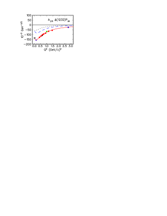
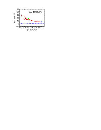
Figure 1: The $Q^{2}$ dependence of the $N\rightarrow\Delta$ helicity amplitudes. The solid and dashed curves are the results of the superglobal fit with MAID and the predictions of the hyperspherical constituent quark model. The dotted lines show the pion cloud contributions calculated with DMT. The data points at finite $Q^{2}$ are the results of our single-Q² fits, see Table 1 for references. At $Q^{2}=0$ for $A_{1/2}$ and $A_{3/2}$ the photon couplings from PDG are shown PDG02 .

4 Data analysis

The unitary isobar model MAID was used to analyze the world data base of pion photoproduction and recent differential cross section data on $p(e,e^{\prime}p)\pi^{0}$ from Mainz, Bates, Bonn and JLab. These data cover a $Q^{2}$ range from $0.1\cdots 4.0$ (GeV/c)² and an energy range $1.1<W<2.0$ GeV, see Table 1. In a first attempt we have fitted each data set at a constant $Q^{2}$ value separately. This is similar to a partial wave analysis of pion photoproduction and only requires additional longitudinal couplings for all the resonances. The $Q^{2}$ evolution of the background, Born terms and vector meson exchange, is described with a standard dipole form factor. In a second attempt we have introduced a $Q^{2}$ evolution of the transition form factors of the nucleon to $N^{*}$ and $\Delta$ resonances and have parameterized each of the transverse ($A_{1/2}$ and $A_{3/2}$) and longitudinal ($S_{1/2}$) helicity amplitudes. In a combined fit with all electroproduction data from the world data base of GWU/SAID SAID and the data of our single-$Q^{2}$ fit we obtained a $Q^{2}$ dependent solution (superglobal fit). In Fig. 1 we show our results for the $\Delta(1232)$ excitation. Our superglobal fit agrees very well with our single-$Q^{2}$ fits, except for the 2 lowest points of $S_{1/2}$ from our analysis of the Hall B data. Whether this is an indication for a different $Q^{2}$ dependence has still to be investigated. Generally, all our single-$Q^{2}$ points are shown with statistical errors from $\chi^{2}$ minimization only. A much bigger error has to be considered for model dependence.

We also compare our empirical analyses with the predictions of the hypercentral constituent quark. It turns out that the transverse amplitudes of the quark model are about half of the magnitudes and for the longitudinal amplitude $S_{1/2}(Q^{2})$ the quark model gives essentially zero. This is due to the fact that in the empirical analysis the resonance contribution is fully dressed by the pion cloud which is not the case in a constituent quark model. As depicted in Fig. 2 a fully dressed resonance contribution is renormalized on each vertex and in the propagator.

Figure 2: Resonances with dressed and bare electromagnetic vertices.

The baryonic states of the hCQM including hyperfine interaction can be considered as resonances dressed by hadronic interaction giving rise to the empirical masses. However, the electromagnetic vertex correction (third part of Fig. 2) is not included and has to be calculated separately. We have already started to do this and in a first attempt we have used the dynamical model DMT and extracted the pion loop contributions for the s- and p-waves. This estimate of the pion cloud vertex correction is shown as dotted lines in the figures. For the longitudinal Delta excitation the entire amplitude is practically given by the pion cloud contribution and only a negligible part arises from a bare Delta. The same is true for the electric amplitude which is given by the combination $A_{1/2}-A_{3/2}/\sqrt{3}$. This calculation also explains why none of the constituent quark models was ever able to give the empirical strength of the M1 excitation (or the transition moment $\mu_{N\Delta}$) of the $\Delta(1232)$. While in a simple $SU(2)$ calculation the transition moment is lower by about $30\%$ in more refined calculations it can be as low as only half of the empirical value. This is also the case here in our hCQM, even if it has more realistic wave functions.

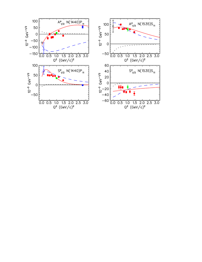
Figure 3: The $Q^{2}$ dependence of the transverse and longitudinal helicity amplitudes for the $P_{11}(1440)$ and the $S_{11}(1535)$ resonance excitation. The notation of the curves and the data is the same as in Fig. 1.

In Fig. 3 we show our results for the helicity amplitudes of the Roper resonance $P_{11}(1440)$ and the $S_{11}(1535)$. For these resonance amplitudes the pion cloud contributions are most important near the photon point and become already negligible around $Q^{2}=0.5$ GeV². The comparison between the hCQM and the empirical amplitudes is reasonably good, except for the $A_{1/2}$ amplitude of the Roper. This finding has to be further investigated both in the framework of the quark model and also in the empirical analysis. Certainly, for the Roper resonance the existing data is not very sensitive to this partial wave. Further experiments with double polarization could be very helpful to solve this problem.

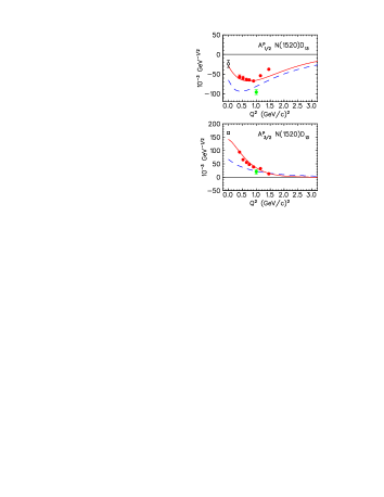
Figure 4: The $Q^{2}$ dependence of the transverse helicity amplitudes for the $D_{13}(1520)$ resonance excitation. The notation of the curves and the data is the same as in Fig. 1.

Finally, in Figs. 4 and 5 we show our results for the $D_{13}(1520)$ and the $F_{15}(1680)$ resonances. Here the largest discrepancies between our quark model calculations and the empirical analysis appear in the helicity $3/2$ amplitudes at small $Q^{2}$. So far, the dynamical model calculations have only been done for $s$- and $p$- waves, therefore we cannot give a pion cloud calculations for these partial waves. However, our findings encourages very strongly such extensions of the dynamical model. Furthermore we also have some empirical results for the partial waves that are not shown here, but most of them come out of the fit with rather large errors bars in the single-$Q^{2}$ analysis. This gives us less confidence also for our superglobal fit. The reason for it is mainly that we have fewer data points to analyze at higher energies.

5 Conclusions

Using the world data base of pion photo- and electroproduction and recent data from Mainz, Bonn, Bates and JLab we have made a first attempt to extract all longitudinal and transverse helicity amplitudes of nucleon resonance excitation for four star resonances below $W=2$ GeV. For this purpose we have extended our unitary isobar model MAID and have parametrized the $Q^{2}$ dependence of the transition amplitudes. Comparisons between single-$Q^{2}$ fits and a $Q^{2}$ dependent superglobal fit give us confidence in the determination of the Delta amplitudes. We can also reasonably well determine the amplitudes of the $P_{11}(1440),S_{11}(1535),D_{13}(1520)$ and the $F_{15}(1680)$, even though the model uncertainty of these amplitudes can be as large as 50% for the longitudinal amplitudes of the $D_{13}$ and $F_{15}$.

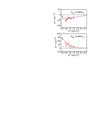
Figure 5: The $Q^{2}$ dependence of the transverse helicity amplitudes for the $F_{15}(1680)$ resonance excitation. The notation of the curves and the data is the same as in Fig. 1.

For other resonances the situation is even worse. However, this only reflects the fact that precise data in a large kinematical range are absolutely necessary. In some cases double polarization experiments are very helpful as has already been shown in pion photoproduction. Furthermore, without charged pion electroproduction, some ambiguities between partial waves that differ only in isospin as $S_{11}$ and $S_{31}$ cannot be resolved without additional assumptions. Finally, all results discussed here are only for the proton target. We have also started an analysis for the neutron, where much less data are available from the world data base and no new data has been analyzed in recent years. Since we can very well rely on isospin symmetry, only the electromagnetic couplings of the neutron resonances with isospin $1/2$ have to be determined. We have found such a solution for the neutron and will implement it in the next version of MAID (MAID2003). It will be a challenge for the experiment to investigate also the neutron resonances in the near future.

6 Acknowledgements

We wish to thank T. Bantes, G. Laveissiere and C. Smith for their contribution on the experimental data. This work was supported in part by the Deutsche Forschungsgemeinschaft (SFB443).

References

- (1) G. Höhler et al., Handbook of Pion-Nucleon Scattering, Physics Data 12-1 (Karlsruhe, 1979).
- (2) K. Hagiwara et al. (Particle Data Group), Phys. Rev. D 66 (2002) 010001.
- (3) S.J. Dong, T. Draper, I. Horvath, F.X. Lee, K.F. Liu, N. Mathur and J.B. Zhang, hep-ph/0306199.
- (4) For an overview and further references see S. Boffi, C. Giusti, F.D. Pacatiand M. Radici, Electromagnetic Response of Atomic Nuclei, Clarendon Press, Oxford, 1996, p. 114ff.
- (5) R. Beck et al., Phys. Rev. C 61 (2000) 035204.
- (6) S. Kamalov, S.N. Yang, D. Drechsel, O. Hanstein, L. Tiator, Phys. Rev. C 64 (2001) 032201; http://www.kph.uni-mainz.de/MAID/DMT/.
- (7) D. Drechsel, O. Hanstein, S.S. Kamalov and L. Tiator, Nucl. Phys. A645 (1999) 145; http://www.kph.uni-mainz.de/MAID/.
- (8) S.N. Yang, J. Phys. G 11 (1985) L205.
- (9) S.S. Kamalov and S.N. Yang, Phys. Rev. Lett. 83 (1999) 4494.
- (10) R.A. Arndt, I.I. Strakovsky and R.L. Workman, Phys. Rev. C 56 (1997) 577.
- (11) M. Ferraris, M.M. Giannini, M. Pizzo, E. Santopinto and L. Tiator, Phys. Lett. B364, 231 (1995).
- (12) Gunnar S. Bali, Phys. Rep. 343, 1 (2001).
- (13) N. Isgur and G. Karl, Phys. Rev. D18, 4187 (1978); D19, 2653 (1979); D20, 1191 (1979); S. Godfrey and N. Isgur, Phys. Rev. D32, 189 (1985);
- (14) M.M. Giannini, E. Santopinto, A. Vassallo, Eur.Phys.J. A12, 447 (2001); Nucl.Phys.A699,308 (2002).
- (15) M. Aiello, M. Ferraris, M.M. Giannini, M. Pizzo and E. Santopinto, Phys. Lett. B387, 215 (1996).
- (16) M. Aiello, M. M. Giannini, E. Santopinto, J. Phys. G: Nucl. Part. Phys. 24, 753 (1998)
- (17) M. De Sanctis, E. Santopinto, M.M. Giannini, Eur. Phys. J. A1, 187 (1998).
- (18) M. De Sanctis, M.M. Giannini, L. Repetto, E. Santopinto, Phys. Rev. C62,025208 (2000).
- (19) R.A. Arndt, W.J. Briscoe, I.I. Strakovsky and R.L. Workman, http://gwdac.phys.gwu.edu/.
- (20) Th. Pospischil et al., Phys. Rev. Lett. 86 (2001) 2959.
- (21) C. Mertz et al., Phys. Rev. Lett. 86 (2001) 2963.
- (22) T. Bantes and R. Gothe, private communication.
- (23) G. Laveissiere et al., Proc. of NSTAR2001, Mainz, World Scientific 2001, p 271 and private communications.
- (24) K. Joo et al., Phys. Rev. Lett. 88 (2002) 122001-1.
- (25) V.V. Frolov et al., Phys. Rev. Lett. 82 (1999) 45.