Meson loop effects on the pion electromagnetic form factor
Abstract
In this work we calculate the meson loop effects on the pion electromagnetic form factor and perform a comparison with experimental data. We show that, even though the meson cloud is not the only nonperturbative process to be considered, its contribution is significant.
I Introduction
The pion electromagnetic form factor has been under intense investigation both experimentally and theoretically. Yet there are still some open questions. Perhaps the most intriguing one is: why experimental data in the region of are still so far away from the perturbative QCD (pQCD) expectation? Or equivalently, what is the nonpertubative dynamics responsible for this behavior? Since long ago it has been suspected that the transition to the pQCD regime might happen at intermediate values of () [1, 2, 3]. However, the data from Jefferson Laboratory (JLAB) [4] are not only far from the pQCD prediction but follow a different trend.
Lattice calculations, in spite of their rapid progress [5], are not yet in position to answer the questions above. In order to elucidate the subject many models have been advanced. A variety of constituent quark models has been considered [6, 7, 8, 9]. Most of them are based on solutions of the light front Bethe-Salpeter equation with some approximations . In general, they achieve good agreement with data. Along a different line, the instanton model developed in Ref. [10] was able to give a reasonable description of data in the region . In a similar approach the same conclusion was found in [11].
In this work we consider the contribution of the meson cloud around the pion to its eletromagnetic form factor. This nonperturbative, hadronic effect was shown to play an important role in the electromagnetic form factor of the nucleon [12, 13, 14, 15, 16]. Recently the effect of the pion cloud was considered in the study of the pion form factor in the timelike region [17]. The meson, provenient from the photon was converted into a virtual pion loop. Using the same approach and the same kind of vertices, we compute mesonic loop contribution to the pion form factor in the spacelike region.
The idea of describing a pion with cloud states has already been used in [18] and also by us previously in [19], where we have studied asymmetry produced in collisions. In that work we could see that the inclusion of the meson cloud leads to a good agreement with experimental data.
In the next section we will review a few formulas used in the form factor calculations and define the dominant processes. In section III we discuss the inputs for the calculations and the numerical results. In section IV we present some concluding remarks.
II Loops and the pion form factor
The pion electromagnetic form factor is defined by:
| (1) |
where is the electromagnetic current. As in the case of the nucleon, we can represent the pion as a “bare pion” which can fluctuate into virtual Fock states composed by a pseudo-scalar (P) meson and a vector (V) meson, such as:
| (2) |
Thus, we can understand the photon-pion interaction as being an interaction between the photon and the constituents of the cloud. Usually the meson loop contributions are supposed to be dominant at low values of , where the incoming photon does not yet resolve quarks inside the pion. At higher values of , quark pointlike structures should become visible and a description of the problem in terms of hadronic degrees of freedom should loose validity.
However, due to the present difficulty in understanding the intermediate data, we consider the meson cloud contributions up to .
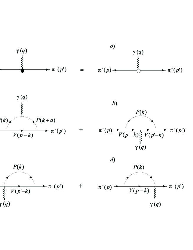
In Fig. 1 we show the first terms generated by the expansion (2): first the interaction between the photon and the bare pion (1o) and then the interaction between the photon and states composed by a pseudoscalar meson and a vector meson (1a-d). The full and open circles represent the dressed form factor and the form factor of the bare pion, respectively.
Before presenting the calculations some remarks are in order. Quite generally, the structure, or size, of any hadron depends on its quark content, on its meson cloud and on its off-shellness. We want to isolate and compute the strength of the meson cloud contribution. Looking at Fig. 1 and comparing the pion in the l.h.s. of the equality with the pion in a) we realize that the first one is on-shell, whereas the second one is off-shell. Therefore they are not exactly the same object and do not have the same structure. Moreover the pion in Fig. 1a) is a bare pion whereas the pion on the l.h.s. of the equality is composed by a bare pion plus the sum over all cloud corrections. With these considerations we want to emphasize that the l.h.s. pion and the pion within the loop are not the same.
In order to calculate de diagrams of Fig. 1 we start from the interaction Lagrangian given by:
| (3) |
where P and V denote a pseudoscalar and a vector meson respectively. From we derive the Feynman rules with which we write the vertex function associated with diagram (a) of Fig. 1:
| (4) |
and with diagram (b):
| (5) | |||
| (6) |
where and are the charges of the pseudoscalar and vector mesons, and and are their propagators. They are given by:
and
where and are the masses of the pseudoscalar and vector mesons respectively.
In order to account in some way for the finite extent of the mesons appearing in the loops of Fig. 1, we have included form factors in the hadronic vertices. For simplicity we have chosen a monopole form:
| (7) |
where is the cut-off parameter. Although there is no rigorous justification for this choice, form factors of this type have been used for example in Ref. [17]. These form factors render all the following loop integrals finite.
In the presence of the electromagnetic field the nonlocal mesonic interaction of Eqs. (3) and (7) gives rise to vertex currents. In order to maintain gauge invariance we introduce the photon field by minimal substitution of the momentum variable in the form factors. This procedure generates nonlocal seagull vertices [20]. They are:
| (8) |
for diagram (c) and
| (9) |
for diagram (d). Using the expressions above to write the functions for diagrams (c) and (d) we find respectively:
| (10) |
and
| (11) |
Due to the presence of the derivative in Eq. (3), the minimal substitution also generates current-vertex couplings even if the mesonic form factors are not present. They are:
| (12) |
for diagram (c) and
| (13) |
for diagram (d). Repeating the procedure used above, we write the functions for diagrams (c) and (d) using (12) and (13):
| (14) |
and
| (15) |
In order to obtain the total vertex function , we add (4), (6), (10), (11), (14) and (15) to find:
| (16) |
The pion electromagnetic form factor is associated with the term:
| (17) |
Since in the case of the pion it has not been discussed before we shall, in the remainder of this section, briefly show that the inclusion of the terms (10), (11), (14) and (15) is crucial for the fullfilment of the Ward-Takahashi (W-T) identity. The W-T identity reads:
| (18) |
where
| (19) |
For diagram (a) we have:
| (20) |
and for diagram (b):
| (21) |
For the seagull coupling of diagrams (c) and (d):
| (22) | |||
| (23) |
and for the vertex coupling of diagrams (c) and (d):
| (24) | |||
| (25) |
Due to charge conservation, , and thus we have:
| (29) |
As it can be seen from the last factor in expression (4), we are using a pointlike coupling in the virtual pion - photon - virtual pion (Fig. 1a). Since this pion has already some structure, we might introduce a form factor in this coupling, given by its quark structure (already present in the bare pion). However, we are interested only in the meson cloud and not in modelling the bare pion. The most simple and consistent procedure is to take, as we did, a pointlike coupling and keep in mind that this will maximize the contribution of the cloud, since any possible form factor would be a decreasing function of , with maximum value equal to one (at ). In this way we are computing the upper value for the cloud contribution.
Being restricted to the cloud contribution and making no attempt to accurately describe the data, we have only one parameter (the cut-off Lambda in our meson-meson-meson form factors), which is constrained by other types of phenomenological analyses. We have thus little freedom and therefore some predictive power.
III Numerical results and discussion
In order to compute the form factor (17), it is necessary to know the value of the relevant masses, coupling constants and cut-off parameters . The , coupling constants have been measured experimentally [21]. As the masses are all known, only the cut-off values remain as free parameters. So far there is no systematic study which indicates the most appropriate cut-off value for the vertices involving pion-meson-meson fluctuations. Since we are using a monopole parametrization for these vertices, we have chosen cut-off values close to the corresponding vector meson masses. In Table I we present all the values used in these calculations.
![[Uncaptioned image]](/html/nucl-th/0310039/assets/x2.png)
Table I: Values of coupling constants and cut-off used in the vertex functions.
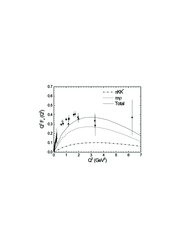
In order to explicitly show the relative strength of each cloud state, we show in Fig. 2 an example of result obtained with (17) and a cut-off fixed to GeV for the sum of states (dashed line), the sum of states (dot-dashed line), and the sum of all of them (solid line). We include the experimental data from the collaboration [4], from Amendolia et al. [22], from DESY [23] and from Bebeck et al. [24]. As it can be seen, all the curves rise , reach a maximum and then drop continuously. The heigth and relative strength of each contribution is controlled by the masses, couplings and cut-off values.

In Fig. 3 we show the contribution of the sum of all the meson cloud states to the pion form factor for several cut-off choices. We can observe a strong cut-off dependence. Nevertheless it is possible to conclude that the cloud contribution is significant specially in the region . Compared to the case of the nucleon electromagnetic form factor [13] the meson cloud plays here a less important role.
For each choice of cut-off parameter in Fig. 3 we have calculated the corresponding mean square radius , according to the usual definition:
| (30) |
The results are presented in Table II.
![[Uncaptioned image]](/html/nucl-th/0310039/assets/x5.png)
Table II: The mean square radius for different cut-off values.
We can see that, whatever the cut-off choice is, the mean square radius is much smaller than the experimental value [22].
In Fig. 4 we plot the form factor without multiplying it by to show in detail the behavior of our curves at low values of .
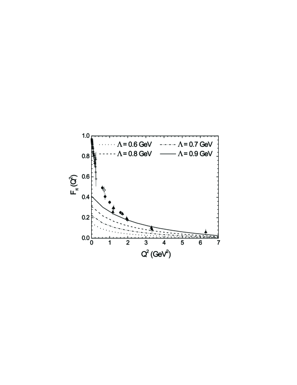
The results in Figs. 3 and 4 indicate that the cloud contribution underestimates the data in the low region. At higher values of ( ), it starts to be closer to data. In the asymptotic limit the cloud contribution vanishes. Since we did not make any model for the bare pion, its influence on the form factor is a priori unknown. Looking at the results presented in Fig. 4, we can just observe that there is room for a significant bare pion contribution.
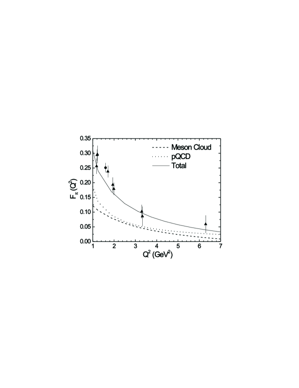
Perturbative QCD predicts that in the high region the form factor should be much smaller than the actually measured data. The cloud component is then a candidate to be the nonperturbative complement to pQCD. In order to further investigate the relation bewteen the cloud and pQCD, we make now the simplifying assumption that in the asymptotic region the bare pion contribution is simply given by pQCD. The physical picture becomes quite simple: a highly virtual photon probes a pion which is either the ”core” or the cloud. In the first case the photon interacts with the quarks in the perturbative regime. In the second case, the photon interacts with a hadron of the cloud. In practice, the above assumption means adding to the cloud a contribution which is known and given by [10]:
| (31) |
where and . This expression is plotted in Fig. 5 with a dotted line and it is added to the previously computed cloud contribution for , represented by the dashed line. We can see that the sum of the two contributions (solid line) gives a good description of data in the region . In Fig. 5 we can clearly observe how, at large , the cloud contribution dies out while pQCD takes over. Although our results are not definitive, they strongly suggest that a hard cut-off ( ) is hard to accomodate, if one is bound to reproduce data leaving room for a sizeable bare pion (pQCD) component.
IV Concluding remarks
Meson loop effects are a necessary consequence of quantum field theory and must be considered in the analysis of any hadronic observable. We have performed a straightforward extension of standard one loop calculations to the pion form factor. The main goal was to estimate the magnitude of the meson cloud contribution to . It turned out to be less important than the meson cloud contribution to the nucleon form factor [13]. This is not unexpected since, because of the masses and corresponding virtualities, it is much easier for a proton to be in a neutron-pion state than it is for a pion to fluctuate into a pion-rho state.
The size of the cloud contribution must also be cross checked with that in deep inelastic scattering (DIS), as discussed in [18]. In Fig. 4 we can see that the size of the cloud contribution depends on the value of . At around zero it represents something between and of the total form factor. This fraction is consistent with other estimates [18], coming from DIS and high energy inclusive hadron-hadron collisions. In [18], a smaller percentage was found for the cloud contribution. This discrepancy is probably due to the different methods used to extract the strength of the cloud states and also because different experimental data were considered. As increases, the relative contribution of the cloud increases, but this region it is difficult to draw firm conclusions because the model gradually runs out of its domain of applicability and also, as stated above, our procedure gives an upper bound for the cloud contribution.
The calculation presented here is model dependent in the sense that we have truncated a series (of cloud states) and replaced the effects of the higher order terms by form factors, which also account for the quark substructure of mesons. Since we have used the same type of form factor and the same cut-off for all vertices we have only one parameter, , which was already constrained by our previous knowledge of hadronic interactions. It should lie in the interval . Our results confirm this expectation and also suggest that the cut-off should rather be in the range GeV if we believe that that the cloud contribution is of the order of or less.
The fact that meson loops can not
describe data in the low
region, regardless of cut-off choice, confirms that another
dynamics is missing in this
region, as, for example, the interaction of the photon with
constituent quarks.
Acknowledgements This work was partially supported by CAPES, CNPq and FAPESP under contract 00/04422-7.
REFERENCES
- [1] G.P. Lepage and S.J. Brodsky, Phys. Rev. D22, 2157 (1980).
- [2] R. Jakob and P. Kroll, Phys. Lett. B315, 463 (1993).
- [3] O.C. Jacob and L.S. Kisslinger, Phys. Lett. B243, 323 (1990).
- [4] J. Volmer et al. Phys. Rev. Lett. 86, 1713 (2001).
- [5] J. van der Heide, M. Lutterot, J.H. Koch and E. Laermann, Phys. Lett. B566, 131 (2003). and references therein.
- [6] F. Cardarelli, I. Grach, I. Narodetskii, E. Pace, G. Salmé, S. Simula, Phys. Rev. D53, 6682 (1996); F. Cardarelli, E. Pace, G. Salme’, S. Simula, Phys. Lett. B357, 267 (1995).
- [7] P. Maris, nucl-th/0209048; P. Maris, P.C. Tandy, Phys. Rev. C61, 045202 (2000).
- [8] J.P.B.C. de Melo, T. Frederico, E. Pace, G. Salmé, Nucl. Phys. A707, 399 (2002); J.P.B.C. de Melo, H.W.L. Naus and T. Frederico, Phys. Rev. C59, 2278 (1999).
- [9] H.-M. Choi, L.S. Kisslinger and C.-R. Ji, Nucl. Phys. Proc. Suppl. 108, 310 (2002); L.S. Kisslinger, H.-M. Choi and C.-R. Ji, Phys. Rev. D63, 113005 (2001) and references therein.
- [10] P. Faccioli, A. Schwenk and E.V. Shuryak, Phys. Rev. D67, 113009 (2003).
- [11] H. Forkel and M. Nielsen, Phys. Lett. B345, 55 (1997).
- [12] J. Friedrich and Th. Walcher, Eur. Phys. J. A17, 607 (2003).
- [13] G. A. Miller, nucl-th/0206027.
- [14] A.Yu. Korchin, Eur. Phys. J. A11, 427 (2001).
- [15] D.H. Lu, S.N. Yang and A.W. Thomas, J. Phys. G26, L75 (2000).
- [16] H.C. Doenges, M. Schaefer and U. Mosel, Phys. Rev. C51, 950 (1995).
- [17] D. Melikhov, O. Nachtmann, T. Paulus, hep-ph/0209151.
- [18] A. Szczurek, H. Holtmann and J. Speth, Nucl. Phys. A605, 496 (1996); Nucl. Phys. A728, 182 (2003).
- [19] F. Carvalho, F. O. Durães, F. S. Navarra and M. Nielsen, Phys. Rev. Lett. 86, 5434 (2001); Phys. Rev. D60, 094015 (1999).
- [20] K. Ohta, Phys. Rev. D35, 785 (1987); L. L. Barz et al., Nucl. Phys. A640, 259 (1998); Braz. J. Phys. 27, 358 (1997); H. Forkel et al., Nucl. Phys. A680, 179 (2000).
- [21] see, for exeample, S. L. Zhu, Eur. Phys. J. A4, 277 (1999) and references therein.
- [22] S. R. Amendolia et al., Nucl. Phys. B277, 168 (1986).
- [23] P. Brauel et al., Z. Phys. C3, 101 (1979).
- [24] C. J. Bebeck et al., Phys. Rev. D17, 1693 (1978).