Nonequilibrium chiral dynamics by the time dependent variational approach
with squeezed states

Abstract

We investigate the inhomogeneous chiral dynamics of the O(4) linear sigma model in 1+1 dimensions using the time dependent variational approach in the space spanned by the squeezed states. We compare two cases, with and without the Gaussian approximation for the Green’s functions. We show that mode-mode correlation plays a decisive role in the out-of-equilibrium quantum dynamics of domain formation and squeezing of states.

The possibility of the formation of the disoriented chiral condensate (DCC) in high energy heavy ion collisions has been extensively studied with various methods. In classical approximation ref:classical01 ; ref:classical02 , it has been shown that the amplification of long wavelength modes of the pion fields takes place when the system starts with the nonequilibrium initial condition, quench initial condition ref:classical01 ; ref:classical02 . In addition to the amplification, spatial correlation of the fields has been also shown to grow.

Although the classical approximation is expected to work well in incorporating nonequilibrium aspects of the system when pion density is large, it is still desirable to include quantum effects. In fact, investigations in this direction have been also carried out extensively with the Hartree approximation, the large $N$ approximation, and so on boyanovski01 ; cooper01 . In most of the previous studies which include quantum effects, however, it has been assumed that the system is spatially homogeneous. Problems such as insufficient thermalization at late times and impossibility to describe domain structures have been recognized. It has not been conclusive whether there is a chance for the correlations to grow through nonequilibrium time evolution.

There are at least two ways for possible improvement. One is to include higher order quantum corrections and the other is to accommodate spatial inhomogeneity. We will pursue the latter in this paper. Recently, the dynamics of spatially inhomogeneous system has been studied by several groups quantum mechanically berges ; cooper02 ; smit ; bettencourt and it has been shown that the thermalization of the quantum fields can occur. In these works, the Gaussian approximation, in which the Green’s functions are assumed to be diagonal in momentum space, has been adopted because of computational reasons. Physically, it corresponds to ignoring correlations between modes with different momenta, and under the approximation different modes can interact only through the mean fields. However, it is possible that the direct coupling of modes through the off-diagonal correlations is important for the time evolution of the system when the system does not possess translational invariance. To see if such an effect is substantial, we study the dynamics of chiral phase transition in spatially inhomogeneous systems with off-diagonal components of the Green’s function in momentum space fully taken into account.

In this paper, we take the O(4) linear sigma model as a low energy effective theory of QCD and apply the method of the time dependent variational approach (TDVA) with squeezed states. This method was originally developed by Jackiw and Kerman as an approximation in the functional Schrödinger approach JK and later it was shown to be equivalent to TDVA with squeezed states by Tsue and Fujiwara TF .

In this approach, the trial state is a squeezed state

$$|\Phi(t)\rangle = \prod_{a}|\Phi_{a}(t)\rangle,$$

$$|\Phi_{a}(t)\rangle = \exp\bigl{[}S_{a}(t)\bigr{]}\cdot N_{a}(t)\cdot\exp\bigl{[}T_{a}(t)\bigr{]}|0\rangle,$$

$$S_{a}(t) = i\int d\vec{x}\bigl{[}C_{a}(\vec{x},t){\phi_{a}}(\vec{x})-D_{a}(\vec{x},t){\pi_{a}}(\vec{x})\bigr{]},$$

$$T_{a}(t) = \int d\vec{x}d\vec{y}\phi_{a}(\vec{x})\Bigl{[}-\frac{1}{4}\bigl{[}G_{a}^{-1}(\vec{x},\vec{y},t)$$ (1)

$$-G_{a}^{(0)-1}(\vec{x},\vec{y})\bigr{]}+i\Pi_{a}(\vec{x},\vec{y},t)\Bigr{]}\phi_{a}(\vec{y}),$$

where $a$ runs from 0 to 3. $a=0$ is for the sigma field and $a=1-3$ are for the pion fields. $|0\rangle$ is the reference vacuum and $G_{a}^{(0)}(\vec{x},\vec{y})=\langle 0|\phi_{a}(\vec{x})\phi_{a}(\vec{y})|0\rangle$. $\phi_{a}(\vec{x})$ and $\pi_{a}(\vec{x})$ are the field operator and conjugate field operator for the field $a$, respectively. $C_{a}(\vec{x},t)$, $D_{a}(\vec{x},t)$, $G_{a}(\vec{x},\vec{y},t)$, and $\Pi_{a}(\vec{x},\vec{y},t)$ are the mean field variables for $\phi_{a}$ field at $\vec{x}$ and $t$, the canonical conjugate variable for the mean field, the quantum correlation for $\vec{x}\neq\vec{y}$ (fluctuation around the mean field for $\vec{x}=\vec{y}$), and the canonical conjugate variable for $G_{a}(\vec{x},\vec{y},t)$, respectively, and all of them are real functions. $N_{a}(t)$ is a normalization constant. $T(t)$ is an operator that describes the squeezing, and if $T_{a}(t)$ is set to 0, $|\Phi_{a}(t)\rangle$ is reduced to a coherent state with the expectation values of $\phi(\vec{x},t)$ and $\pi(\vec{x},t)$ given by $C_{a}(\vec{x},t)$ and $D_{a}(\vec{x},t)$, respectively.

The Hamiltonian $H$ of the O(4) linear sigma model is given by

$$H = \int d\vec{x}\sum_{a=0}^{3}\biggl{\{}\frac{1}{2}\pi_{a}(\vec{x})^{2}+\frac{1}{2}\vec{\nabla}\phi_{a}(\vec{x})\cdot\vec{\nabla}\phi_{a}(\vec{x})$$ (2)

$$+\lambda\bigl{[}\phi_{a}(\vec{x})^{2}-v^{2}\bigr{]}^{2}-h\phi_{0}(\vec{x})\biggr{\}}.$$

As shown in Eq. (1), the trial state is specified by $C_{a}(\vec{x},t)$, $D_{a}(\vec{x},t)$, $G_{a}(\vec{x},\vec{y},t)$, and $\Pi_{a}(\vec{x},\vec{y},t)$. Their time evolution is determined through the time dependent variational principle:

$$\delta\int dt\langle\Phi(t)|i\frac{\partial}{\partial t}-H|\Phi(t)\rangle=0.$$ (3)

In this approach, correlation between different modes in momentum space arises through the scattering of quanta caused by the nonlinear coupling term in the model Hamiltonian even if there is initially no such correlation. This can be seen best from the following equations of motion in momentum space,

$$\ddot{C}_{a}(\vec{k},t) = -\vec{k}^{2}-\mathcal{M}_{a}^{(1)}(\vec{k},t),$$

$$\dot{G}_{a}(\vec{k},\vec{k}^{\prime},t) = 2\langle\vec{k}|\left[G_{a}(t)\Pi_{a}(t)+\Pi_{a}(t)G_{a}(t)\right]|\vec{k}^{\prime}\rangle,$$

$$\dot{\Pi}_{a}(\vec{k},\vec{k}^{\prime},t) = \mbox{$\frac{1}{8}$}\langle\vec{k}|G_{a}^{-1}(t)G_{a}^{-1}(t)|\vec{k}^{\prime}\rangle-2\langle\vec{k}|\Pi_{a}(t)\Pi_{a}(t)|\vec{k}^{\prime}\rangle$$

$$-\vec{k}^{2}\delta^{3}(\vec{k}-\vec{k}^{\prime})-\mbox{$\frac{1}{2}$}\mathcal{M}_{a}^{(2)}(\vec{k}-\vec{k}^{\prime},t),$$

$$\mathcal{M}_{a}^{(1)}(\vec{k},t) = \Bigl{[}-m^{2}+4\lambda C_{a}^{2}(\vec{k},t)+12\lambda G_{a}(\vec{k},\vec{k},t)$$

$$+4\lambda\sum_{b(\neq a)}\bigl{(}C_{b}^{2}(\vec{k},t)+G_{b}(\vec{k},\vec{k},t)\bigr{)}\Bigr{]}C_{a}(\vec{k},t)$$

$$-h\delta_{a0},$$

$$\mathcal{M}_{a}^{(2)}(\vec{k},t) = -m^{2}+12\lambda C_{a}^{2}(\vec{k},t)+12\lambda G_{a}(\vec{k},\vec{k},t)$$ (4)

$$+4\lambda\sum_{b(\neq a)}\left(C_{b}^{2}(\vec{k},t)+G_{b}(\vec{k},\vec{k},t)\right),$$

where $m^{2}=4\lambda v^{2}$, and $C_{a}(\vec{k},t)$, $G_{a}(\vec{k},\vec{k}^{\prime},t)$, and $\Pi_{a}(\vec{k},\vec{k}^{\prime},t)$ are the mean fields for the $\phi_{a}$ field with momentum $\vec{k}$, the correlation between modes with momenta $\vec{k}$ and $\vec{k}^{\prime}$ for $\vec{k}\neq\vec{k}^{\prime}$ (the quantum fluctuation around the mean field for $\vec{k}=\vec{k}^{\prime}$), the canonical conjugate variable for $G_{a}(\vec{k},\vec{k}^{\prime},t)$, respectively. In Eq. (4), we have used the notation,

$$\langle\vec{k}|H(t)I(t)|\vec{k}^{\prime}\rangle=\int\frac{d\vec{k}^{\prime\prime}}{(2\pi)^{3}}H(\vec{k},\vec{k}^{\prime\prime},t)I(\vec{k}^{\prime\prime},\vec{k}^{\prime},t).$$ (5)

In the Gaussian approximation, $G_{a}(\vec{k},\vec{k}^{\prime},t)$ and $\Pi_{a}(\vec{k},\vec{k}^{\prime},t)$ are set to zero for $\vec{k}\neq\vec{k}^{\prime}$ and correlations between different modes in momentum space are ignored. However, $\mathcal{M}^{(2)}(\vec{k}-\vec{k}^{\prime},t)$ in Eq. (4), which originates from the four-point interaction terms in the O(4) linear sigma model, couples modes with different momenta and correlations between them develop even if initially there exists no correlation among them.

In numerical calculation, we have assumed the one-dimensional spatial dependence for the mean fields and the Green’s functions for computational simplicity. In addition, we have imposed the periodic boundary condition for the mean fields and the Green’s functions. We have carried out calculation on a lattice with the lattice spacing $d=1.0$ fm and the total length $L=64$ fm, which leads to the momentum cutoff $\Lambda=1071$ MeV. The parameters $\lambda$, $v$, and $h_{0}$ are determined so that they give the pion mass $M_{\pi}=138$ MeV, the sigma meson mass $M_{\sigma}=500$ MeV, and the pion decay constant $f_{\pi}=93$ MeV in the vacuum following the prescription given in Ref. TKI , and we have obtained $\lambda=3.44$, $v=110$ MeV, and $h_{0}=(103~{}\rm{MeV})^{3}$ .

There are several scenarios for the DCC formation in high energy heavy ion collisions. Here we adopt the quench scenario. In this scenario, the chiral order parameters remain around the top of the Mexican hat potential after the rapid change of the effective potential from the chirally symmetric phase to the chirally broken phase. In order to take this situation into account, we have used the following initial condition; at each lattice point, the mean field variable for the chiral fields and their conjugate variables $C_{a}(\vec{x},0)$ and $D_{a}(\vec{x},0)$ are randomly distributed according to the Gaussian form with the following parameters AM ,

$$\langle C_{a}(\vec{x},0)\rangle = 0,$$

$$\langle C_{a}(\vec{x},0)^{2}\rangle-\langle C_{a}(\vec{x},0)\rangle^{2} = \delta^{2},$$

$$\langle D_{a}(\vec{x},0)\rangle = 0,$$

$$\langle D_{a}(\vec{x},0)^{2}\rangle-\langle D_{a}(\vec{x},0)\rangle^{2} = \frac{D}{d^{2}}\delta^{2},$$ (6)

where $D=1$ is the spatial dimension and $\delta$ is the Gaussian width. We shall use $\delta=0.19v$ in the following calculations. In relating the Gaussian widths of $C_{a}(\vec{x},0)$ and $D_{a}(\vec{x},0)$, we have taken advantage of the virial theorem AM .

As for the initial conditions for the quantum fluctuation and correlation, we have assumed that their values are those realized in the case where each state in momentum space were in a coherent state with a degenerate mass $m_{0}$ for the sigma meson and pions, namely,

$$G_{a}(\vec{x},\vec{y},0)=\int_{0}^{\Lambda}\frac{d\vec{k}}{(2\pi)^{3}}\frac{1}{2\omega_{k}}e^{i\vec{k}\cdot(\vec{x}-\vec{y})},$$

$$\Pi_{a}(\vec{x},\vec{y},0)=0,$$ (7)

where $\omega_{k}=\sqrt{m_{0}^{2}+\vec{k}^{2}}$. We adopt $m_{0}=200$ MeV. As shown above, the Green’s functions $G_{a}(\vec{x},\vec{y},0)$ and $\Pi_{a}(\vec{x},\vec{y},0)$ are initially diagonal in momentum space. The off-diagonal components appear in the course of the time evolution of the system due to the direct mode-mode coupling induced by $\mathcal{M}^{(2)}$ in Eq. (4).

We have carried out two sets of numerical calculations. In one case, we have taken into account all components of the two-point Green’s functions (case I), while in the other case only the diagonal components of the two-point Green’s functions (case II) were included in the calculation as in most of the preceding works.

In Fig. 1, we show the time evolution of the mean fields for the sigma and the third component of the pion fields ($\phi_{0}$ and $\phi_{3}$, respectively) obtained with the calculation including all components of the Green’s functions (case I). As a whole, the expectation value of the sigma field approaches a constant. On the other hand, that of the pion field oscillates around zero and shows a domain structure with long correlation length. This is the formation of DCC domains. It is observed that the domain structure continues to grow till as late as $t\sim 40$ fm.

In Fig. 2, we show the time evolution of the same mean fields obtained with the Gaussian approximation, i.e., without the off-diagonal components of the Green’s functions (case II). At the beginning, the behavior of the mean fields is similar to that in case I. However, after a few femtometers, there appears a clear difference between the two cases. In case II, short range fluctuation is dominant and no long length correlation is observed. No qualitative change in the behavior of the mean fields takes place in case II after a few femtometers. This tells us that the mode-mode correlation plays a decisive role in the formation of DCC domains.

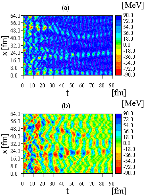
Figure 1: (Color online) Time evolution of the mean fields in case I. (a) and (b) are for the sigma field and the third component of the pion field, respectively.

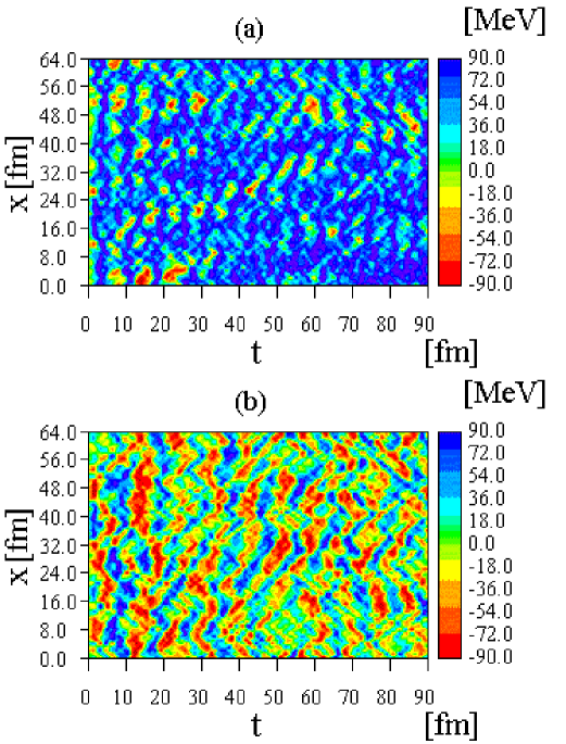
Figure 2: (Color online) Time evolution of mean fields in case II. (a) and (b) are for the sigma field and the third component of the pion field, respectively.

To examine the growth of spatial correlation of the pion fields more quantitatively, we define the following spatial correlation function $C(r,t)$,

$$C(r,t)=\frac{\int{\vec{\phi}}(\vec{x})\!\cdot\!{\vec{\phi}}(\vec{y})\delta(|\vec{x}-\vec{y}|-r)d\vec{x}d\vec{y}}{\int|{\vec{\phi}}(\vec{x})||{\vec{\phi}}(\vec{y})|\delta(|\vec{x}-\vec{y}|-r)d\vec{x}d\vec{y}},$$ (8)

where ${\vec{\phi}}(\vec{x})\!\cdot\!{\vec{\phi}}(\vec{y})=\sum_{i=1}^{3}{\phi_{i}}(\vec{x}){\phi_{i}}(\vec{y})$ and $|{\vec{\phi}}(\vec{x})|=\sqrt{\sum_{i=1}^{3}{\phi_{i}^{2}}(\vec{x})}$.

In Figs. 3(a) and 3(b), we show this spatial correlation function in cases I and II, respectively. The correlation functions are calculated by taking average over 10 events. Substantial generation of the correlation takes place after the typical time scale of the initial rolling down of the chiral fields, say, a few femtometers in case I, while the growth of the spatial correlation ends in case II by $t\sim 5$ fm. The domain formation of DCC shown in Fig. 1(b) and this growth of spatial correlation shown in Fig. 3(a) beyond the rolling down time scale may be related to the parametric resonance mrowczynski95 ; hiro-oka00 . We are currently investigating this possibility.

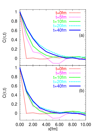
Figure 3: (Color online) The spatial correlations for the pion fields in case I (a) and case II (b).

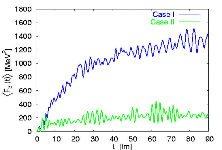
Figure 4: (Color online) The time evolution of the spatially averaged quantum fluctuation of the third component of the pion field, $\langle F_{3}(t)\rangle_{\rm space}$ for cases I and II.

Next we show the time evolution of the quantum fluctuation, which is represented by the same-point Green’s function $G_{a}(\vec{x},\vec{x},t)$. We define the spatially averaged fluctuation function $\langle F_{a}(t)\rangle_{{\rm space}}$ at time $t$ as

$$\langle F_{a}(t)\rangle_{{\rm space}}=\frac{1}{V}\int G_{a}(\vec{x},\vec{x},t)d{\vec{x}},$$ (9)

where $V$ is the volume of the system.

In Fig. 4, we compare the time evolution of the spatially averaged quantum fluctuation of the the third component of the pion field, $\langle F_{3}(t)\rangle_{{\rm space}}$ in the two cases. We observe remarkable increase of quantum fluctuation in case I, while only small amplification is seen in case II. This increase also lasts until about $t=40$ fm. The comparison between case I and case II tells us that the off-diagonal correlations take an important role also for the enhancement of the quantum fluctuation. We have in fact found the growth of off-diagonal components of the Green’s functions in momentum space. Note that this phenomenon cannot be described unless the off-diagonal correlation is introduced. This has an important meaning also for the identical particle correlation in high energy heavy ion collisions. Usually it is assumed that identical particles with different momenta are emitted independently. However, if there is quantum correlation between two different modes, this assumption becomes invalid, and it will be necessary to reformulate the theory for the identical particle correlation.

In summary, we have studied the inhomogeneous chiral dynamics of the O(4) linear sigma model in 1+1 dimensions using TDVA with squeezed states. We have compared two cases. One is a general case in which both the mean fields and the Green’s functions are inhomogeneous, and the other is a case with the Gaussian approximation, where translational invariance is imposed on the Green’s functions. We have shown for the first time that the large correlated domains can be realized in the quench scenario with quantum mechanical treatment. More specifically, we have shown that the large amplification of quantum fluctuation and large domain structure emerge when all components of the Green’s functions are retained, while only small quantum fluctuation and small and noisy domain structure are seen in the case with the Gaussian approximation. The dynamics in $1+2$ and $1+3$ dimensional cases is of great interest and indispensable for the understanding of the DCC formation in ultrarelativistic heavy ion collisions. We expect more enhanced domain growth in $1+2$ and $1+3$ dimensional cases because of the existence of more mode-mode correlations in such cases. We plan to confirm it by actual numerical calculation.

N.I. thanks the nuclear theory group at Kyoto University for encouragement. M.A. is partially supported by the Grants-in-Aid of the Japanese Ministry of Education, Science and Culture, Grants Nos. 14540255. Y.T. is partially supported by the Grants-in-Aid of the Japanese Ministry of Education, Science and Culture, Grants No. 13740159 and 15740156. Numerical calculation was carried out at Yukawa Institute for Theoretical Physics at Kyoto University and Tohoku-Gakuin University. We thank T. Otofuji for making it possible to use the computing facility at Tohoku-Gakuin University.

References

- (1) K. Rajagopal and F. Wilczek, Nucl. Phys. B404, 577 (1993).
- (2) M. Asakawa, Z. Huang, and X.-N. Wang, Phys. Rev. Lett. 74, 3126 (1995).
- (3) D. Boyanovsky, H. J. de Vega, and R. Holman, Phys. Rev. D 49, 2769 (1994); D. Boyanovsky, H. J. de Vega, R. Holman, D. S. Lee, and A. Singh, ibid. 51, 4419 (1995); D. Boyanovsky, H. J. de Vega, R. Holman, and J. Salgado, ibid. 59, 125009 (1999).
- (4) F. Cooper, S. Habib, Y. Kluger, E. Mottola, J. P. Paz, and P. R. Anderson, Phys. Rev. D 50, 2848 (1994); F. Cooper, Y. Kluger, E. Mottola, and J. P. Paz, ibid. 51, 2377 (1995).
- (5) J. Berges, Nucl. Phys. A699, 847 (2002); G. Aarts, D. Ahrensmeier, R. Baier, J. Berges, and J. Serreau, Phys. Rev. D 66, 045008 (2002).
- (6) F. Cooper, J. F. Dawson, and B. Mihaila, Phys. Rev. D 67, 056003 (2003).
- (7) M. Salle, J. Smit, and J. C. Vink, Phys. Rev. D 64, 025016 (2001); M. Salle, J. Smit, and J. C. Vink Nucl. Phys. B625, 495 (2002); G. Aarts and J. Smit, Phys. Rev. D 61, 025002 (2001).
- (8) L. M. A. Bettencourt, K. Pao, and J. G. Sanderson, Phys. Rev. D 65, 025015 (2002).
- (9) R. Jackiw and A. Kerman, Phys. Lett. A71, 158 (1979).
- (10) Y. Tsue and Y. Fujiwara, Prog. Theor. Phys. 86, 443 (1991); ibid. 86, 469 (1991).
- (11) Y. Tsue, A. Koike, and N. Ikezi, Prog. Theor. Phys. 106, 469 (2001) 807.
- (12) M. Asakawa, H. Minakata, and B.Müller, Phys. Rev. D 58, 094011 (1998).
- (13) S. Mrówczyński and B. Müller, Phys. Lett. B 363, 1 (1995).
- (14) H. Hiro-Oka and H. Minakata, Phys. Rev. C 61, 044903 (2000).