Strangeness production via electromagnetic probes: 40 years later

Abstract

A brief review of the associated strangeness electromagnetic production is presented. Very recent $K^{+}\Lambda$ photoproduction data on the proton from threshold up to $E_{\gamma}^{lab}$ = 2.6 GeV are interpreted within a chiral constituent quark formalism, which embodies all known nucleonic and hyperonic resonances. The preliminary results of this work are reported here.

1 Introduction

This conference witnessed the advent of thousands of data points from JLab/CLAS[1] and ELSA/SAPHIR[2] on the $K^{+}\Lambda$ and $K^{+}\Sigma^{\circ}$ photoproduction on the proton. Moreover, the recent data with polarized photon beam from Spring-8/LEPS[3] and with electrons from JLab[4] announce the start of a new era in this field, ringing the moment of the truth for phenomenologists!

Actually, this journey started some 40 years ago (see e.g. Ref.[5]), with the pionner and significant work performed by Thom[6]. The data which are now becoming available, were anticipated some 20 years ago and gave a new momentum to the phenomenological investigations[5, 7]. Those studies, based on the Feynman diagrammatic technique, included s-,u-, and t-channel contributions, and produced models differing mainly in their content of baryon resonances. Later, more sophistications were introduced[8, 9, 10, 11, 12, 13], the most significant ones being:

i) Introduction of spin- 3/2 and 5/2 nucleonic[9, 12] and spin-3/2 hyperonic resonances[10]. This latter would not have been possible without the incorporation[10] of the so-called off-shell effects inherent to the fermions with spin $\geq 3/2$, which of course also applies to the relevant nucleon resonances.

ii) Introduction of hadronic form factors at strong vertices and preserving the gauge invariance of the amplitudes[14].

The well known main difficulty in the kaon production, compared to the $\pi$ and $\eta$ cases, is that the reaction mechanism here is not dominated by a small number of resonances. This fact implies that we need to embody in the model contributions from a large number of resonances, the known ones being shown in Table I. Given that, according to the spin of the resonances, one needs 1 to 5 free parameters per resonance; it is obvious that a meaningful study of the resonance content of the underlying reaction mechanism is excluded within such approaches.

Table I. Baryon resonances[15] with mass $M_{N^{*}}\leq$ 2.5 GeV. Notations are $L_{2I~{}2J}(mass)$ and $L_{I~{}2J}(mass)$ for $N^{*}$ and $Y^{*}$, respectively.

Baryon	Three & four star resonances	One & two star resonances
	$S_{11}(1535)$, $S_{11}(1650)$,	$S_{11}(2090)$,
	$P_{11}(1440)$, $P_{11}(1710)$, $P_{13}(1720)$,	$P_{11}(2100)$, $P_{13}(1900)$,
$N^{*}$	$D_{13}(1520)$, $D_{13}(1700)$, $D_{15}(1675)$,	$D_{13}(2080)$, $D_{15}(2200)$,
	$F_{15}(1680)$,	$F_{15}(2000)$, $F_{17}(1990)$,
	$G_{17}(2190)$, $G_{19}(2250)$,
	$H_{19}(2220)$,
	$S_{01}(1405)$, $S_{01}(1670)$, $S_{01}(1800)$,
	$P_{01}(1600)$, $P_{01}(1810)$, $P_{03}(1890)$,
$\Lambda^{*}$	$D_{03}(1520)$, $D_{03}(1690)$, $D_{05}(1830)$,	$D_{03}(2325)$,
	$F_{05}(1820)$, $F_{05}(2110)$,	$F_{07}(2020)$,
	$G_{07}(2100)$,
	$H_{09}(2350)$,
	$S_{11}(1750)$,	$S_{11}(1620)$, $S_{11}(2000)$,
	$P_{11}(1660)$, $P_{11}(1880)$, $P_{13}(1385)$,	$P_{11}(1770)$, $P_{11}(1880)$,
$\Sigma^{*}$		$P_{13}(1840)$, $P_{13}(2080)$,
	$D_{13}(1670)$, $D_{13}(1940)$, $D_{15}(1775)$,	$D_{13}(1580)$,
	$F_{15}(1915)$, $F_{17}(2030)$.	$F_{15}(2070)$,
		$G_{17}(2100)$.

However, isobaric models provide us with useful tools, if other more appropriate formalisms allow us to single out the most relevant resonances in the reaction mechanism and determine their couplings in order to significantly reduce the number of free parameters. Such an opportunity is offered to us by a chiral constituent quark approach, as discussed in the next Section. Nevertheless, this latter being a non-relativistic formalism, can not be applied to the electroproduction processes, other than at low $Q^{2}$ kinematic region. So, a possible scenario could be to pin down the reaction mechanism in the photoproduction using the constituent quark formalism, then pick up the most relevant resonances and their couplings extracted via the quark model and embody them in the Feynman diagrammatic approach to study the electroproduction reactions. The capability of Feynman diagrammatic technique to provide the elementary operators and be used as input into the strangeness production on nuclei has already been proven[16]. Finally, the advent of realistic elementary operators in line with the above procedure implies coupled-channel treatments[17, 18].

In the following Sections, we will focus on the very recent $\gamma p\rightarrow K^{+}\Lambda$ data[1, 2] and study them via a chiral constituent quark approach based on the broken $SU(6)\otimes O(3)$ symmetry.

2 Theoretical Frame

The starting point of the meson photoproduction in the chiral quark model is the low energy QCD Lagrangian[19]

$${\mathcal{L}}={\bar{\psi}}\left[\gamma_{\mu}(i\partial^{\mu}+V^{\mu}+\gamma_{5}A^{\mu})-m\right]\psi+\dots$$ (1)

where $\psi$ is the quark field in the $SU(3)$ symmetry, $V^{\mu}=(\xi^{\dagger}\partial_{\mu}\xi+\xi\partial_{\mu}\xi^{\dagger})/2$ and $A^{\mu}=i(\xi^{\dagger}\partial_{\mu}\xi-\xi\partial_{\mu}\xi^{\dagger})/2$ are the vector and axial currents, respectively, with $\xi=e^{i\Pi f}$. $f$ is a decay constant and the field $\Pi$ is a $3\otimes 3$ matrix,

$$\Pi=\left|\begin{array}[]{ccc}\frac{1}{\sqrt{2}}\pi^{\circ}+\frac{1}{\sqrt{6}}\eta&\pi^{+}&K^{+}\\ \pi^{-}&-\frac{1}{\sqrt{2}}\pi^{\circ}+\frac{1}{\sqrt{6}}\eta&K^{\circ}\\ K^{-}&\bar{K}^{\circ}&-\sqrt{\frac{2}{3}}\eta\end{array}\right|,$$ (2)

in which the pseudoscalar mesons, $\pi$, $K$, and $\eta$, are treated as Goldstone bosons so that the Lagrangian in Eq. (1) is invariant under the chiral transformation. Therefore, there are four components for the photoproduction of pseudoscalar mesons based on the QCD Lagrangian,

$${\mathcal{M}}_{fi} = \langle N_{f}|H_{m,e}|N_{i}\rangle+$$ (3)

$$\sum_{j}\bigg{\{}\frac{\langle N_{f}|H_{m}|N_{j}\rangle\langle N_{j}|H_{e}|N_{i}\rangle}{E_{i}+\omega-E_{j}}+$$

$$\frac{\langle N_{f}|H_{e}|N_{j}\rangle\langle N_{j}|H_{m}|N_{i}\rangle}{E_{i}-\omega_{m}-E_{j}}\bigg{\}}+{\mathcal{M}}_{T},$$

where $N_{i}(N_{f})$ is the initial (final) state of the nucleon, and $\omega(\omega_{m})$ represents the energy of incoming (outgoing) photons (mesons).

The pseudovector and electromagnetic couplings at the tree level are given respectively by the following standard expressions:

$$H_{m}~{} =~{} \sum_{j}\frac{1}{f_{m}}{\bar{\psi}}_{j}\gamma_{\mu}^{j}\gamma_{5}^{j}\psi_{j}\partial^{\mu}\phi_{m},$$ (4)

$$H_{e}~{} =~{} -\sum_{j}e_{j}\gamma^{j}_{\mu}A^{\mu}({\bf k},{\bf r}).$$ (5)

The first term in Eq. (3) is a seagull term. The second and third terms correspond to the s- and u-channels, respectively. The last term is the t-channel contribution and is excluded here due to the duality hypothesis[20].

The contributions from the s-channel resonances to the transition matrix elements can be written as

$${\mathcal{M}}_{N^{*}}=\frac{2M_{N^{*}}}{s-M_{N^{*}}(M_{N^{*}}-i\Gamma(q))}e^{-\frac{{k}^{2}+{q}^{2}}{6\alpha^{2}_{ho}}}{\mathcal{A}}_{N^{*}},$$ (6)

with $k=|\mbox{\boldmath$k$\unboldmath}|$ and $q=|\mbox{\boldmath$q$\unboldmath}|$ the momenta of the incoming photon and the outgoing meson respectively, $\sqrt{s}$ the total energy of the system, $e^{-{({k}^{2}+{q}^{2})}/{6\alpha^{2}_{ho}}}$ a form factor in the harmonic oscillator basis with the parameter $\alpha^{2}_{ho}$ related to the harmonic oscillator strength in the wave-function, and $M_{N^{*}}$ and $\Gamma(q)$ the mass and the total width of the resonance, respectively. The amplitudes ${\mathcal{A}}_{N^{*}}$ are divided into two parts[21]: the contribution from each resonance below 2 GeV, the transition amplitudes of which have been translated into the standard CGLN amplitudes in the harmonic oscillator basis, and the contributions from the resonances above 2 GeV treated as degenerate, since little experimental information is available on those resonances.

The contributions from each resonance is determined by introducing[20, 22] a new set of parameters $C_{{N^{*}}}$, and the following substitution rule for the amplitudes ${\mathcal{A}}_{{N^{*}}}$:

$${\mathcal{A}}_{N^{*}}\to C_{N^{*}}{\mathcal{A}}_{N^{*}},$$ (7)

so that

$${\mathcal{M}}_{N^{*}}^{exp}=C^{2}_{N^{*}}{\mathcal{M}}_{N^{*}}^{qm},$$ (8)

where ${\mathcal{M}}_{N^{*}}^{exp}$ is the experimental value of the observable, and ${\mathcal{M}}_{N^{*}}^{qm}$ is calculated in the quark model[21]. The $SU(6)\otimes O(3)$ symmetry predicts $C_{N^{*}}$ = 0.0 for ${S_{11}(1650)}$, ${D_{13}(1700)}$, and ${D_{15}(1675)}$ resonances, and $C_{N^{*}}$ = 1.0 for other resonances in Table II. Thus, the coefficients $C_{{N^{*}}}$ measure the discrepancies between the theoretical results and the experimental data and show the extent to which the $SU(6)\otimes O(3)$ symmetry is broken in the process investigated here.

Table II. Resonances discussed in Figs. 1 to 4, with their assignments in $SU(6)\otimes O(3)$ configurations, masses, and widths.

Table 1: Resonances included in our study with their assignments in $SU(6)\otimes O(3)$ configurations, masses, and widths.

States		$SU(6)\otimes O(3)$		Mass		Width
				(GeV)		(GeV)
$S_{11}(1535)$		$N(^{2}P_{M})_{\frac{1}{2}^{-}}$
$S_{11}(1650)$		$N(^{4}P_{M})_{\frac{1}{2}^{-}}$		1.650		0.150
$D_{13}(1520)$		$N(^{2}P_{M})_{\frac{3}{2}^{-}}$		1.520		0.130
$D_{13}(1700)$		$N(^{4}P_{M})_{\frac{3}{2}^{-}}$		1.700		0.150
$D_{15}(1675)$		$N(^{4}P_{M})_{\frac{5}{2}^{-}}$		1.675		0.150
$P_{13}(1720)$		$N(^{2}D_{S})_{\frac{3}{2}^{+}}$		1.720		0.150
$F_{15}(1680)$		$N(^{2}D_{S})_{\frac{5}{2}^{+}}$		1.680		0.130
$P_{11}(1440)$		$N(^{2}S^{\prime}_{S})_{\frac{1}{2}^{+}}$		1.440		0.150
$P_{11}(1710)$		$N(^{2}S_{M})_{\frac{1}{2}^{+}}$		1.710		0.100
$P_{13}(1900)$		$N(^{2}D_{M})_{\frac{3}{2}^{+}}$		1.900		0.500
$F_{15}(2000)$		$N(^{2}D_{M})_{\frac{5}{2}^{+}}$		2.000		0.490

One of the main reasons that the $SU(6)\otimes O(3)$ symmetry is broken is due to the configuration mixings caused by the one-gluon exchange[23]. Here, the most relevant configuration mixings are those of the two $S_{11}$ and the two $D_{13}$ states around 1.5 to 1.7 GeV. The configuration mixings can be expressed in terms of the mixing angle between the two $SU(6)\otimes O(3)$ states $|N(^{2}P_{M})>$ and $|N(^{4}P_{M})>$, with the total quark spin 1/2 and 3/2. To show how the coefficients $C_{N^{*}}$ are related to the mixing angles, we express the amplitudes ${\mathcal{A}}_{N^{*}}$ in terms of the product of the photo and meson transition amplitudes

$${\mathcal{A}}_{N^{*}}\propto<N|H_{m}|N^{*}><N^{*}|H_{e}|N>,$$ (9)

where $H_{m}$ and $H_{e}$ are the meson and photon transition operators, respectively. For example, for the resonance ${S_{11}(1535)}$ Eq. (9) leads to

$${\mathcal{A}}_{S_{11}}\propto<N|H_{m}(\cos\theta_{S}|N(^{2}P_{M})_{{\frac{1}{2}}^{-}}>-\sin\theta_{S}|N(^{4}P_{M})_{{\frac{1}{2}}^{-}}>)$$

$$(\cos\theta_{S}<N(^{2}P_{M})_{{\frac{1}{2}}^{-}}|-\sin\theta_{S}<N(^{4}P_{M})_{{\frac{1}{2}}^{-}})|H_{e}|N>.$$ (10)

Then, the configuration mixing coefficients can be related to the configuration mixing angles

$$C_{S_{11}(1535)} = \cos{\theta_{S}}(\cos{\theta_{S}}-\sin{\theta_{S}}),$$ (11)

$$C_{S_{11}(1650)} = -\sin{\theta_{S}}(\cos{\theta_{S}}+\sin{\theta_{S}}),$$ (12)

$$C_{D_{13}(1520)} = \cos\theta_{D}(\cos\theta_{D}-\sqrt{1/10}\sin\theta_{D}),$$ (13)

$$C_{D_{13}(1700)} = \sin\theta_{D}(\sqrt{1/10}\cos\theta_{D}+\sin\theta_{D}).$$ (14)

3 Results and Discussion

The above formalism has been used to investigate the recent data on the differential cross sections[1, 2], as well as recoil[1] $\Lambda$ and beam[3] asymmetries. The adjustable parameters in this approach are the $KYN$ coupling constants and one strength ($C_{N^{*}}$ in Eq. 7) per resonance (Table II). Other resonances in Table I are included in a compact form and bear no free parameters.

Figures 1 to 4 show the results for three excitation functions at $\theta_{K}^{CM}$ = 31.79^∘, 56.63^∘, and 123.37^∘ as a function of total center-of-mass energy ($W$). The choice of the angles is due to the data released by the CLAS collaboration[1].

The full model contains the following terms:

i) Background (Bg): composed of the seagull, nucleon and hyperons Born terms, as well as contributions from the excited u-channel hyperon resonances;

ii) High Mass Resonances (HMR): contributions from the excited resonances with masses higher than 2 GeV, handled in a compact form as mentioned earlier;

iii) Resonances: contributions from the excited nucleon resonances (Table II).

This model is depicted as full curves in the Figures. Fig. 1 shows the full model and the two set of data from CLAS[1], SAPHIR[2] at the same angles. Those differential cross section data are compatible at the most backward angle, but show significant discrepencies at other two angles. However, the fitting procedure is driven by the CLAS data, which bear smaller uncertainties. Given the discrepencies between the two data set, the model reproduces in a reasonable way the experimental results.

In figures  1 to 4, the full model curves are depicted, while in each figure contributions from individual resonances (Table II) are singled out. An account of those contributions is given below.

Figure 1: Differential cross section for the process $\gamma p\to K^{+}\Lambda$ as a function of total center-of-mass energy (W) in GeV. The full curves are from the model embodying all known resonances. Contributions from the background terms, higher mass resonances plus $S_{11}$(1535) and $S_{11}$(1650) are shown by dashed and dash-dotted curves, respectively. The JLab (stars) and SAPHIR (circles) data are from Refs. [1] and [2], respectively.

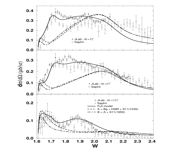
a) S-wave resonances

In Fig.1 the dashed curves (A) show the sum of contributions from the background terms (Bg), High Mass Resonances (HMR), and the $S_{11}$(1535) resonance. A peak appears at all three angles close to threshold. The other two terms (specially HMR) have large contributions at forward angles and higher energies. The second $S_{11}$ resonance, which comes in, due to the configuration mixing, suppresses the effect of the first resonance and affects very slightly higher energy region (curves B).

Figure 2: Same as Fig. 1, but with contributions from P-wave resonances shown.

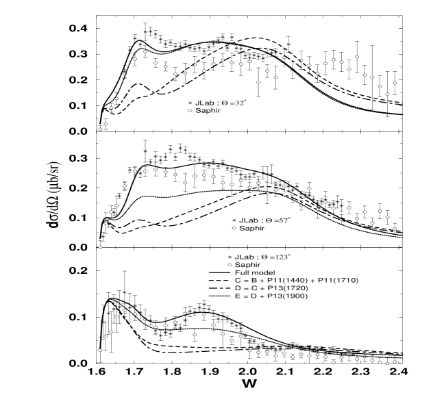
b) P-wave resonances

The Roper resonance, being far below threshold and in spite of its large width, has no significant contribution. The $P_{11}$(1710) introduces a tiny structure at forward angles around $W\approx$ 1.7 GeV (curves C). The first $P_{13}$ enhances that structure (curves D). The most dramatic effect is due to the $P_{13}$(1900). At most forward angle, the curve E gives almost the same result as the full calculation, especially above $W\approx$1.8 GeV. At the two other angles, roughly half of the cross section is obtained in the 1.7 $\leq W\leq$ 2.1 GeV region. Below $W\approx$ 1.8 GeV, we witness strong interference phenomena, while the effects around $W\approx$ 1.9 GeV correspond to the (almost) on-shell contributions.

Figure 3: Same as Fig. 1, but with contributions from $D_{13}$-resonances shown.

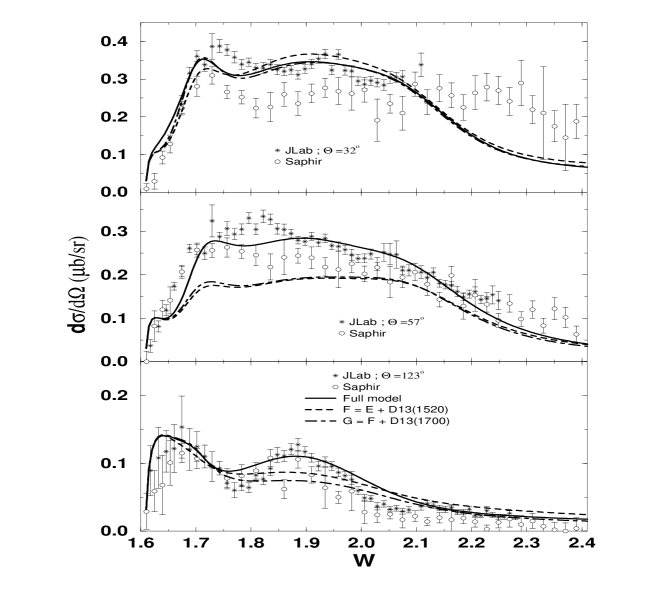
c) Spin-3/2 D-wave resonances

The $D_{13}$(1520) and $D_{13}$(1700) affect slightly the extreme angles results. The first one (curves F) enhances the cross sections corresponding to the curves E, while the second one suppresses them with comparable strength. The final curves G are almost identical to the curves E. Here, $D_{13}$(1700) contributes again due to the configuration mixing mechanism.

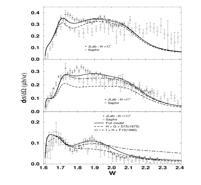
d) Spin-5/2 D- & F-wave resonances

The $D_{15}$(1675) shows a noticeable contribution only at the most forward angle (curves H). In the contrary, the effects of the $F_{15}$(1680) appear at two other angles (curves I), and become very important at the most backward angle above $W\approx$ 1.8 GeV. Here also we are in the presence of strong interference mechanisms. Finally, the addition of the $F_{15}$(2000) leads to the full curves, allowing us to reproduce data around $W\approx$ 1.9 GeV, as well as the high energy part of the data at the most backward angle.

Figure 4: Same as Fig. 1, but with contributions from $D_{15}$- & $F_{15}$-resonances depicted.

4 Summary and Concluding remarks

In this contribution, the preliminary results of a chiral constituent quark model have been compared with the most recent excitation functions measurements at 3 angles from CLAS[1] and SAPHIR[2]. The discrepencies between the two data set do not allow to reach strong conclusions on the underlying reaction mechanism. However, the role played by higher spin and higher mass resonances, such as $P_{11}$(1900), $F_{15}$(1680), and $F_{15}$(2000) is established. The obtained model reproduces the single polarization asymmetries from CLAS and LEPS. Those results, shown during the Conference, could not be reproduced here because of lack of space.

To go further, several directions deserve attention and effort. From experimental side, single and double polarization data, e.g. being analyzed by the GRAAL collaboration, will very likely shed a valuable light on the reaction mechanism issues. From theoretical point of view, the following points need to be studied[24]:

i) The same formalism should be used to interpret the data on the $K^{+}\Sigma^{\circ}$ channel. The forthcoming data from LNS[25] on the $K^{\circ}$ will also put more constraints on the models.

ii) The effect of the third $S_{11}$ resonance, in line with the $\eta p$ final state investigations[20], has to be studied for the strangeness channels. If this latter resonance has a molecular structure[26], it should show up very clearly in the strangeness production processes.

iii) Given that the SAPHIR data go beyond the resonance region, to explain highest energy data, one needs very likely to introduce the t-channel contributions. For the same reason, explicit investigation of resonances with spin $\geq$ 7/2 might be relevant.

Once such improvements to the quark models are ensured, then the coupled channel effects[18] have to be considered. The couplings extracted within the coupled-channel formalisms can then be embodied in the isobaric approaches, including a reasonable number of resonances, to produce the needed elementary operators and study the electroproduction on both proton and nuclei.

It is a pleasure for me to thank the organizers for their kind invitation to this very stimulating conference. I am indebted to K.H. Glander and R. Schumacher for having provided me with the SAPHIR and CLAS data, respectively, prior to publication. I am grateful to my collaborators Z. Li and T. Ye.

References

- [1] J.W.C. McNabb et al. (The CLAS Collaboration), nucl-ex/0305028.
- [2] K.H. Glander et al. (The SAPHIR Collaboration), nucl-ex/0308025, to appear in Eur. Phys. J. A.
- [3] R.G.T. Zegers et al. (The LEPS Collaboration), Phys. Rev. Lett. 91, 092001 (2003).
- [4] R.M. Mohring et al. (The E93018 Collaboration), Phys. Rev. C 67, 055205 (2003); D.S. Carman et al. (The CLAS Collaboration), Phys. Rev. Lett. 90, 131804 (2003).
- [5] R.A. Adelseck and B. Saghai, Phys. Rev. C 42, 108 (1990).
- [6] H. Thom et al., Phys. Rev. Lett. 11, 434 (1963); H. Thom, Phys. Rev. 151, 1322 (1966).
- [7] S.S. Hsiao and S.R. Cotanch, Phys. Rev. C 28, 1668 (1983); R.A. Adelseck, C. Bennhold, L.E. Wright, Phys. Rev. C 32, 1681 (1985).
- [8] R.A. Williams, C.R. Ji, S.R. Cotanch, Phys. Rev. C 46, 1617 (1992).
- [9] J.C. David, C. Fayard, G.H. Lamot, B. Saghai, Phys. Rev. C 53, 2613 (1996).
- [10] T. Mizutani, C. Fayard, G.H. Lamot, B. Saghai, Phys. Rev. C 58, 75 (1998).
- [11] T. Mart and C. Bennhold, Phys. Rev. C 61, 012201 (2000).
- [12] B.S. Han, M.K. Cheoun, K.S. Kim, I-T. Cheon, Nucl. Phys. A691, 713 (2001).
- [13] S. Janssen, D.G. Ireland, J. Ryckebusch, Phys. Lett. B562, 51 (2003); S. Janssen, J. Ryckebusch, T. Van Cauteren, Phys. Rev. C 67, 052201 (2003).
- [14] R.M. Davidson and R. Workman, Phys. Rev. C 67, 058201 (2001).
- [15] K. Hagiwara et al., Particle Data Group, Phys. Rev. D 66, 010001 (2002).
- [16] T.S.H. Lee, V.G.J. Stoks, B. Saghai, C. Fayard, Nucl. Phys. A639, 247 (1998); T.S.H. Lee, Zhong-Yu Ma, H. Toki, B. Saghai, Phys. Rev. C 58, 1551 (1998); L.J. Abu-Raddad, J. Piekarewicz, Phys. Rev. C 61, 014604 (2000); F.X. Lee, T. Mart, C. Bennhold, L.E. Wright, Nucl. Phys. A695, 237 (2001); P. Bydzovsky et al. nucl-th/0305039; M. Sotona, these Proceedings; T. Motoba, these Proceedings.
- [17] J. Caro Ramon, N. Kaiser, S. Wetzel, W. Weise, Nucl. Phys. A672, 249 (2000); J.A. Oller, E. Oset, A. Ramos, Prog. Part. Nucl. Phys. 45 157, (2000); G. Penner and U. Mosel, Phys. Rev. C 66, 055212 (2002).
- [18] W.-T Chiang, F. Tabakin, T.S.H. Lee, B. Saghai, Phys. Lett. B517, 101 (2001).
- [19] A. Manohar and H. Georgi, Nucl. Phys. B234, 189 (1984).
- [20] B. Saghai and Z. Li, Eur. Phys. J. A11, 217 (2001).
- [21] Z. Li, H. Ye, M. Lu, Phys. Rev. C 56, 1099 (1997).
- [22] Z. Li and B. Saghai, Nucl. Phys. A 644, 345 (1998).
- [23] N. Isgur and G. Karl, Phys. Lett. B72, 109 (1977); N. Isgur, G. Karl, R. Koniuk, Phys. Rev. Lett. 41, 1269 (1978); J. Chimza and G. Karl, Phys. Rev. D 68 054007 (2003).
- [24] Z. Li, B. Saghai, T. Ye, in progress.
- [25] T. Takahashi et al. (The NKS Collaboration), these Proceedings.
- [26] Z. Li and R. Workman, Phys. Rev. C 53, R549 (1996).