Analysis of anisotropic flow with Lee-Yang zeroes

Abstract

We present a new method to extract anisotropic flow in heavy ion collisions from the genuine correlation among a large number of particles. Anisotropic flow is obtained from the zeroes in the complex plane of a generating function of azimuthal correlations, in close analogy with the theory of phase transitions by Lee and Yang. Flow is first estimated globally, i.e., averaged over the phase space covered by the detector, and then differentially, as a function of transverse momentum and rapidity for identified particles. The corresponding estimates are less biased by nonflow correlations than with any other method. The practical implementation of the method is rather straightforward. Furthermore, it automatically takes into account most corrections due to azimuthal anisotropies in the detector acceptance. The main limitation of the method is statistical errors, which can be significantly larger than with the “standard” method of flow analysis if the flow and/or the event multiplicities are too small. In practice, we expect this to be the most accurate method to analyze directed and elliptic flow in fixed-target heavy-ion collisions between 100 MeV and 10 GeV per nucleon (at the Darmstadt SIS synchrotron and the Brookhaven Alternating Gradient Synchrotron), and elliptic flow at ultrarelativistic energies (at the Brookhaven Relativistic Heavy Ion Collider, and the forthcoming Large Hadron Collider at CERN).

I Introduction

Study of anisotropic flow of particles Reviews produced in relativistic heavy-ion collisions has emerged as an important tool to probe the early history, especially the thermalization, of the dense fireball produced in these collisions. Anisotropic flow means that the azimuthal distribution of particles produced in non-central collisions, measured with respect to the direction of impact parameter, is not flat. This is characterized by the Fourier harmonics Voloshin:1996mz :

$$v_{n}\equiv\left\langle\cos n(\phi-\Phi_{R})\right\rangle,$$ (1)

where $\phi$ denotes the azimuthal angle of an outgoing particle, $\Phi_{R}$ is the azimuthal angle of the impact parameter ($\Phi_{R}$ is also called the orientation of the reaction plane), $n$ is a positive integer, and angular brackets denote an average over many particles belonging to some phase-space region, and over many events. Throughout this paper, we assume that colliding nuclei are spherical and parity is conserved: then, the system is symmetric with respect to the reaction plane and $\left\langle\sin n(\phi-\Phi_{R})\right\rangle$ vanishes for all $n$. The two lowest harmonics $v_{1}$ and $v_{2}$ are named directed and elliptic flows. They have been studied extensively over the last several years, with reference to the wealth of data produced at GANIL Cussol:2001df , at the Darmstadt SIS synchrotron FOPI ; Andronic:2000cx ; Andronic:2001sw ; Taranenko:1999yh , the Brookhaven Alternating Gradient Synchrotron (AGS) Jain:1995cm ; Barrette:xr ; E877 ; Pinkenburg:1999ya ; Liu:2000am ; E895 ; Chung:2001qr , and the Super Proton Synchrotron (SPS) at CERN CERES ; Agakichiev:2003gg ; NA49 ; NA49new ; WA98 , as well as the new and upcoming data from the Relativistic Heavy Ion Collider (RHIC) at Brookhaven PHENIX ; PHENIX200 ; PHOBOS ; STAR2p ; Adler:2002pu ; Adler:2002ct .

Since the reference direction $\Phi_{R}$ is not known experimentally, measuring $v_{n}$ is a difficult task. An alternate idea is to extract it from the interparticle correlations which arise indirectly due to the correlation of each particle with the reaction plane. However, standard methods of correlating a particle with an estimate of the reaction plane Danielewicz:hn ; Ollitrault:1997di ; Poskanzer:1998yz , or of correlating two particles with each other Wang:1991qh were shown to be inadequate at ultrarelativistic SPS energies Dinh:1999mn due to the smallness of the flow, and the comparatively large magnitude of “nonflow” correlations Poskanzer:1998yz ; Ollitrault:dy due to transverse momentum conservation, resonance decays, etc., which are usually neglected in these methods. At the higher RHIC energies, it was argued that nonflow correlations due to minijets could even dominate the measured correlations Kovchegov:2002nf .

These shortcomings of conventional methods motivated the development of new methods based on a cumulant expansion of multiparticle correlations Borghini:2000sa ; Borghini:2001vi ; Borghini:2002vp . The cumulant of the $k$-particle correlation, where $k$ is a positive integer, isolates the genuine $k$-particle correlation by subtracting the contribution of lower-order correlations. Nonflow correlations, which generally involve only a small number of particles (typically, two or three in the case of resonance decays, possibly more in the case of minijets) contribute little to the cumulant if $k$ is large enough. Note that this is also true for correlations from global momentum conservation, although the latter involves all particles Borghini:2003ur . On the other hand, anisotropic flow is a genuine collective effect, in the following specific sense: in a given event, all azimuthal angles are correlated with the reaction plane azimuth $\Phi_{R}$, which varies randomly from one event to the other. In the laboratory frame, where $\Phi_{R}$ is unknown, this results in azimuthal correlations between all particles, or at least a significant fraction of the particles. Therefore, unlike nonflow correlations, anisotropic flow contributes to cumulants of all orders $k$. Neglecting the contribution of nonflow correlations to the cumulant, one thus obtains an estimate of $v_{n}$, which was denoted by $v_{n}\{k\}$ in Ref. Borghini:2001vi , and becomes more and more reliable as $k$ increases.

Cumulants of four-particle correlations were first used to measure elliptic flow at RHIC Adler:2002pu . However, it was argued that experimental results could still be explained by nonflow correlations alone Kovchegov:2002cd at this order. Higher-order cumulants, of up to 8 particles, were constructed at SPS NA49new , and provide the first quantitative evidence for anisotropic flow at ultrarelativistic energies. In practice, the cumulant of 8-particle correlations is obtained by evaluating numerically the 8^th derivative of a generating function. This is rather tedious and numerically hazardous.

In this paper, we propose to study directly the large-order behavior of the cumulant expansion, rather than computing explicitly cumulants at a given order. Correlating a large number of particles is the most natural way of studying genuine collective motion in the system. Furthermore, finding the large-order behavior turns out to be simpler in practice than working at a given, finite order. As we shall see, the large-order behavior is determined by the location of the zeroes of a generating function in the complex plane bbo . In this respect, our method is in close analogy with the theory of phase transitions formulated 50 years ago by Lee and Yang Yang:be ; Lee:1952ig : at the critical point, long-range correlations appear in the system; as a consequence, the zeroes of the grand partition function come closer and closer to the real axis as the size of the system increases. A similar phenomenon occurs here, and anisotropic flow appears as formally equivalent to a first order phase transition.

The idea of studying anisotropic flow through the correlation of a large number of particles is not new. The same idea underlies global event analyses through a three-dimensional sphericity tensor Danielewicz:we , which led to the first observation of collective flow at Bevalac Gustafsson:ka . A similar two-dimensional analysis, restricted to the transverse plane Voloshin:1996mz ; Ollitrault:bk , led to the discovery of flow at the Brookhaven Alternating Gradient Synchrotron (AGS) Barrette:xr . With these methods, however, one could not study anisotropic flow differentially, that is, as a function of transverse momentum and rapidity for identified particles. This is why they were soon superseded by the more detailed, although less reliable, two-particle methods. One of our important results is that the method presented in this paper also allows one to analyze differential flow, and its implementation is rather straightforward.

The paper is organized as follows. In Sec. II we present in a self-contained manner our recipes to calculate the “asymptotic” integrated and differential flows. The derivations of these results are given in Sec. III, where they are related with the Lee-Yang theory. The remaining Sections are devoted to detailed discussions of the various sources of error. It is now well known that (even when anisotropic flow is absent) “nonflow” correlations may give a spurious result when the various techniques of flow analysis are applied. In Sec. IV, we discuss the magnitude of this spurious flow, and show that it is significantly smaller than with any previous method: the main point of this paper is that the present method is the most efficient way to disentangle anisotropic flow from other effects. When anisotropic flow is present in the system, nonflow correlations produce a systematic error, which is estimated in Sec. V. The effect of fluctuations of flow (due for instance to variations of impact parameter in a given centrality bin) on our results is discussed in Sec. VI. Statistical uncertainties on the flow estimates within the method are computed in Sec. VII. They are the main practical limitation of our method. Acceptance corrections due to limited azimuthal coverage of the detectors are discussed in Sec. VIII. Section IX is a summary. Finally, four appendices are devoted to further discussions and calculations.

II Recipes for extracting genuine collective flow

In this Section, we show how to obtain an estimate of the flow $v_{n}$ from the genuine correlation among a large number of particles. The fact that azimuthal angles of outgoing particles are correlated with the azimuth of the reaction plane $\Phi_{R}$ allows one to construct in each event a reference direction, which is called an “estimate of the reaction plane” in the standard Danielewicz-Odyniec method Danielewicz:hn . This direction is defined by the flow vector of the event, as recalled in Sec. II.1. Note that, unlike other multiparticle methods Borghini:2001vi , the present one is based on the flow vector.

The flow analysis then proceeds in two successive steps. The first one is to estimate how the flow vector is correlated with the true reaction plane. More precisely, we estimate the mean projection of the flow vector on the true reaction plane. This quantity is a weighted sum of the individual flows $v_{n}$ of all particles over phase space, which we call “integrated flow” and denote by $V_{n}$. The method used to estimate $V_{n}$ experimentally is described in Sec. II.2. This first step is the equivalent of the subevent method in the standard flow analysis, from which one estimates the event-plane resolution. Here however, as well as in the cumulant method based on the flow vector Borghini:2000sa , subevents are not needed.

The second step in the analysis is to use this reference integrated flow to analyze “differential flow,” i.e., flow in a restricted phase-space window (e.g., as a function of transverse momentum and rapidity for a given particle type), which is the goal of the flow analysis. When analyzing a $p$-th harmonic of the differential flow ($v_{p}$), the flow vector can be chosen in the same harmonic $p$, or in a lower harmonic $n$ whose $p$ is a multiple. One chooses the option which yields the best accuracy. For instance, differential elliptic flow $v_{2}$ can be analyzed using as a reference either the integrated elliptic flow (at ultrarelativistic energies CERES ; NA49 ; NA49new ; WA98 ; PHENIX ; PHENIX200 ; PHOBOS ; STAR2p ; Adler:2002pu ) or the integrated directed flow (at lower energies Demoulins:ac ; Andronic:2000cx ; Chung:2001qr ).

The method to extract differential flow is described in Sec. II.3. Following the notations of Refs. Borghini:2000sa ; Borghini:2001vi , differential flow in the Fourier harmonic $p$ will be denoted by $v^{\prime}_{p}$. The estimates of $V_{n}$ and $v^{\prime}_{p}$ obtained with the present method will be denoted by $V_{n}\{\infty\}$ and $v^{\prime}_{p}\{\infty\}$, respectively, where the symbol $\infty$ means that it corresponds to the large-order behavior of the cumulant expansion, as will be shown in Sec. III.

Section II.4 discusses briefly acceptance issues arising when the detector does not have full azimuthal coverage. Section II.5 shortly deals with statistical errors, which are the main limitation of our method. Both issues are discussed in more detail in Sec. VIII and Sec. VII, respectively.

II.1 The flow vector

The first step of the flow analysis is to evaluate, for each event, the flow vector of the event. It is a two-dimensional vector ${\bf Q}=(Q_{x},Q_{y})$ defined as

$$Q_{x} = \sum_{j=1}^{M}w_{j}\,\cos(n\phi_{j})$$ (2)

$$Q_{y} = \sum_{j=1}^{M}w_{j}\,\sin(n\phi_{j}),$$ (3)

where $n$ is the Fourier harmonic under study ($n=1$ for directed flow, $n=2$ for elliptic flow), the sum runs over all detected particles, $M$ is the observed multiplicity of the event, $\phi_{j}$ are the azimuthal angles of the particles measured with respect to a fixed direction in the laboratory.

The coefficients $w_{j}$ in Eq. (2) are weights depending on transverse momentum, particle mass and rapidity. The best choice of $w_{j}$ is that leading to the smallest statistical error, by maximizing the flow signal. The weight should ideally be proportional to the flow itself, $w_{j}(p_{T},y)\propto v_{n}(p_{T},y)$ Borghini:2000sa . Otherwise, reasonable choices are $w\propto y-y_{\rm cm}$, i.e., the rapidity in the center-of-mass frame, for directed flow, and $w=p_{T}$ for elliptic flow.

When comparing events with different multiplicities $M$, one may in addition have weights depending on $M$. Weights proportional to $1/\sqrt{M}$ were used in Ref. Borghini:2000sa , and proportional to $1/M$ in Ref. Borghini:2001vi , to minimize the effect of multiplicity fluctuations. This complication is unnecessary here. This issue is discussed in Appendix B.

The discussions in this paper will be illustrated by explicit numerical and analytical examples, in which we choose unit weights $w_{j}=1$, for the sake of simplicity.

The flow vector was first introduced in Ref. Danielewicz:hn . The azimuthal angle $n\Phi_{n}$ of ${\bf Q}$ is conventionally used in the analysis of anisotropic flow Poskanzer:1998yz in order to estimate the orientation of the reaction plane of the event.

Our method uses the projection of ${\bf Q}$ on a fixed, arbitrary direction making an angle $n\theta$ with respect to the $x$-axis. We denote this projection by $Q^{\theta}$:

$$Q^{\theta} \equiv Q_{x}\cos(n\theta)+Q_{y}\sin(n\theta)$$ (4)

$$= \sum_{j=1}^{M}w_{j}\,\cos(n(\phi_{j}-\theta)).$$ (5)

As we shall see, the whole flow analysis can in principle be performed using this projection of the flow vector on a fixed direction. One thus obtains an estimate of the integrated flow $V_{n}^{\theta}\{\infty\}$ (Sec. II.2), which is then used as a reference to derive an estimate of the differential flow $v^{\prime\theta}_{mn}\{\infty\}$ (Sec. II.3).

In practice, however, one should perform the analysis for several equally spaced values of $\theta$, typically $\theta=(k/p)(\pi/n)$ with $k=0,\ldots,p-1$ and $p=4$ or 5. This gives several values of $V_{n}^{\theta}\{\infty\}$ and $v^{\prime\theta}_{mn}\{\infty\}$, which are then averaged over $\theta$. This yields our final estimates of integrated flow, $V_{n}\{\infty\}$, and differential flow, $v^{\prime}_{mn}\{\infty\}$. As we shall see in Sec. VII, they have smaller statistical error bars than each individual $V_{n}^{\theta}\{\infty\}$ and $v^{\prime\theta}_{mn}\{\infty\}$.

II.2 Integrated flow

Integrated flow is defined as the average value of the flow vector projected on the unit vector with angle $n\Phi_{R}$ (for $n=1$, this is the reaction plane):

$$V_{n} \equiv \left\langle Q_{x}\,\cos(n\Phi_{R})+Q_{y}\,\sin(n\Phi_{R})\right\rangle$$ (6)

$$= \left\langle Q^{\Phi_{R}}\right\rangle,$$ (7)

where we have used the notation introduced in Eq. (4). This quantity was denoted by $\bar{Q}$ in Ref. Ollitrault:1997di , and by $\left\langle\bf Q\right\rangle$ in Ref. Borghini:2000sa . Note that unlike the flow coefficients $v_{n}$, which are dimensionless, our integrated flow involves the weights present in the flow vector (2), which can have a dimension. Since the flow vector definition involves a sum over all particles, the integrated flow scales like the multiplicity $M$. With unit weights,

$$V_{n}=Mv_{n},$$ (8)

where $v_{n}$ in the right-hand side (rhs) is to be understood as an average over the phase space covered by the detector acceptance, and we have neglected fluctuations of the multiplicity $M$ for simplicity.

Let us now explain how an estimate of $V_{n}$ can be obtained in a real experiment. For a given value of $\theta$, we first define the following generating function, which depends on an arbitrary complex variable $z$:

$$G^{\theta}(z)\equiv\left\{e^{zQ^{\theta}}\right\},$$ (9)

where curly brackets denote an average over a large number of events, $N_{\rm evts}$, with (approximately) the same centrality. This generating function has the symmetry properties

$$G^{\theta+\pi/n}(z)=G^{\theta}(-z)$$ (10)

(following from $Q^{\theta+\pi/n}=-Q^{\theta}$), and

$$[G^{\theta}(z)]^{*}=G^{\theta}(z^{*}),$$ (11)

where the star denotes complex conjugation. The second identity simply expresses that $G^{\theta}(z)$ is real for real $z$. An alternative choice of the generating function is presented in Appendix A.

In order to obtain the integrated flow, one must evaluate $G^{\theta}(z)$ for a large number of values of $z$ on the upper half of the imaginary axis (that is, $z=ir$ with $r$ real and positive). One must then take the modulus [recall that $G^{\theta}(z)$ is a complex number], $\left|G^{\theta}(ir)\right|$, and plot it as a function of $r$. On the imaginary axis, the symmetry properties, Eqs. (10) and (11) translate into the following relations: $G^{\theta+\pi/n}(ir)=G^{\theta}(-ir)=[G^{\theta}(ir)]^{*}$. Taking the modulus, this yields $|G^{\theta+\pi/n}(ir)|=|G^{\theta}(-ir)|=|G^{\theta}(ir)|$. This identity shows that $\theta$ and $\theta+\pi/n$ are equivalent, so that one can restrict $\theta$ to the interval $[0,\pi/n]$. It also shows that $z=ir$ and $z=-ir$ are equivalent, which is the reason why we restrict ourselves to positive $r$ values.

To illustrate the variation of $\left|G^{\theta}(ir)\right|$ as a function of $r$, we have computed it for simulated data. The data set contained $N_{\rm evts}=20000$ events with multiplicity $M=300$. Each event consisted of 10 “differential bins” with equally spaced elliptic flow values ranging from 4.2 to 7.8%, resulting in an average $v_{2}=6\%$, and with a higher flow harmonic $v_{4}=3\%$ for all particles. The flow vector, Eq. (2), was constructed using unit weights $w_{j}=1$ and $n=2$. We assumed that the detector acceptance had perfect azimuthal symmetry. The function $\left|G^{\theta}(ir)\right|$ is shown in Fig. 1 for $\theta=0$. Due to rotational symmetry (for a perfect detector), the behavior would be similar for another value of $\theta$, up to statistical fluctuations. The function $\left|G^{\theta}(ir)\right|$ starts at a value of $1$ for $r=0$, and it then decreases and oscillates.

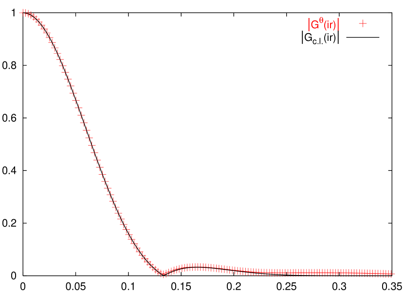
Figure 1: Variation of $\left|G^{\theta}(ir)\right|$ with $r$, for $N_{\rm evts}=20000$ simulated events, with $M=300$ particles per event and a mean elliptic flow $v_{2}=6\%$, to match the typical value in a mid-central Au+Au collision at $\sqrt{s_{{}_{\rm NN}}}=130$ GeV, as analyzed by the STAR Collaboration at RHIC STAR2p . The crosses are the values of $|G^{\theta}(ir)|$ for $\theta=0$. The solid line displays the expected value $|G_{\rm c.l.}(ir)|$ [defined by Eq. (26)].

Our estimate of integrated flow is directly related to the first minimum of $\left|G^{\theta}(ir)\right|$. Let us denote by $r_{0}^{\theta}$ the value of $r$ corresponding to the first minimum. The corresponding estimate of integrated flow is defined as

$$V_{n}^{\theta}\{\infty\}\equiv\frac{j_{01}}{r_{0}^{\theta}},$$ (12)

where $j_{01}\simeq 2.405$ is the first root of the Bessel function $J_{0}(x)$. This result will be justified in Sec. III. As one can see in Fig. 1, the variation of $\left|G^{\theta}(ir)\right|$ near its minimum is quite steep. Therefore, from the numerical point of view, one should rather determine the minimum of the square modulus $\left|G^{\theta}(ir)\right|^{2}$.

As will be shown in Sec. III, the value of $|G^{\theta}(ir)|$ at its minimum would be zero in the limit of an infinite number of events. One can check experimentally that it is compatible with zero within expected statistical fluctuations. Anticipating on Sec. VII.3 [see the discussion following Eq. (82], the following inequality should hold with 95% confidence level:

$$|G^{\theta}(ir_{0}^{\theta})|<\frac{2}{\sqrt{N_{\rm evts}}},$$ (13)

where $N_{\rm evts}$ is the number of events used in the analysis.

Eventually, the final estimate $V_{n}\{\infty\}$ is obtained by averaging $V_{n}^{\theta}\{\infty\}$ over $\theta$:

$$V_{n}\{\infty\}\equiv\frac{1}{p}\sum_{k=0}^{p-1}V_{n}^{k\pi/pn}\{\infty\},$$ (14)

with $p$ typically 4 or 5.

This procedure was applied to the simulated data used for Fig. 1. As stated above, we used constant unit weights $w_{j}=1$ in Eq. (2), so that Eq. (8) holds. Estimates $V_{2}^{\theta}\{\infty\}$ were then computed for many values of $\theta$ (for the sake of illustration, we did not restrict ourselves to 4 or 5 values, as would have been enough, see Sec. VII.5). Since we assumed that the detector is perfect, $V_{2}^{\theta}\{\infty\}$ should be independent of $\theta$, up to statistical fluctuations. The results of the analysis are displayed in Fig. 2, where $V_{2}^{\theta}\{\infty\}/M$ is plotted as a function of $\theta$. The $\theta$-dependence is smooth and has a small amplitude. The estimates for $\theta=0$ and $\theta=\pi/2$ coincide, as expected from the ($\pi/n$)-periodicity.

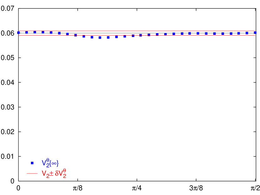
Figure 2: Reconstruction of integrated flow. The simulated data and the definition of the flow vector are the same as in Fig. 1. The plot shows $V_{2}^{\theta}\{\infty\}/M$ as a function of $\theta$. The lines display the expected value with statistical error bars calculated as explained in Sec. VII.5.

The salient feature in Fig. 2 is the accuracy of the reconstruction of the input. As will be shown in Sec. VII.5, the expected statistical uncertainty on each individual estimate $V_{2}^{\theta}\{\infty\}/M$ is $0.092\%$. One sees in the figure that most values of $V_{2}^{\theta}\{\infty\}/M$ are within error bars. The expected statistical error bar on the average over $\theta$, $V_{2}\{\infty\}/M$, is $0.051\%$ (see Sec. VII.5), i.e., smaller than the statistical error on each $V_{2}^{\theta}\{\infty\}$ by almost a factor of 2. We obtain $V_{2}\{\infty\}/M=5.95\%$, in perfect agreement with the input value $v_{2}=6\%$.

Finally, let us mention that, like every other method of flow analysis, the present one cannot determine the sign of integrated flow: the estimate given by Eq. (12), and its average over $\theta$, are positive by definition, while the integrated flow defined by Eq. (6) can be negative. The reason is that our procedure is unchanged if the sign of the flow vector is changed in all events [this amounts to changing $z$ into $-z$ in Eq. (9)], while this transformation changes the sign of the integrated flow $V_{n}$. Strictly speaking, $V_{n}\{\infty\}$ should therefore be considered an estimate of $|V_{n}|$, rather than $V_{n}$. The sign must be determined independently, or assumed.

II.3 Differential flow

Using an estimate of integrated flow in the Fourier harmonic $n$, one can analyze differential flow in harmonics which are multiples of $n$, i.e., $mn$, where $m$ is an arbitrary integer. Following the notations of Ref. Borghini:2001vi , we denote by $v^{\prime}_{mn}$ the differential flow corresponding to a given phase-space window in this harmonic. We call “proton” any particle belonging to the phase-space window under study, and denote by $\psi$ its azimuthal angle.

For a given value of the angle $\theta$, the corresponding estimate of differential flow $v^{\prime}_{mn}$ is given by:

$$\frac{v^{\prime\theta}_{mn}\{\infty\}}{V^{\theta}_{n}\{\infty\}}\equiv\frac{J_{1}(j_{01})}{J_{m}(j_{01})}\,{\rm Re}\!\left(\frac{\left\{\cos[mn(\psi-\theta)]\,e^{ir_{0}^{\theta}Q^{\theta}}\right\}}{i^{m-1}\left\{Q^{\theta}e^{ir_{0}^{\theta}Q^{\theta}}\right\}}\right),$$ (15)

where ${\rm Re}$ denotes the real part, and $r_{0}^{\theta}$ has been defined in Sec. II.2. Two different sample averages appear in the rhs of this equation: the numerator is an average over all “protons” in all events, while the denominator is an average over events. Note that the term $\left\{Q^{\theta}e^{ir_{0}^{\theta}Q^{\theta}}\right\}$ in the denominator is in fact the derivative of $G^{\theta}(z)$ with respect to $z$ [see Eq. (9)], evaluated at $z=ir_{0}^{\theta}$.

The numerical coefficient $J_{1}(j_{01})/J_{m}(j_{01})$ in Eq. (15) involves the ratio of two Bessel functions. It takes the values $1$ for $m=1$ and $j_{01}/2\simeq 1.202$ for $m=2$. In the case $m=1$ (lowest harmonic), one recovers the estimate of integrated flow $V^{\theta}_{n}\{\infty\}$ by integrating the corresponding estimate of differential flow $v^{\prime\theta}_{n}\{\infty\}$, over all phase space, which amounts to summing over $\psi$ in the rhs of Eq. (15), with the appropriate weighting.

If $\cos$ is replaced by $\sin$ in the numerator of the rhs of Eq. (15), the result should be zero within statistical errors if parity is conserved. This can easily be checked experimentally. A non-zero result could be a signature of parity violation Kharzeev:1998kz ; Voloshin:2000xf . This issue will not be discussed further in this paper.

As in the case of integrated flow, the estimates of differential flow given by Eq. (15) have a periodicity property, namely $v^{\prime\,\theta+\pi/n}_{mn}\{\infty\}=v^{\prime\theta}_{mn}\{\infty\}$. Indeed, changing $\theta$ into $\theta+\pi/n$ amounts to replacing the term in brackets by its complex conjugate, which does not affect the value of the real part. As above, the estimates $v^{\prime\theta}_{mn}\{\infty\}$ must be averaged over $\theta$ in the interval $[0,\pi/n]$, in order to obtain an estimate with a reduced statistical uncertainty.

Please note that there appear “autocorrelations” in the numerator of Eq. (15): one correlates the angle $\psi$ with $Q^{\theta}$, which itself involves in general the angle $\psi$ [since the summation in Eq. (2) runs over all detected particles]. In the standard method of flow analysis Danielewicz:hn ; Poskanzer:1998yz , autocorrelations are large, so that one has to remove the particle with angle $\psi$ from the flow vector. Here, however, autocorrelations do not produce a spurious flow by themselves, as will be explained in Sec. III.5.4. For the lowest harmonic $v^{\prime}_{n}$, they lead to a very small correction and need not be subtracted.  For higher harmonics $v^{\prime}_{2n}$, $v^{\prime}_{3n}$…, errors due to autocorrelations are larger so that one may prefer to subtract them. However, errors of the same order of magnitude are generally expected from nonflow correlations. We come back to this issue in Sec. V.2.

Figure 3 displays the result of the analysis of the same Monte-Carlo simulation as in Figs. 1 and 2, using a detector with perfect azimuthal symmetry. We present the differential flow results in “bin 8,” corresponding to input values of $v^{\prime}_{2}=7\%$, $v^{\prime}_{4}=3\%$, and an average proton number of approximately 30 per event, i.e., a total number of protons $N^{\prime}\simeq 6\times 10^{5}$. Two different analyses were performed. The first one followed the procedure presented in this Section. In a second analysis, we corrected for autocorrelations, subtracting the contribution of the proton with angle $\psi$ from the flow vector before multiplying $\cos[mn(\psi-\theta)]$ by $e^{ir_{0}^{\theta}Q^{\theta}}$ in the numerator of Eq. (15). One sees in Fig. 3 that the $v^{\prime}_{2}$ result is essentially insensitive to autocorrelations. We shall see in Sec. VII.6 that the expected statistical errors on $v_{2}^{\prime\theta}\{\infty\}$ and $v_{4}^{\prime\theta}\{\infty\}$ are 0.47% and 0.57%, respectively. Values mostly fall within the expected range around the input value, except for $v^{\prime}_{4}$ when autocorrelations are not subtracted.

After averaging over $\theta$, one obtains $v^{\prime}_{2}\{\infty\}=7.00\pm 0.26\%$ and $v^{\prime}_{4}\{\infty\}=3.60\pm 0.29\%$ with autocorrelations and $v^{\prime}_{2}\{\infty\}=7.20\pm 0.26\%$, $v^{\prime}_{4}\{\infty\}=3.03\pm 0.29\%$ when autocorrelations are removed, where statistical uncertainties have been computed with the help of formulas given in Sec. VII.6. For the lower harmonic $v^{\prime}_{2}$, results are in good agreement with the input value $v^{\prime}_{2}=7\%$, whether or not autocorrelations are subtracted. For the higher harmonic $v^{\prime}_{4}$, a discrepancy with the input value $v^{\prime}_{4}=3\%$ appears when autocorrelations are not subtracted. This error will be evaluated analytically in Sec. V.2.

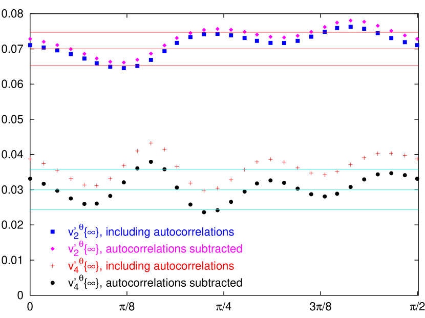
Figure 3: Reconstruction of differential flow. The simulated data and the definition of the flow vector are the same as in Figs. 1 and 2. The plot shows $v_{2}^{\prime\theta}\{\infty\}$ and $v_{4}^{\prime\theta}\{\infty\}$ as a function of $\theta$. Squares: $v_{2}^{\prime\theta}\{\infty\}$ with autocorrelations. Diamonds: $v_{2}^{\prime\theta}\{\infty\}$ with autocorrelations removed. Crosses: $v_{4}^{\prime\theta}\{\infty\}$ with autocorrelations. Circles: $v_{4}^{\prime\theta}\{\infty\}$ with autocorrelations removed. The solid lines display the expected value with statistical error bars calculated as explained in Sec. VII.6.

Like other methods of flow analysis, the present procedure has a global sign ambiguity, due to the fact that the sign of the integrated flow $V_{n}$ cannot be reconstructed. In Eq. (15), both $V_{n}^{\theta}\{\infty\}$ and $r_{0}^{\theta}$ are positive. If the true integrated flow $V_{n}$ is also positive, then our estimate $v^{\prime\theta}_{mn}\{\infty\}$ has the correct sign. If, on the other hand, $V_{n}$ is negative, then $v^{\prime\theta}_{mn}\{\infty\}$ should be multiplied by $(-1)^{m}$. [equivalently, one can change the sign of $V_{n}^{\theta}\{\infty\}$ and $r_{0}^{\theta}$ in Eq. (15)].

II.4 Acceptance corrections

The standard event-plane analysis requires that the flow vector ${\bf Q}$ has a perfectly isotropic distribution in azimuth. Since real detectors are not perfect, this requires one to use various flattening procedures Poskanzer:1998yz . One of the nice features of the cumulant expansion is that it isolates physical correlations by subtracting out the contribution of detector asymmetries Borghini:2000sa . The same occurs here, so that flattening procedures are not needed. Detector asymmetries can never produce a spurious flow by themselves with the method described above. This holds even if the detector has a very limited azimuthal coverage.

In Sec. VIII, we demonstrate that the effects of strong azimuthal asymmetries in a detector are twofold. First, the estimates $V_{2}^{\theta}\{\infty\}$ depend on $\theta$ [see Eq. (122)]. Second, the average estimate $V_{2}\{\infty\}$ does not exactly coincide with the true value, but differs by a multiplicative coefficient (which also controls the $\theta$-dependence of $V_{2}^{\theta}\{\infty\}$). In most cases, however, this coefficient is so close to unity that correcting for it is not even necessary.

This is illustrated by Fig. 4: we analyzed a simulated data set with similar statistics as that of Figs. 1–3, namely 20000 events of 300 emitted particles, with an average elliptic flow $v_{2}=6\%$ (but now a vanishing $v_{4}$). We assumed that the detector had a blind angle of 60 degrees, i.e., that one sixth of the azimuthal coverage is missing. We can clearly see the oscillation of $V_{2}^{\theta}\{\infty\}$ as a function of $\theta$. After averaging over $\theta$, however, we find $V_{2}\{\infty\}/\left\langle M\right\rangle=6.004\pm 0.066\%$, where $\left\langle M\right\rangle$ denotes the mean multiplicity of detected particles,  in perfect agreement with the input value $v_{2}=6\%$. Note that the statistical error bar is slightly larger than in Fig. 2 due to the reduced multiplicity ($\left\langle M\right\rangle=250$ instead of 300). With this particular detector configuration, the analytical calculation presented in Sec. VIII shows that the reconstructed $V_{2}\{\infty\}$ should be divided by $1.0068$ in order to take detector effects into account [see Eq. (123)], a very small correction indeed.

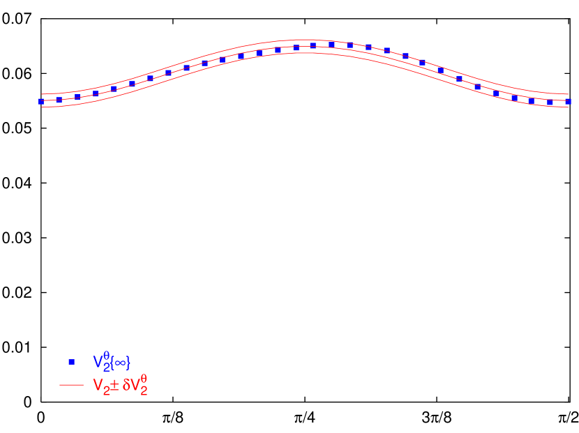
Figure 4: Reconstruction of integrated flow, with a detector which does not detect particles with $150^{\circ}<\phi<210^{\circ}$. The simulated data and the definition of the flow vector are the same as in Fig. 1. The plot shows $V_{2}^{\theta}\{\infty\}/\left\langle M\right\rangle$ as a function of $\theta$. The lines display the theoretical value taking into account detector effects, Eq. (122), with statistical error bars.

Similarly, acceptance inefficiencies have the same two effects on the differential flow estimates obtained with the present method. Thus, $v^{\prime\theta}_{mn}\{\infty\}$ becomes $\theta$-dependent, while $v^{\prime}_{mn}\{\infty\}$ differs from $v^{\prime}_{mn}$ by a multiplicative factor, see Sec. VIII.

Finally, let us emphasize that since the method automatically takes into account most detector asymmetries, it is important to take as input in the construction of the generating function, Eq. (9), the azimuthal angles of the particles exactly as they are measured in the laboratory: flattening procedures are useless here, and might even bias the analysis.

II.5 When is the method applicable?

As we shall demonstrate in the following Sections, the main limitation of the method arises from statistical errors, while systematic errors inherent to the method are under good control. In Sec. VII, we shall see that statistical errors depend on the so-called “resolution parameter” $\chi$. Referring the reader to Sec. VII.1 for further details on this parameter, and in particular on its experimental determination, we simply want to recall here that it is roughly given by $\chi\simeq v_{n}\sqrt{M}$, where $M$ is the typical number of detected particles per event, and $v_{n}$ the typical magnitude of the flow.

Compared to other methods of flow analysis, statistical errors depend very strongly on $\chi$. This is because our method involves the correlation between a large number of particles. It is therefore important to use as many particles as possible in constructing the flow vector, so as to maximize $\chi$. In particular, since our method is very stable with respect to effects of detector acceptance as explained above, one should not do any cuts in phase space. Furthermore, since the method is also stable with respect to “nonflow” correlations, one should not worry about possible “double countings” due to multiple hits or showering effects in the detector. Most current heavy ion experiments consist of several detectors of various types (calorimeters, tracking chambers) covering various regions of phase space (central rapidity, forward/backward rapidity). It is not common in the flow analysis to combine the information from different detectors in constructing the flow vector of the event. Here, it is important to do so: even a few additional particles may result in a significant decrease of the statistical error. Finally, properly chosen weights can significantly increase the value of the resolution parameter $\chi$.

An over-simplified rule of thumb, which emphasizes the role of $\chi$ would be the following:

• if $\chi>1$, the statistical error on the flow is not significantly larger than with the standard method (by a factor of at most 2, see Tables 3, 6 and 7), while systematic errors due to nonflow effects are much smaller. Thus, the present method should be used, and statistics will not be a problem;

• if $0.5<\chi<1$, the method can be used, but it really is most important to optimize weights, so as to increase $\chi$, possibly by performing two analyses of the same data sets: in the first analysis, adopting (educated) guesses for the weights; and in the second pass, using as weights $w_{j}$ the differential flow values obtained in the first analysis;

• if $\chi<0.5$, statistical errors are too large, and the present method cannot be used; increasing the number of events barely helps here; in this case, one should use the cumulant methods of Refs. Borghini:2001vi ; Borghini:2002vp , which still apply if the number of events is large enough NA49new .

III Collective flow and zeroes of the generating function

Let us now justify the procedure presented in the previous Section. We begin with a detailed discussion of our hypotheses (Sec. III.1). In Sec. III.2, we define the cumulants of the distribution of $Q^{\theta}$. We argue that large-order cumulants isolate collective effects from other, nonflow correlations, which generally involve only a few particles. We then show that large-order cumulants are uniquely determined by the location of the zeroes of $G^{\theta}(z)$ in the complex plane of the variable $z$.

Anisotropic flow is a particular case of collective behavior, which can be analyzed using this procedure. For this purpose, we compute the generating function $G^{\theta}(z)$ when anisotropic flow is present (Sec. III.3). This allows us to relate the position of the first zero of $G^{\theta}(z)$ to the integrated flow $V_{n}$. The analogy of this approach with the Lee-Yang theory of phase transitions is shown in Sec. III.4.

The discussion of Secs. III.2 and III.3 is generalized to differential flow in Sec. III.5. The relation of this approach with the cumulant expansion of Refs. Borghini:2000sa ; Borghini:2001vi is described in Appendix B.

III.1 Preliminaries

The derivation of our results relies on the following four hypotheses:

• A) the event multiplicity, $M$, is much larger than unity;

• B) for a fixed orientation of the reaction plane $\Phi_{R}$, each particle in the system is correlated only to a small number of particles, which does not vary strongly with nuclear size and impact parameter;

• C) the number of events available, $N_{\rm evts}$, is arbitrarily large;

• D) the detector is azimuthally symmetric.

Let us comment briefly on these hypotheses. With hypothesis C), all sample averages [such as $\left\{\exp(zQ^{\theta})\right\}$ in Eq. (9)] become true statistical averages, which we write with angular brackets (i.e., $\langle\exp(zQ^{\theta})\rangle$). Hypothesis A) is verified in practice for heavy-ion collisions at high energies. Hypothesis D) is not essential, but simplifies the calculations. Together with C), it implies for instance that the generating function, $G^{\theta}(z)$, is independent of $\theta$.

Hypothesis B) is the crucial assumption, where much physics is hidden, so let us comment on it in a little more detail. The idea is that for a fixed geometry (same impact parameter, same orientation in space of the colliding nuclei), correlations are of the same order of magnitude as if the nucleus-nucleus collision was a superposition of independent nucleon-nucleon collisions. This is a very reasonable assumption at ultrarelativistic energies if the sample of events used in the analysis have exactly the same geometry, i.e., exactly the same impact parameter and $\Phi_{R}$. Then, nucleon-nucleon collisions occurring in different places in the transverse plane are uncorrelated, simply by causality: the transverse size is much larger than the time scale of the collision due to Lorentz contraction. Final state interactions may of course induce or (more likely) destroy correlations but we assume that they remain short-ranged, in the sense that they involve only a few particles, whose number remains roughly constant as the system size (i.e., the number of participating nucleons) increases. This hypothesis breaks down in the vicinity of a phase transition, where critical fluctuations induce long-range correlations Stephanov:1999zu . This would be even more interesting than anisotropic flow itself.

Since the overall number of particles is large [hypothesis A)], hypothesis B) implies that each event can be split in some way into a large number of independent “subevents,” whose number $N$ roughly scales with the system size, i.e., with the multiplicity $M$. In practice, this means that if one creates an artificial event by taking the first subevent from one event, the second subevent from another event, etc., the resulting “mixed” event looks exactly like a real event (note that we have assumed that all events have exactly the same reaction plane $\Phi_{R}$, therefore such mixed events cannot be constructed experimentally: we use them simply as an image to illustrate our hypothesis).

If $N$ denotes the number of independent subevents, then $Q^{\theta}$ can be written as the sum of $N$ independent contributions: $Q^{\theta}=\sum_{j=1}^{N}Q^{\theta}_{j}$. We may write

$$\left\langle e^{zQ^{\theta}}|\Phi_{R}\right\rangle=\prod_{j=1}^{N}\left\langle e^{zQ_{j}^{\theta}}|\Phi_{R}\right\rangle,$$ (16)

where the notation $\langle\ldots|\Phi_{R}\rangle$ denotes an average value taken over many events having exactly the same reaction plane $\Phi_{R}$. The logarithm of this expression scales like the number of independent subsystems $N$, which itself scales like the multiplicity $M$:

$$\ln\left\langle e^{zQ^{\theta}}|\Phi_{R}\right\rangle\sim M(az+bz^{2}+cz^{3}\cdots),$$ (17)

where the coefficients in the expansion are independent of the system size, and of order unity if the weights in Eq. (4) are of order unity. This equation is the mathematical formulation of hypothesis B), on which the following discussion relies. Note that global momentum conservation, although it involves all particles, effectively behaves as a short-range correlation Borghini:2003ur , so that it does not invalidate Eq. (17). If the azimuthal distribution is symmetric (i.e., no anisotropic flow, azimuthally symmetric detector), the left-hand side (lhs) is independent of $\theta$ by azimuthal symmetry, and Eq. (10) then implies that it is an even function of $z$. As a consequence, odd terms vanish in the rhs of Eq. (17).

III.2 Cumulants

The cumulants $\left\langle\!\left\langle(Q^{\theta})^{k}\right\rangle\!\right\rangle$ are defined as the coefficients in the power series expansion of $\ln G^{\theta}(z)$ vanKampen :

$$\ln G^{\theta}(z)=\sum_{k=1}^{+\infty}\frac{z^{k}}{k!}\left\langle\!\left\langle(Q^{\theta})^{k}\right\rangle\!\right\rangle.$$ (18)

If there is no anisotropic flow, outgoing particles are not correlated to the reaction plane $\Phi_{R}$. Then, both sides of Eq. (17) are independent of $\Phi_{R}$. The lhs is simply $\ln G^{\theta}(z)$ according to the definition, Eq. (9). One concludes that the cumulants scale linearly with the size of the system, i.e., with the total multiplicity $M$.

This scaling law breaks down if there is anisotropic flow, in which case the rhs of Eq. (17) depends on $\Phi_{R}$. It also breaks down if hypothesis B) is not satisfied, i.e., if there are other collective effects (other than global momentum conservation Borghini:2003ur ) in the system. Then, cumulants generally scale with the total multiplicity like $M^{k}$. This scaling law is most natural: $Q^{\theta}$ in Eq. (4) is the sum of $M$ terms, so that in the generating function, Eq. (9), $z$ is always multiplied by $M$ terms. It is therefore natural that $z^{k}$ in Eq. (18) goes with a factor proportional to $M^{k}$. This is the case, in particular, when anisotropic flow is present, as an explicit calculation in Sec. III.3 will show.

Therefore, the contribution of collective effects to the cumulants becomes dominant as $k$ increases. Physically, the cumulant of order $k$ isolates the genuine $k$-particle correlation if $k\ll M$: taking the logarithm in Eq. (18) effectively subtracts out the contributions of lower-order correlations, as shown explicitly in Refs. Borghini:2000sa ; Borghini:2001vi . In order to disentangle collective motion (which involves by definition a large fraction of the particles) from lower-order correlations, it is therefore natural to construct cumulants of order $k$ as large as possible.

The idea of the cumulant expansion proposed in Refs. Borghini:2000sa ; Borghini:2001vi was to construct explicitly the cumulants at a given order $k$. Here, we propose to study directly the asymptotic limit when $k$ goes to infinity, as we now explain. The asymptotic behavior of the cumulants defined by Eq. (18), when $k$ goes to infinity, is determined by the radius of convergence of the power series expansion, i.e., by the singularities of $\ln G^{\theta}(z)$ which are closest to the origin in the complex plane of the variable $z$. It is obvious from the definition, Eq. (9), that $G^{\theta}(z)$ has no singularity. Hence the only singularities of $\ln G^{\theta}(z)$ are the zeroes of $G^{\theta}(z)$.

Let us denote by $z^{\theta}_{0}$ the zero of $G^{\theta}(z)$ which is closest to the origin in the upper half of the complex plane. Remember that Eq. (11) relates the behavior of $G^{\theta}(z)$ in the lower half of the complex plane to that in the upper half, so that we only need to study the latter. The asymptotic behavior of the cumulants for large $k$ is derived in Appendix C, Eq. (141):

$$\frac{1}{k!}\left\langle\!\left\langle(Q^{\theta})^{k}\right\rangle\!\right\rangle\sim-\frac{2}{k}{\rm Re}\!\left(\frac{1}{(z^{\theta}_{0})^{k}}\right).$$ (19)

As expected, large-order cumulants depend only on $z_{0}^{\theta}$.

Collective effects, if any, are uniquely determined by $z_{0}^{\theta}$. They result in larger correlations, i.e., in higher values of the cumulants than in the absence of collective motion. According to Eq. (19), this means that $z_{0}^{\theta}$ should be smaller if collective effects are present. In particular, $z_{0}^{\theta}$ will in general come closer to the origin as the size of the system, $M$, increases, as we shall see in Sec. III.3. If only short-range correlations are present in the system, on the other hand, $z_{0}^{\theta}$ does not depend on $M$ in the limit of large $M$. This will be shown by means of an explicit example in Sec. IV.

III.3 Relation with anisotropic flow

We now evaluate the generating function $G^{\theta}(z)$ in the presence of anisotropic flow. We assume that $|z|$ is much smaller than unity (with weights of order unity), which will be justified later in Sec. IV. Since all coefficients in the power-series expansion of Eq. (17) are of the same order of magnitude, we can truncate this series for $|z|\ll 1$ by keeping only the first two terms, which we rewrite in the form

$$\ln\left\langle e^{zQ^{\theta}}|\Phi_{R}\right\rangle\simeq\left\langle Q^{\theta}|\Phi_{R}\right\rangle z+\frac{\sigma^{2}z^{2}}{4}.$$ (20)

In this equation, $\langle Q^{\theta}|\Phi_{R}\rangle$ denotes the average value of $Q^{\theta}$ for a given $\Phi_{R}$. Using the definition of integrated flow, Eq. (6), and symmetry with respect to the reaction plane, one obtains $\left\langle Q_{x}|\Phi_{R}\right\rangle=V_{n}\cos(n\Phi_{R})$ and $\left\langle Q_{y}|\Phi_{R}\right\rangle=V_{n}\sin(n\Phi_{R})$. From the definition of $Q^{\theta}$, Eq. (4), it follows that

$$\left\langle Q^{\theta}|\Phi_{R}\right\rangle=V_{n}\,\cos(n(\Phi_{R}-\theta)).$$ (21)

The parameter $\sigma$ in Eq. (20) is the standard deviation of $Q^{\theta}$ for a fixed $\Phi_{R}$:

$$\sigma^{2}\equiv 2\left(\left\langle(Q^{\theta})^{2}|\Phi_{R}\right\rangle-\left\langle Q^{\theta}|\Phi_{R}\right\rangle^{2}\right).$$ (22)

Comparing Eqs. (17) and (20), $\sigma^{2}$ scales linearly with the size of the system. For independent particles, in particular (no correlations, no anisotropic flow), using Eq. (4), one obtains

$$\sigma^{2}\simeq\left\langle\sum_{j=1}^{M}w_{j}^{2}\right\rangle.$$ (23)

From the average value of $e^{zQ^{\theta}}$ for a fixed $\Phi_{R}$, given by Eq. (20), one deduces the probability distribution of $Q^{\theta}$ (for a fixed $\Phi_{R}$) by inverse Laplace transform. It is easily found to be Gaussian: this shows that the approximation made in keeping only the first two terms in expansion (17) is the central limit approximation already used in Refs. Voloshin:1996mz ; Ollitrault:1997di ; Ollitrault:bk .

With the help of Eq. (21), Eq. (20) can be rewritten in the form

$$\left\langle e^{zQ^{\theta}}|\Phi_{R}\right\rangle=e^{\sigma^{2}z^{2}/4+V_{n}\cos(n(\Phi_{R}-\theta))z}.$$ (24)

We now average over $\Phi_{R}$, so as to obtain $G^{\theta}(z)$. Here, we further assume that $\sigma$ in Eq. (22) is independent of $\Phi_{R}$. The validity of this assumption will be discussed in Sec. V.1. The theoretical estimate of $G^{\theta}(z)$ under this condition is denoted by $G_{\rm c.l.}(z)$, where the subscript “c.l.” refers to the central limit approximation:

$$G_{\rm c.l.}(z)=e^{\sigma^{2}z^{2}/4}\,I_{0}(V_{n}z),$$ (25)

where $I_{0}$ is the modified Bessel function of order 0. The generating function is independent of $\theta$, as expected from azimuthal symmetry. It is even [a natural consequence of Eq. (10) and azimuthal symmetry], so that cumulants of odd order vanish. It is also an even function of $V_{n}$, so that the sign of $V_{n}$ cannot be determined from the generating function. From now on, we assume that it is positive.

Anisotropic flow enters the generating function through the combination $V_{n}z$. Therefore, cumulants of even orders $2k$ are of order $(V_{n})^{2k}$, i.e., they scale with $M$ like $M^{2k}$ as expected from the general discussion in Sec. III.2. From the cumulant of order $2k$, one can obtain an estimate of the flow $V^{\theta}_{n}\{2k\}$ in the following way: take the logarithm of Eq. (25), expand to order $2k$, and identify the coefficient with the corresponding coefficient in Eq. (18). This is roughly the procedure proposed in Refs. Borghini:2000sa ; Borghini:2001vi (a more thorough comparison is performed in Appendix B). Here, we want instead to take directly the large-order limit $k\to\infty$. The large-order expansion of $\ln G_{\rm c.l.}(z)$ is given by Eq. (141), where $z_{0}$ denotes the “first” zero of $G_{\rm c.l.}(z)$. All zeroes of $I_{0}$ lie on the imaginary axis. On the imaginary axis, we have

$$G_{\rm c.l.}(ir)=e^{-\sigma^{2}r^{2}/4}\,J_{0}(V_{n}r),$$ (26)

where $J_{0}$ is the Bessel function of order zero, and $r$ is real. The first zero of $J_{0}$ lies at $j_{01}\simeq 2.405$, hence the first zero of $G_{\rm c.l.}(z)$ is at

$$z_{0}=ir_{0}=\frac{ij_{01}}{V_{n}}.$$ (27)

Since $V_{n}$ scales like the total multiplicity $M$, $z_{0}$ comes closer to the origin as $M$ increases, as expected from the discussion in Sec. III.2. Note that $G_{\rm c.l.}(z)$ has no zero when there is no anisotropic flow.

Identifying the terms in $z^{2k}$ in the expansions of $\ln G_{\rm c.l.}(z)$ and $\ln G^{\theta}(z)$, one obtains for large $k$

$$V_{n}^{\theta}\{2k\}^{2k}=(-1)^{k}(j_{01})^{2k}\,{\rm Re}\!\left(\frac{1}{(z^{\theta}_{0})^{2k}}\right).$$ (28)

If the zero of $G^{\theta}(z)$ lies exactly on the imaginary axis at $z_{0}^{\theta}=ir_{0}^{\theta}$, as the zero of $G_{\rm c.l.}(z)$, then $V_{n}^{\theta}\{2k\}$ converges to a limit for large $k$, which is $V_{n}^{\theta}\{\infty\}$ defined by Eq. (12).

If, however, $z_{0}^{\theta}$ has a (small) non-vanishing real part, $V_{n}^{\theta}\{2k\}$ does not converge for large $k$. Unfortunately, this is the general case: experimentally, the available number of events $N_{\rm evts}$ is finite, and the resulting statistical fluctuations of $G^{\theta}(z)$ push the zeroes of $G^{\theta}(z)$ slightly off the imaginary axis. These deviations, however, are physically irrelevant. This is why we suggested, in Sec. II.2, to find the first minimum of $\left|G^{\theta}(ir)\right|$ (denoted by $r_{0}^{\theta}$), rather than the first zero of $G^{\theta}(z)$ in the complex plane. Both procedures are of course equivalent when $z_{0}^{\theta}$ lies on the imaginary axis, as it should in an ideal experiment. We then approximate $z_{0}^{\theta}\simeq ir_{0}^{\theta}$ in Eq. (28). Then, we obtain a consistent limit for large $k$, which is again Eq. (12). However, one should keep in mind that $V_{n}^{\theta}\{\infty\}$ is the limit of $V_{n}^{\theta}\{2k\}$ for large $k$ only when the first zero lies exactly on the imaginary axis.

The careful reader will have noted that the theoretical estimate $G_{\rm c.l.}(ir)$ is real [see Eq. (26)]. One could then argue that the imaginary part of $G^{\theta}(ir)$ is also irrelevant, and look for the first zero of the real part of $G^{\theta}(ir)$, rather than the first minimum of $|G^{\theta}(ir)|$. However, this is incorrect. We shall see in Sec. VIII that small inhomogeneities in the detector acceptance slightly shift the phase of $G^{\theta}(ir)$. The real part oscillates and has zeroes, but they are irrelevant.

The following Sections of this paper are essentially discussions of the errors which occur when one of the hypotheses listed in Sec. III.1 is violated. First, we discuss errors resulting from the simplifications made in Sec. III.3. They will be shown to amount to finite multiplicity corrections [violations of hypothesis A)]. These errors are of two types: 1. Even if no anisotropic flow is present in the system, the generating function does have zeroes, so that the analysis will yield a spurious flow. Its magnitude is discussed in Sec. IV. 2. When anisotropic flow is present, there are finite multiplicity corrections to the formula (12). These are discussed in Sec. V. Next, we discuss a specific violation of hypothesis B), namely fluctuations of impact parameter in the sample of events, in Sec. VI. Violations of hypothesis C) result in statistical errors, which are computed in Sec. VII. Finally, violations of hypothesis D), i.e., detector effects, are discussed in Sec. VIII.

III.4 Relation with the Lee-Yang theory of phase transitions

Lee and Yang showed in 1952 that phase transitions can be characterized by the distribution of the zeroes of the grand partition function in the complex plane Yang:be . The grand partition function is defined as

$${\cal G}(\mu)=\sum_{N=0}^{\infty}Z_{N}e^{\mu N/kT},$$ (29)

where $Z_{N}$ is the canonical partition function for $N$ particles at temperature $T$ in a finite volume $V$. Both $T$ and $V$ are fixed. In order to make the analogy with our formalism more transparent, we rewrite the above grand partition function in the form

$$G(z)\equiv\frac{{\cal G}(\mu)}{{\cal G}(\mu_{c})}=\sum_{N=0}^{\infty}P_{N}e^{zN},$$ (30)

where $z\equiv(\mu-\mu_{c})/kT$, $P_{N}\equiv Z_{N}e^{\mu_{c}N/kT}/{\cal G}(\mu_{c})$, and $\mu_{c}$ is a reference value. Lee and Yang rewrote the grand partition function in a similar way, but they choose the variable $y=e^{z}$ (fugacity) instead of $z$.

Physically, the coefficients $P_{N}$ in Eq. (30) represent the probability of having $N$ particles in the system at chemical potential $\mu_{c}$. The grand partition function can therefore be rewritten as a statistical average with this probability distribution:

$$G(z)=\left\langle e^{zN}\right\rangle.$$ (31)

The formal analogy with our generating function, Eq. (9), is obvious.

Lee and Yang studied the repartition of the zeroes of $G(z)$ in the plane of the complex variable $z$. There is no zero on the real axis, since Eq. (30) is a sum of positive terms. Lee and Yang first showed that if a phase transition occurs at $\mu=\mu_{c}$, the zeroes of $G(z)$ in the complex plane of the variable $z$ come closer and closer to the origin $z=0$ as the volume of the system, $V$, increases Yang:be . If no phase transition occurs, on the other hand, zeroes remain at a finite distance from the origin.

This approach can easily be extended to the canonical partition function, when expressed as a function of the variable $z\equiv 1/(kT_{c})-1/(kT)$, where $T_{c}$ is the critical temperature. In this case, one usually speaks of Fisher zeroes fisher rather than Lee-Yang zeroes.

The properties of $G^{\theta}(z)$ derived in Sec. III.2 also apply to $G(z)$ as defined by Eq. (31), provided one replaces $Q^{\theta}$ by the number of particles, $N$, and the multiplicity $M$ by the volume $V$. More specifically, it is well known that if a system can be decomposed into $n$ independent subsystems, the partition function can be factorized into the product of the individual partition functions of each subsystem: $G(z)=\prod_{j=1}^{n}G_{j}(z)$. Then, the zeroes of $G(z)$ for the whole system are the zeroes of the partition functions $G_{j}(z)$ for each subsystem. If the subsystems are equivalent, the position of the zeroes of $G(z)$ does not change as the number of subsystems increases. In particular, their distance from the origin does not decrease as the system size increases. This property can be generalized to systems with short-range correlations.

If long-range correlations are present, on the other hand, large-order cumulants are larger (see the discussion in Sec. III.2), and the first zero of $G(z)$ comes closer and closer to the origin as the system size increases. This can be easily understood in the case of a first-order phase transition, say, a liquid-gas phase transition. At the critical point $\mu=\mu_{c}$, for a large system, one can have any mixture of the (low-density) gas phase and the (high-density) liquid phase. The probability distribution $P_{N}$ in Eq. (30), instead of being sharply peaked around its average value, is widely spread between two values $N_{\rm min}$ (pure gas) and $N_{\rm max}$ (pure liquid) which both scale like the volume $V$. Then, the partition function $G(z)$ depends on the volume $V$ essentially through the combination $zV$, and consequently its zeroes scale with the volume like $1/V$. Anisotropic flow produces a similar phenomenon: its contribution to the generating function $G^{\theta}(z)$ is a multiplicative term $I_{0}(V_{n}z)$ in Eq. (25), where $V_{n}$ scales like the total multiplicity $M$, and zeroes accordingly scale like $1/M$. Anisotropic flow appears formally equivalent to a first-order phase transition in this respect. The important difference with statistical physics is that the system size is much smaller in practice. As a consequence, zeroes never come very close to the origin, but the physics involved is essentially the same.

The analogy with Lee-Yang theory goes one step further. In a second paper Lee:1952ig , Lee and Yang showed that for a very general class of interactions, the zeroes of $G(z)$ are located on the imaginary axis (i.e., on the unit circle for their variable $y=e^{z}$). Here, although we do not have a general proof for this result, the same property holds in most cases. In particular, we have seen in Sec. III.3 that zeroes resulting from anisotropic flow lie on the imaginary axis [see Eq. (26)]. The main reason is that our generating function $G^{\theta}(z)$ is even (for a perfect detector and an infinite number of events). Now, we know that zeroes come in conjugate pairs due to Eq. (11), i.e., if $z_{0}$ is a zero, then $z_{0}^{*}$ is also a zero. If $z_{0}$ lies on the imaginary axis, $z_{0}^{*}=-z_{0}$, which satisfies the parity requirement. This parity argument does not show by itself that zeroes should be on the imaginary axis, but it is nevertheless crucial in the proof by Lee and Yang, and it is interesting to note that their result remains valid in the cases of interest in the present paper.

Finally, we wish to mention that Lee-Yang zeroes were also used in high-energy physics in another context, namely in analyzing multiplicity distributions. It was found that the generating function of multiplicity distributions has zeroes that tend to lie on the unit circle in the complex plane of the fugacity, as Lee-Yang zeroes dewolf . However, it was later shown that this behavior merely reflects general, well-known features of the multiplicity distribution Brooks:1997kd , so that this approach does not seem to give new insight on the reaction dynamics.

III.5 Differential flow

Let us now justify the recipes given in Sec. II.3 to analyze differential flow. We shall proceed in the same way as for integrated flow. We start with a discussion of our hypotheses and of their implications. Next, we define the cumulants of the correlations between an individual particle, whose differential flow we are interested in, and the flow vector $Q^{\theta}$. We discuss the order of magnitude of these cumulants in the case when only short-range correlations are present in the system, and derive the general expression of their large-order behavior. Then, we compute their value in the presence of anisotropic flow, in order to relate them to the differential flow. Finally, we explain why “autocorrelations” are negligible in our approach.

III.5.1 Preliminaries

Our hypotheses are the same as in Sec. III.1. Here, we want to analyze the flow in a given phase space window. We denote by $\psi$ the azimuthal of a particle belonging to the window (which we call a proton for sake of brevity). In order to study its flow, we have to correlate it to the flow vector $Q^{\theta}$, or equivalently, to the generating function $e^{zQ^{\theta}}$. In order to study the Fourier harmonic $v^{\prime}_{mn}$, it is natural to construct averages over all protons such as $\langle\cos(mn(\psi-\theta))\,e^{zQ^{\theta}}\rangle$. We can first perform this average for a fixed orientation of the reaction plane, $\Phi_{R}$. Hypothesis B) allows us to obtain an equation similar to Eq. (16): the contributions of independent subevents factorize. Dividing by $\langle e^{zQ^{\theta}}|\Phi_{R}\rangle$, these contributions cancel, except for the subevent containing $\psi$. One thus obtains an equation similar to Eq. (17)

$$\frac{\left\langle\cos(mn(\psi-\theta))\,e^{zQ^{\theta}}|\Phi_{R}\right\rangle}{\left\langle e^{zQ^{\theta}}|\Phi_{R}\right\rangle}=a^{\prime}+b^{\prime}z+c^{\prime}z^{2}\cdots,$$ (32)

where the coefficients $a^{\prime}$, $b^{\prime}$, $c^{\prime}$ are independent of the system size (since they only involve the subevent to which $\psi$ belongs), and typically of order unity [if weights in Eq. (4) are of order unity]. This is the mathematical formulation of hypothesis B).

III.5.2 Cumulants

We first introduce the following generating function

$$D^{\theta}_{m}(z)\equiv\left\{\cos(mn(\psi-\theta))\,e^{zQ^{\theta}}\right\}.$$ (33)

This generating function has the symmetry properties

$$D^{\theta+\pi/n}_{m}(z)=(-1)^{m}D^{\theta}_{m}(-z)$$ (34)

and

$$\left[D^{\theta}_{m}(z)\right]^{*}=D^{\theta}_{m}(z^{*}),$$ (35)

which are analogous to Eqs. (10) and (11), respectively. Furthermore, if the number of events is infinite and if the detector has perfect azimuthal symmetry, $D^{\theta}_{m}(z)$ is independent of $\theta$.

The cumulants $d_{k}$ are defined by

$$\frac{D^{\theta}_{m}(z)}{G^{\theta}(z)}=\sum_{k=0}^{\infty}\frac{z^{k}}{k!}d_{k},$$ (36)

where $G^{\theta}(z)$ is defined by Eq. (9). If there is no anisotropic flow, outgoing particles are not correlated with the orientation of the reaction plane, and the lhs of Eq. (32) is the lhs of Eq. (36). This shows that cumulants are independent of the system size (and typically of order unity) when there is no anisotropic flow.

When collective motion is present, on the other hand, cumulants scale like $M^{k}$, as we shall see below in the case of anisotropic flow. Following the same reasoning as for integrated flow, this shows that the best sensitivity to collective flow is achieved by constructing large-order cumulants.

The large-order behavior of the cumulants is determined by the singularities of the generating function in the lhs of Eq. (36). Since $D^{\theta}_{m}(z)$ is analytic in the whole complex plane, the singularities are here again the zeroes of $G^{\theta}(z)$. The approximate expression of the cumulants is derived in Appendix C. It is given by Eq. (143):

$$\frac{1}{k!}d_{k}\sim{\rm Re}\!\left(-\frac{2}{(z_{0})^{k+1}}\,\frac{D^{\theta}_{m}(z_{0})}{\left\{Q^{\theta}e^{z_{0}Q^{\theta}}\right\}}\right),$$ (37)

where $z_{0}$ is the first zero of $G^{\theta}(z)$, and where we have evaluated the derivative of $G^{\theta}(z)$ in the denominator, using definition (9).

III.5.3 Relation with anisotropic flow

Let us now compute $D^{\theta}_{m}(z)$ when there is anisotropic flow. We use Eq. (32) and keep only the first term in the power series expansion:

$$\frac{\left\langle\cos(mn(\psi-\theta))\,e^{zQ^{\theta}}|\Phi_{R}\right\rangle}{\left\langle e^{zQ^{\theta}}|\Phi_{R}\right\rangle}\simeq\left\langle\cos(mn(\psi-\theta))|\Phi_{R}\right\rangle.$$ (38)

This amounts to assuming that the proton is not correlated with the other particles for a fixed orientation of the reaction plane, and that there is no autocorrelation, i.e., that the proton is given zero weight in the definition of the flow vector, Eq. (2).

The denominator of the lhs of Eq. (38) is given by Eq. (24), while the rhs is given by a relation analogous to Eq. (21):

$$\left\langle\cos(mn(\psi-\theta))|\Phi_{R}\right\rangle=v^{\prime}_{mn}\cos(mn(\Phi_{R}-\theta)).$$ (39)

We denote by $D_{m\,{\rm c.l.}}(z)$ the value of $D^{\theta}_{m}(z)$ under the above hypotheses. Using the last two equations and averaging over $\Phi_{R}$, one obtains

$$D_{m\,{\rm c.l.}}(z)=e^{\sigma^{2}z^{2}/4}\,I_{m}(V_{n}z)\,v^{\prime}_{mn}.$$ (40)

Combining this identity with Eq. (25), we finally obtain

$$\frac{D_{m\,{\rm c.l.}}(z)}{G_{\rm c.l.}(z)}=\frac{I_{m}(V_{n}z)}{I_{0}(V_{n}z)}\,v^{\prime}_{mn}.$$ (41)

The cumulants are obtained by expanding this function in powers of $z$, as in Eq. (36). The only non-vanishing terms are those of order $z^{2k+m}$, where $k$ is a positive integer.

One can thus obtain an estimate of differential flow from the cumulant of order $2k+m$ by expanding both Eqs. (36) and (41) and identifying the coefficients of $z^{2k+m}$ in these expansions. This requires to know the integrated flow $V_{n}$, which has been estimated earlier.

The large-order coefficients in the expansion of Eq. (41) are given by Eq. (143), where $D^{\theta}_{m}(z)$ and $G^{\theta}(z)$ are replaced by $I_{m}(V_{n}z)$ and $I_{0}(V_{n}z)$, respectively. The derivative of $I_{0}(V_{n}z)$ with respect to $z$ is $V_{n}\,I_{1}(V_{n}z)$, so that

$$\frac{d_{k}}{k!}\sim{\rm Re}\!\left(\frac{-2}{(z_{0})^{k+1}}\,\frac{I_{m}(V_{n}z_{0})}{V_{n}\,I_{1}(V_{n}z_{0})}\right)v^{\prime}_{mn}.$$ (42)

Next, we replace $V_{n}$ by its estimate Eq. (12). The pole then lies at $z_{0}=ir_{0}^{\theta}$. Inserting this value into the previous equation, and using the relation $I_{m}(ir)=i^{m}J_{m}(r)$, we obtain

$$\frac{d_{k}}{k!}\sim{\rm Re}\!\left(\frac{-2i^{m-1}}{(ir^{\theta}_{0})^{k+1}}\,\frac{J_{m}(j_{01})}{J_{1}(j_{01})}\right)\frac{v^{\prime}_{mn}}{V^{\theta}_{n}\{\infty\}}.$$ (43)

This is nonvanishing only if $k=2k^{\prime}+m$, as expected.

In order to obtain an estimate of $v^{\prime}_{mn}$, we must identify this expression with the large-order expansion of the measured cumulants, given by Eq. (37). As explained above in the case of integrated flow, the real part of the first zero, $z_{0}$, is irrelevant, so we replace $z_{0}$ in Eq. (37) by $ir_{0}^{\theta}$. One thus immediately recovers Eq. (15). The remarkable result is that the generating function for differential flow $D^{\theta}_{m}(z)$ need only be evaluated for a single value of $z$. In this respect, the analysis is simpler than the cumulant method of Refs. Borghini:2000sa ; Borghini:2001vi , and more reliable numerically.

III.5.4 Autocorrelations

In the standard event-plane method Danielewicz:hn , differential flow is obtained by correlating the particle of interest with the flow vector of the event, Eq. (2). It is necessary to first remove the particle from the definition of the flow vector, otherwise the resulting autocorrelation would produce a spurious differential flow.

One must be aware that even after autocorrelations have been removed, an error of the same order of magnitude may still be present due to nonflow correlations: consider the simple example where particles are emitted in collinear pairs.  When one correlates a particle with the flow vector, if the flow vector involves the other particle in the pair, the resulting correlation will be exactly of the same magnitude as an autocorrelation. Conversely, methods which are less biased by nonflow correlations, such as higher-order cumulants, are also less biased by autocorrelations Borghini:2000sa .

Here, autocorrelations do not produce any spurious flow by themselves. To show this, we consider for simplicity a particle which is not correlated with any other particle, whatever the reaction-plane orientation, so that its differential flow vanishes. We are going to check that the above procedure yields the correct result $v^{\prime}_{mn}=0$.

Let us denote by $Q^{\prime\theta}$ the value of $Q^{\theta}$ [Eq. (4)] after subtracting the contribution of the particle under study: $Q^{\prime\theta}=Q^{\theta}-w\cos(n(\psi-\theta))$, where $w$ is the weight associated with the particle. If the particle with angle $\psi$ is not correlated with the other particles, the average in Eq. (33) can be factorized:

$$D^{\theta}_{m}(z)\equiv\left\langle\cos(mn(\psi-\theta))\,e^{zw\cos(n(\psi-\theta))}\right\rangle\left\langle e^{zQ^{\prime\theta}}\right\rangle.$$ (44)

The last term in the rhs can be estimated as in Sec. III.3. This gives an equation similar to Eq. (25):

$$\left\langle e^{zQ^{\prime\theta}}\right\rangle=e^{\sigma^{\prime 2}z^{2}/4}\,I_{0}(V_{n}z).$$ (45)

The crucial point is that the particle which has been removed does not flow by hypothesis, so that it does not contribute to the integrated flow in Eq. (6). Therefore, $Q^{\theta}$ and $Q^{\prime\theta}$ yield the same integrated flow value $V_{n}$, although their statistical fluctuations differ in general ($\sigma^{\prime}<\sigma$).

Therefore, $\langle e^{zQ^{\prime\theta}}\rangle$ vanishes for the same value of $z$ as $G^{\theta}(z)$. Now, our estimate of differential flow, Eq. (15), involves the generating function $D^{\theta}_{m}(z)$ precisely at the point $z_{0}$ where $G^{\theta}(z)$ vanishes. This shows that no spurious differential flow appears, although autocorrelations have not been removed.

On the other hand, when there is differential flow, autocorrelations produce spurious higher harmonics of the flow. This will be discussed in Sec. V.2.

IV Sensitivity of the method

Even if there is no flow in the system, the method presented in this paper will give a spurious “flow” value. In this Section, we estimate the order of magnitude of this spurious value, and show that it is smaller than with any other method of flow analysis. We assume that hypotheses C) and D) are satisfied, i.e., we neglect statistical fluctuations and detector effects.

Since no spurious flow appears in the central limit approximation, as shown in Sec. III.3, we need to go beyond this approximation. In this Section, we choose to work out exactly a simple model, but the order of magnitude of our results is general.

The model is the following: we assume that all particles are emitted in jets, each jet containing $q$ collinear particles, where $q$ is not much larger than unity. Since the total multiplicity is $M$, the total number of jets is $M/q$. The case $q=1$ corresponds to independent particle emission. With unit weights, Eq. (4) becomes

$$Q^{\theta}=q\sum_{j=1}^{M/q}\cos(n(\phi_{j}-\theta)),$$ (46)

where the $\phi_{j}$ are the azimuthal angles of the jets.

We assume that the jets are mutually independent and uniformly distributed in azimuth. Equation (9) then gives

$$G^{\theta}(z)=\left[I_{0}\!\left(qz\right)\right]^{M/q}.$$ (47)

The generating function is even and independent of $\theta$, thanks to the azimuthal symmetry. Note that $\ln G^{\theta}(z)$ is proportional to $M$, as expected from the general discussion in Sec. III.2.

As explained in Sec. III.3, the estimate of $V_{n}$ from the cumulant of order $2k$, denoted by $V_{n}^{\theta}\{2k\}$, is obtained by expanding $\ln G^{\theta}(z)$ to order $z^{2k}$ and identifying with the expansion of $\ln G_{\rm c.l.}(z)$ [Eq. (25)] to the same order. One thus obtains

$$V_{n}^{\theta}\{2k\}=q\left(\frac{M}{q}\right)^{1/2k}.$$ (48)

This spurious flow increases with $q$, i.e., with the magnitude of nonflow correlations. There is even a spurious flow for $q=1$, i.e., for independent particles. This is a consequence of “autocorrelations” which appear when expanding $G^{\theta}(z)$ in powers of $z$, and are not present in other methods of flow analysis. An alternative choice for the generating function, which is free from these autocorrelations, is discussed in Appendix A. It will be shown that it does not give better results as soon as $q\geq 2$, i.e., as soon as nonflow correlations are present: when this is the case, Eq. (48) still gives the order of magnitude of the spurious flow.

As expected from the general arguments in Sec. III.2, the spurious flow decreases as the order $k$ of the cumulant expansion increases. We now evaluate $V_{n}^{\theta}\{\infty\}$ defined by Eq. (12). Although there is no flow in the system, the generating function (47) does have zeroes on the imaginary axis. The first one lies at $z=ir_{0}^{\theta}$, with $r_{0}^{\theta}=j_{01}/q$. [Note that it is a multiple zero, because of the power $M/q$, so that the rhs of Eq. (19) must be multiplied by $M/q$.] In agreement with the general discussion in Sec. III.2, the position of the zero does not depend on the multiplicity $M$. Equation (12) then gives a spurious “flow” value

$$V_{n}^{\theta}\{\infty\}=q.$$ (49)

It coincides with the limit of $V_{n}^{\theta}\{2k\}$ [Eq. (48)] for large $k$, as expected. The order of magnitude of this result is general if weights are of order unity.

Flow can be identified unambiguously only if it much larger than the spurious value. Using Eq. (8), and the assumption that $q$ is not much larger than unity, one finally obtains the condition under which our method can be applied:

$$v_{n}\gg\frac{1}{M}.$$ (50)

By comparison, the conditions under which one can apply the standard flow analysis (or two-particle methods) or four-particle cumulants are $v_{n}\gg 1/M^{1/2}$ and $v_{n}\gg 1/M^{3/4}$, respectively. The present method is more sensitive, in the sense that its validity extends down to smaller values of the flow.

The condition (50) implies that the first zero of $G^{\theta}(z)$, approximately given by Eq. (27), satisfies the condition $|z_{0}|\ll 1$, which justifies the approximation made at the beginning of Sec. III.3. As already discussed in Refs. Borghini:2000sa ; Borghini:2001vi , it is probably impossible to measure anisotropic flow if this condition is not satisfied.

Note that the present model of nonflow correlations is a very extreme one, since we have assumed that they affect all particles, and that particles within a jet are exactly collinear. More realistic estimates of the spurious flow would give significantly smaller values. However, refining the above estimates would be academic: we shall see in Sec. VII.4 that if there is no anisotropic flow in the system, the spurious flow created by statistical fluctuations is much larger than the flow created by nonflow correlations, unless the number of events is unrealistically large, so that the present method will not be limited by nonflow correlations in practice.

V Systematic errors

In this Section, we estimate the order of magnitude of the systematic error due to the method itself on our flow estimate. We discuss first integrated flow, then differential flow. We assume that hypotheses C) and D) are satisfied, i.e., we neglect statistical fluctuations and detector effects.

V.1 Integrated flow

The error on the integrated flow is a consequence of the two approximations made in Sec. III.3. The first one was to keep only the first two terms in the power-series expansion of Eq. (17). The second one was our assuming that $\sigma$ in Eq. (22) was independent of $\Phi_{R}$.

We first estimate the error resulting from the term proportional to $z^{3}$ in Eq. (17), which was neglected in Eq. (20). We know from the general discussion in Sec. III.1 that the coefficient $c$ in front of $z^{3}$ is independent of the size of the system, $M$, and vanishes when there is no anisotropic flow. Hence, it is natural to assume that it is of order $v_{n}$. Since the value of $z$ of interest is of order $1/(Mv_{n})$ [from Eq. (27)], the correction to the rhs of Eq. (20) arising from the $z^{3}$ term is of the order of $Mcz^{3}\sim 1/(Mv_{n})^{2}$. Since the lhs of Eq. (20) is a logarithm, this is a relative correction to the generating function. Hence, the relative error on the flow estimate will be of the same order of magnitude.

Next, we estimate the error due to the dependence of $\sigma$ on $\Phi_{R}$. A detailed calculation of this effect is performed in Appendix D. In particular, it is shown that anisotropic flow results in contributions to $\sigma^{2}$ proportional to $\sin^{2}(n(\Phi_{R}-\theta))$. These contributions consist of two terms, which are of magnitude $Mv_{n}^{2}$ and $Mv_{2n}$ (i.e., involving a higher harmonic), respectively. Now, $\sigma^{2}$ is multiplied by $z^{2}$ in Eq. (20). Replacing $z$ by the value of interest in Eq. (27), $\Phi_{R}$-dependent terms yield contributions to the rhs of Eq. (20) of orders $1/M$ and $v_{2n}/(Mv_{n}^{2})$, respectively. As explained above, the relative error on the flow estimate due to these terms will be of the same order of magnitude.

Finally, note that the contribution of the term of order $z^{4}$ to the rhs of Eq. (17) may be of the same order of magnitude, or even larger, than the term of order $z^{3}$, although $|z|$ is much smaller than unity. This is because the coefficient in front of $z^{3}$ is of order $v_{n}$, which can be much smaller than unity, while the coefficient in front of $z^{4}$ is of order unity. However, only the part of this coefficient which depends on $\Phi_{R}$ matters: indeed, the $\Phi_{R}$-independent part gives a multiplicative contribution to $G^{\theta}(z)$ of the type $\exp(\lambda z^{4})$, which has no zeroes. Now, the $\Phi_{R}$-dependent contribution to the term of order $z^{4}$ is much smaller than the $\Phi_{R}$-contribution to the term of order $z^{2}$, which has been estimated above.

In summary, the order of magnitude of the relative systematic error on the flow is

$$\frac{V_{n}\{\infty\}-V_{n}}{V_{n}} = {\cal O}\!\left(\frac{1}{M}\right)+{\cal O}\!\left(\frac{1}{(Mv_{n})^{2}}\right)$$ (52)

$$+\ {\cal O}\!\left(\frac{v_{2n}}{Mv_{n}^{2}}\right).$$

All three terms involve powers of $1/M$: they can be viewed as finite multiplicity corrections, resulting from the violation of hypothesis A) in Sec. III.1.

Let us comment on the magnitude of these errors. The first term, a relative correction of order $1/M$, is always small since $M\gg 1$. The last two terms are much less trivial. They also appear when flow is analyzed from the cumulant of four-particle correlations, where they result from an interference between correlations due to flow and nonflow correlations, as discussed in detail in Appendix A in Ref. Borghini:2000sa . As long as condition (50) is satisfied, the term of order $1/(Mv_{n})^{2}$ is a small correction. The relative magnitude of the first two error terms in Eq. (52) actually depends on the value of the resolution parameter $\chi$ which will be defined below in Sec. VII.1, and is of order $v_{n}\sqrt{M}$. The largest correction term in Eq. (52) is the first one for large $\chi$, and the second one for small $\chi$. Higher harmonics are generally of smaller magnitude: typically, $v_{2n}\sim v_{n}^{2}$, so that the third term in the rhs of Eq. (52) is comparable to the first term. An important exception is that directed flow is much smaller than elliptic flow at ultrarelativistic energies. In this regime, the third term dominates the error for $n=1$.

Nonflow correlations involving a few particles increase the systematic error on the flow, but the order of magnitude is still given by Eq. (52). In the extreme case where all particles are emitted in bunches of $q$ collinear particles, as in Sec. IV, one must replace in Eq. (52) $M$ by $M/q$, which is the effective multiplicity, i.e., the number of independent angles (the number of independent degrees of freedom). Therefore the first and third term in Eq. (52) will be increased by a factor of $q$, and the second term by a factor of $q^{2}$.

Finally, how does our systematic error compare with the systematic error on the flow estimate $V_{n}\{2k\}$ from cumulants of finite order $2k$? Possible nonflow correlations between $2k$ particles yield an additional term:

$$\frac{V_{n}\{2k\}-V_{n}}{V_{n}} = {\cal O}\!\left(\frac{1}{M}\right)+{\cal O}\!\left(\frac{1}{(Mv_{n})^{2}}\right)$$ (54)

$$+\ {\cal O}\!\left(\frac{v_{2n}}{Mv_{n}^{2}}\right)+{\cal O}\!\left(\frac{1}{M^{2k-1}v_{n}^{2k}}\right)\!.\qquad$$

In particular, this equation can be used to show that the error on flow estimates from standard (event-plane or two-particle) methods is much larger than with the present method. Setting $2k=2$ in the previous equation, the last term dominates over the first three terms, so that we may write

$$\frac{V_{n}\{2\}-V_{n}}{V_{n}}=\mathcal{O}\left(\frac{1}{Mv_{n}^{2}}\right).$$ (55)

With higher-order cumulants, $2k\geq 4$, the last term in Eq. (54) dominates only if

$$v_{n}<\frac{1}{M^{1-1/(2k-2)}}.$$ (56)

If $v_{n}$ is larger than this value, the error is similar with the cumulant method and with the new method presented here.

V.2 Differential flow

The determination of differential flow relies on the previous determination of integrated flow: one thus naturally expects a relative error on the differential flow of the same order as the relative error on the integrated flow, Eq. (52). This can be checked explicitly, see Appendix D.

An additional systematic error is due to the approximation made in writing Eq. (38). It was assumed that the proton and the flow vector are independent. However, they may be correlated, due to autocorrelations (if the proton is involved in the flow vector) or to nonflow correlations, whose effects are always similar to those of autocorrelations (see Sec. III.5.4).

We now compute the error due to autocorrelations. For this purpose, we compute the next-to-leading term $b^{\prime}z$ in the power-series expansion Eq. (32). We compute only the contribution of the numerator of the lhs to this term. The contribution of the denominator yields a relative error on $v^{\prime}_{mn}$ of the same order as for the integrated flow, Eq. (52). If the proton has weight $w^{\prime}$ in the flow vector, a simple calculation gives

$$b^{\prime} = \frac{w^{\prime}}{2}\left(v^{\prime}_{(m-1)n}\cos[(m-1)n(\Phi_{R}-\theta)]\right.$$ (58)

$$\qquad\left.+\,v^{\prime}_{(m+1)n}\cos[(m+1)n(\Phi_{R}-\theta)]\right).$$

Taking this term into account in Eq. (38) and the following equations, $D^{\theta}_{m}(z)$ is no longer given by Eq. (40) but by

$$D^{\theta}_{m}(z)=e^{\sigma^{2}z^{2}/4}\left[I_{m}(V_{n}z)\,v^{\prime}_{mn}+\frac{z}{2}\,I_{m-1}(V_{n}z)\,w^{\prime}v^{\prime}_{(m-1)n}+\frac{z}{2}\,I_{m+1}(V_{n}z)\,w^{\prime}v^{\prime}_{(m+1)n}\right].$$ (59)

Since higher harmonics are generally of smaller magnitude, we neglect the last term in the rhs. Evaluating the remaining two terms at $z=ir_{0}=ij_{01}/V_{n}$, the differential flow estimate $v^{\prime}_{mn}\{\infty\}$ is given by

$$v^{\prime}_{mn}\{\infty\}=v^{\prime}_{mn}+\frac{j_{01}J_{m-1}(j_{01})}{2J_{m}(j_{01})}\frac{w^{\prime}v^{\prime}_{(m-1)n}}{V_{n}}.$$ (60)

For $m=1$, the extra correction term vanishes since $J_{0}(j_{01})=0$. One can show that the next term $c^{\prime}z^{2}$ in the expansion Eq. (32) produces a relative error on $v^{\prime}_{n}$ of the same order as that on the integrated flow, Eq. (52). For $m=2$, on the other hand, we obtain

$$v^{\prime}_{2n}\{\infty\}=v^{\prime}_{2n}+\frac{j_{01}^{2}}{4}\frac{w^{\prime}v^{\prime}_{n}}{V_{n}}.$$ (61)

Numerically with the input values $M=300$ particles, $v_{2}=6\%$, $v^{\prime}_{2}=7\%$, $v^{\prime}_{4}=3\%$ used for the simulation of Secs. II.2 and II.3, we find $v^{\prime}_{4}\{\infty\}=3.56\%$, in agreement with the result of the analysis when autocorrelations are not removed, $v^{\prime}_{4}\{\infty\}=3.60\pm 0.29\%$, see Fig. 3.

As a conclusion, the systematic error on the differential flow in the lowest harmonic $v^{\prime}_{n}$ is a relative error of the same order of magnitude as for the integrated flow: it is small, and autocorrelations need not be removed. The situation is quite different for the higher harmonics $v^{\prime}_{2n}$, $v^{\prime}_{3n}$…, where autocorrelations give a sizeable contribution. This contribution can be removed analytically using Eq. (61). However, one must be aware that an error of the same order of magnitude may remain as a result of nonflow correlations. The same conclusion holds with other methods of flow analysis.

This error on higher harmonics has two consequences. At ultrarelativistic energies, where the flow vector is constructed with $n=2$, the higher harmonic $v_{4}$ is expected to be of much smaller magnitude Kolb:1999it . Since, furthermore, nonflow correlations are known to be sizeable NA49new ; Adler:2002pu , one may doubt whether $v_{4}$ can be measured at all. At lower energies, elliptic flow $v_{2}$ is usually measured using the flow vector from directed flow $n=1$ Demoulins:ac ; Andronic:2000cx ; Chung:2001qr , this bias should be considered seriously. In particular, it may be large for mesons, which often originate from resonance decays and have therefore strong nonflow correlations.

VI Flow fluctuations

As explained in Sec. III.1, our results rely on the hypothesis that we are considering events with exactly the same impact parameter. In practice, however, the set of events in a given centrality bin spans some impact parameter interval. In this Section, we are going to study the influence of such impact parameter fluctuations on the flow analysis Adler:2002pu .

We assume that the hypotheses of Sec. III.1 are satisfied for a fixed impact parameter $b$, and we denote the integrated flow at this impact parameter by $V_{n}(b)$. If $b$ fluctuates in the sample of events, one can compute the generating function $G^{\theta}(ir)$ in two steps. One first averages over events with the same impact parameter $b$: $\langle e^{irQ^{\theta}}|b\rangle$ is given by the rhs of Eq. (26), where both $V_{n}$ and $\sigma$ may depend on $b$. Then, one averages over $b$:

$$G^{\theta}(ir)=\left\langle J_{0}(V_{n}(b)r)\,e^{-\sigma(b)^{2}r^{2}/4}\right\rangle_{b},$$ (62)

where angular brackets denote an average over $b$.

Our flow estimate $V_{n}\{\infty\}$ is related to the first root, $r_{0}^{\theta}$, of the equation $G^{\theta}(ir_{0}^{\theta})=0$, by Eq. (12). First of all, if only $\sigma(b)$ fluctuates, while $V_{n}(b)$ is a constant, the position of the zero does not depend on $b$: this shows that the estimate of the flow is not affected by fluctuations of $\sigma$ if only those are present. Next, if $V_{n}(b)$ has small fluctuations around an average value, i.e., $V_{n}(b)=\bar{V}_{n}+\delta V_{n}(b)$, then expanding Eq. (62) to first order in $\delta V_{n}(b)$, one easily shows that $V_{n}\{\infty\}=\bar{V}_{n}$, that is, the analysis using the present method yields the average value of the flow.

When fluctuations are large, our estimate $V_{n}\{\infty\}$ does not in general coincide with the average value of the flow, $\bar{V}_{n}$. It is sensitive to the fluctuations of $V_{n}(b)$, and also to the fluctuations of the width $\sigma(b)$, which is involved in Eq. (62). However, it is possible to show under rather general conditions that if $V_{n}(b)$ lies between $(V_{n})_{\rm min}$ and $(V_{n})_{\rm max}$, then $V_{n}\{\infty\}$ also lies between $(V_{n})_{\rm min}$ and $(V_{n})_{\rm max}$. For this purpose, we have to show that the first zero of $G^{\theta}(ir)$ defined by Eq. (62) occurs between $r=j_{01}/(V_{n})_{\rm max}$ and $r=j_{01}/(V_{n})_{\rm min}$. Since $J_{0}(x)>0$ for $0<x<j_{01}$, and $V_{n}(b)<(V_{n})_{\rm max}$, Eq. (62) shows that $G^{\theta}(ir)>0$ for $r<j_{01}/(V_{n})_{\rm max}$. To prove our result, it is sufficient to show that $G^{\theta}(ij_{01}/(V_{n})_{\rm min})<0$. Using Eq. (62), this holds as soon as $J_{0}(j_{01}V_{n}(b)/(V_{n})_{\rm min})<0$ for all $b$. Now, $J_{0}(x)$ is negative for $x$ between $j_{01}$ and its second zero, $j_{02}$. Hence our result holds as soon as

$$j_{01}<j_{01}\,\frac{V_{n}(b)}{(V_{n})_{\rm min}}<j_{02}$$ (63)

for all $b$. One obtains the condition:

$$\frac{(V_{n})_{\rm max}}{(V_{n})_{\rm min}}<\frac{j_{02}}{j_{01}}\simeq 2.3.$$ (64)

This condition is sufficient but not necessary. It shows that if the flow does not vary by a factor of more than 2.3, the flow estimate $V_{n}\{\infty\}$ lies between $(V_{n})_{\rm min}$ and $(V_{n})_{\rm max}$, which is quite reasonable.

VII Statistical errors

In this Section, we estimate the statistical errors which arise when the number of events $N_{\rm evts}$ is finite. As with other methods of flow analysis, these statistical errors depend on the resolution parameter $\chi$. In Sec. VII.1, we define this parameter, explain how it can be measured experimentally, and give its approximate value for a variety of heavy-ion experiments.

We then study, in Sec. VII.3, the fluctuation of the generating function $G^{\theta}(ir)$, evaluated on the imaginary axis (i.e., for real $r$), around the true statistical average $G_{\rm c.l.}(ir)$. Then, in Sec. VII.4, we show that even if there is no flow in the system, the data analysis through the present method will yield a non-zero “flow” value, which we estimate: we consider it as the lower bound on the flow, below which the present method cannot be used. When there is flow in the system, and when it is larger than this limiting value, statistical errors are small. They are estimated in Sec. VII.5 for the integrated flow and in Sec. VII.6 for the differential flow.

VII.1 The resolution parameter

An important parameter in the flow analysis is the resolution parameter $\chi$ defined as

$$\chi\equiv\frac{V_{n}}{\sigma},$$ (65)

where $V_{n}$ and $\sigma$ are defined in Eqs. (6) and (22), respectively. Physically, it characterizes the relative strength of the flow compared to the finite-multiplicity fluctuations.

With unit weights, $V_{n}=Mv_{n}$ [Eq. (8)] and $\sigma=\sqrt{M}$ for independent particles [Eq. (23)], so that $\chi=v_{n}\sqrt{M}$. This shows that $\chi$ increases with both the flow and the number of detected particles. It is small for central collisions where $v_{n}$ is small due to azimuthal symmetry, and also for peripheral collisions where the multiplicity $M$ is small. It is generally maximum for intermediate centralities. Here again, we want to emphasize that one should use all detected particles in the analysis, so as to maximize $\chi$.

This parameter is related to the so-called “event-plane resolution” in the standard flow analysis. The event-plane resolution is defined as the average value of $\cos\Delta\Phi_{R}\equiv\cos(n(\Phi_{n}-\Phi_{R}))$, where $n\Phi_{n}$ is the azimuthal angle of the flow vector and $\Phi_{R}$ that of the reaction plane. It is related to $\chi$ by Ollitrault:1997di :

$$\langle\cos\Delta\Phi_{R}\rangle=\frac{\sqrt{\pi}}{2}\chi e^{-\chi^{2}/2}\left[I_{0}\!\left(\frac{\chi^{2}}{2}\right)+I_{1}\!\left(\frac{\chi^{2}}{2}\right)\right].$$ (66)

In Table 1, we have summarized the values of $\chi$ for various heavy-ion experiments in mid-central collisions (where $\chi$ is largest), calculated with the help of Eq. (66) using the values of the event-plane resolution given in the cited references. These values of $\chi$ lie typically between 0.5 and 2.5. Note, however, that these values may not reflect only flow, but could be contaminated by nonflow effects. Such an instance, namely the influence of nonflow correlations from global momentum conservation on the determination of the first-harmonic event-plane resolution, was discussed in Ref. Borghini:2002mv .

Table 1: Values of the resolution parameter $\chi$ and the “dispersion” factor used in the standard flow analysis for various experiments. $n$ is the Fourier harmonic used to determine the event plane (1 for directed flow, 2 for elliptic flow).

$\chi$	$\left\langle\cos(\Delta\Phi_{R})\right\rangle$	$n$	System	$E/A$	Exp.	Ref.
0.90	1/1.56	$1$	Au+Au	90 MeV	FOPI	Andronic:2001sw
2.6	1/1.04	$1$	Au+Au	400 MeV	FOPI	Andronic:2001sw
1.65	0.89	$1$	Au+Au	2 GeV	E895	Liu:2000am
0.52	0.43	$1$	Au+Au	8 GeV	E895	Liu:2000am
0.39	0.33	$1$	Pb+Pb	158 GeV	NA49	NA49new
0.67	0.53	$2$	Pb+Pb	158 GeV	NA49	NA49new
1.25	0.8	$2$	Au+Au	65+65 GeV	STAR	Adler:2002pu
0.48	0.4	$2$	Au+Au	100+100 GeV	PHENIX	PHENIX200

How can $\chi$ be determined experimentally? The numerator of Eq. (65) is the integrated flow $V_{n}$, which is determined following the procedure introduced in Sec. II.2. The denominator, $\sigma$, is most simply obtained by averaging Eq. (22) over $\theta$. In order to take into account possible azimuthal asymmetries in the detector acceptance, which were neglected in Sec. III.3, we replace Eq. (21) with

$$\left\langle Q^{\theta}|\Phi_{R}\right\rangle = V_{n}\,\cos(n(\Phi_{R}-\theta))$$ (68)

$$+\ \left\langle Q_{x}\right\rangle\cos(n\theta)+\left\langle Q_{y}\right\rangle\sin(n\theta),$$

where we have used the first line of Eq. (4). The two additional terms vanish with a symmetric detector. One then obtains

$$\sigma^{2}=\left\langle Q_{x}^{2}+Q_{y}^{2}\right\rangle-\left\langle Q_{x}\right\rangle^{2}-\left\langle Q_{y}\right\rangle^{2}-V_{n}^{2}.$$ (69)

The value of $\sigma$ obtained in this way is more accurate than the approximate value in Eq. (23), which underestimates $\sigma$ when large nonflow correlations are present. Since statistical errors are very sensitive to $\chi$, as we shall see, it is important to estimate $\sigma$ as accurately as possible, in a model independent way, which is possible using Eq. (69).

VII.2 Preliminaries

Here we derive simple results which will be useful in the remainder of the Section. The estimate of the integrated flow, $V_{n}\{\infty\}$, is obtained by averaging $V_{n}^{\theta}\{\infty\}$ over several values of $\theta$, see Eq. (14), and a similar equation for differential flow:

$$v^{\prime}_{mn}\{\infty\}\equiv\frac{1}{p}\sum_{k=0}^{p-1}v_{mn}^{\prime k\pi/np}\{\infty\}.$$ (70)

In order to estimate the standard deviation of the average $V_{n}\{\infty\}$, one needs to evaluate not only the standard deviation of $V_{n}^{\theta}\{\infty\}$, but also the correlation between different estimates $V_{n}^{\theta}\{\infty\}$ and $V_{n}^{\theta^{\prime}}\{\infty\}$ with $\theta\neq\theta^{\prime}$. For this purpose, we shall have to evaluate averages such as $\langle e^{irQ^{\theta}}e^{ir^{\prime}Q^{\theta^{\prime}}}\rangle$. We introduce the complex notation

$$z=re^{in\theta},\qquad z^{\prime}=r^{\prime}e^{in\theta^{\prime}}.$$ (71)

One should note that the number $z$ thus defined has nothing to do with the variable $z$ involved in Eq. (9). With this notation, we have

$$e^{irQ^{\theta}}=e^{i(z^{*}Q+zQ^{*})/2},$$ (72)

where $Q\equiv Q_{x}+iQ_{y}$. Then, obviously,

$$e^{irQ^{\theta}}e^{ir^{\prime}Q^{\theta^{\prime}}}=e^{i[(z^{*}+z^{\prime*})Q+(z+z^{\prime})Q^{*}]/2}.$$ (73)

We assume that the expectation value of $e^{irQ^{\theta}}$ is given by our theoretical estimate, Eq. (26). Then,

$$\left\langle e^{irQ^{\theta}}e^{ir^{\prime}Q^{\theta^{\prime}}}\right\rangle = G_{\rm c.l.}(i|z+z^{\prime}|)$$ (74)

$$\left\langle e^{irQ^{\theta}}e^{-ir^{\prime}Q^{\theta^{\prime}}}\right\rangle = G_{\rm c.l.}(i|z-z^{\prime}|),$$ (75)

from which we obtain

$$\left\langle{\rm Re}\,(e^{irQ^{\theta}})\,{\rm Re}\,(e^{ir^{\prime}Q^{\theta^{\prime}}})\right\rangle = \frac{G_{\rm c.l.}(i|z-z^{\prime}|)+G_{\rm c.l.}(i|z+z^{\prime}|)}{2}$$ (76)

$$\left\langle{\rm Im}\,(e^{irQ^{\theta}})\,{\rm Im}\,(e^{ir^{\prime}Q^{\theta^{\prime}}})\right\rangle = \frac{G_{\rm c.l.}(i|z-z^{\prime}|)-G_{\rm c.l.}(i|z+z^{\prime}|)}{2}.$$ (77)

All these identities will be used below.

VII.3 Fluctuations of $G^{\theta}(ir)$

In this Section, we estimate the magnitude of the statistical fluctuations of (the complex-valued) function $G^{\theta}(ir)$ around its (real-valued) average $G_{\rm c.l.}(ir)$. In particular, we derive the fluctuations of the modulus $|G^{\theta}(ir)|$, which is the quantity minimized in Sec. II.2 to extract integrated flow.

Let us first recall general results about sample averages, i.e., average values evaluated from a finite sample of events. If $x$ is an observable measured in an event (multiplicity, transverse energy, etc.), we denote by $\left\{x\right\}$ the average value of $x$ over the available sample of events, which is also called the sample average:

$$\left\{x\right\}\equiv\frac{1}{N_{\rm evts}}\sum_{\alpha=1}^{N_{\rm evts}}x_{\alpha}.$$ (78)

The expectation value, which is the limit of this quantity when the number of events goes to infinity, is denoted by angular brackets as in the previous Sections. Note that $\left\langle\left\{x\right\}\right\rangle=\left\langle x\right\rangle$.

If $N_{\rm evts}$ is large but still finite, the sample average differs from the expectation value by a small fluctuation $\delta x$: $\left\{x\right\}=\left\langle x\right\rangle+\delta x$. If $y$ denotes another observable associated with each event, then the covariance of the sample averages $\left\{x\right\}$ and $\left\{y\right\}$ is

$$\left\langle\delta x\,\delta y\right\rangle \equiv \left\langle\left\{x\right\}\left\{y\right\}\right\rangle-\left\langle x\right\rangle\left\langle y\right\rangle$$ (79)

$$= \frac{1}{N_{\rm evts}}\left(\left\langle xy\right\rangle-\left\langle x\right\rangle\left\langle y\right\rangle\right),$$ (80)

where in the second line we have used the property that events are statistically independent. Note that the statistical properties of the fluctuations $\delta x$, $\delta y$ are Gaussian due to the central limit theorem, hence they are completely determined by their covariance: higher-order moments are obtained using Wick’s theorem.

We can apply Eq. (79) to compute the statistical fluctuations of the generating function, Eq. (9), for $z$ on the imaginary axis ($z=ir$, with $r$ real). We introduce the decomposition

$$G^{\theta}(ir)=G_{\rm c.l.}(ir)+\delta G^{\theta}(ir),$$ (81)

where $\delta G^{\theta}(ir)$ denotes the fluctuation of $G^{\theta}(ir)$ around its expectation value.

Let us first estimate the magnitude of $\delta G^{\theta}(ir)$. For this purpose, we make use of Eq. (79) with $x=e^{irQ^{\theta}}$ and $y=e^{-irQ^{\theta}}$:

$$\left\langle|\delta G^{\theta}(ir)|^{2}\right\rangle=\frac{1}{N_{\rm evts}}\left(1-G_{\rm c.l.}(ir)^{2}\right).$$ (82)

At the zero of $G_{\rm c.l.}(ir)$, the standard deviation of $|G^{\theta}(ir)|$ is exactly $1/\sqrt{N_{\rm evts}}$. This justifies Eq. (13). For large $r$, the expectation value $G_{\rm c.l.}(ir)$ goes to zero [see Eq. (26)], while the fluctuations do not: $|\delta G^{\theta}(ir)|$ is of order $1/\sqrt{N_{\rm evts}}$. This can be easily understood: for large $r$, $e^{irQ^{\theta}}$ is a random complex number uniformly distributed on the unit circle, so that the sample average $G^{\theta}(ir)$ in Eq. (4) is a random walk of $N_{\rm evts}$ steps, of length $1/N_{\rm evts}$ each, hence the order of magnitude of the fluctuations.

We can now estimate the value of $r$ for which the fluctuation $\delta G^{\theta}(ir)$ becomes of the same order of magnitude as the expectation value $G_{\rm c.l.}(ir)$. The decrease of $G_{\rm c.l.}(ir)$ for large $r$ in Eq. (26) is dominated by the exponential factor, while Eq. (82) shows that $|\delta G^{\theta}(ir)|$ is of order $1/\sqrt{N_{\rm evts}}$, so that both become comparable when

$$\frac{1}{\sqrt{N_{\rm evts}}}\simeq e^{-\sigma^{2}r^{2}/4}.$$ (83)

We denote by $r_{c}$ the corresponding value of $r$:

$$r_{c}\equiv\frac{1}{\sigma}\sqrt{2\ln N_{\rm evts}}.$$ (84)

Fluctuations are relatively small below the critical value $r_{c}$ and dominate above. In the case of the Monte-Carlo simulation presented in Fig. 1, for instance, taking $\sigma=\sqrt{M}$, one obtains $r_{c}\simeq 0.26$: it is larger by a factor of $2$ than the position of the first minimum, $r_{0}^{\theta}$, which is the reason why the statistical fluctuations on our flow estimates, shown in Fig. 2, are small.

We finally estimate the fluctuations of the modulus $\left|G^{\theta}(ir)\right|$, which is involved in determining the integrated flow (see Sec. II.2). We assume that $r<r_{c}$, so that $\left|\delta G^{\theta}(ir)\right|$ is much smaller than $G_{\rm c.l.}(ir)$. We separate the fluctuation into its real and imaginary part:

$$G^{\theta}(ir)=G_{\rm c.l.}(ir)+{\rm Re}\,\delta G^{\theta}(ir)+i\,{\rm Im}\,\delta G^{\theta}(ir).$$ (85)

Taking the modulus of Eq. (85), we then obtain, to leading order in $\delta G^{\theta}(ir)$

$$|G^{\theta}(ir)|\simeq\left|G_{\rm c.l.}(ir)+{\rm Re}\,\delta G^{\theta}(ir)\right|,$$ (86)

i.e., only the real part of the fluctuations of $G^{\theta}(ir)$ contribute to the fluctuations of the modulus $|G^{\theta}(ir)|$. Their covariance is obtained from Eq. (79), in which we take $x={\rm Re}\,\delta G^{\theta}(ir)$ and $y={\rm Re}\,\delta G^{\theta^{\prime}}(ir^{\prime})$, and with the help of Eq. (76):

$$\left\langle{\rm Re}\,\delta G^{\theta}(ir)\,{\rm Re}\,\delta G^{\theta^{\prime}}(ir^{\prime})\right\rangle=\frac{1}{2N_{\rm evts}}\left[G_{\rm c.l.}(i|z-z^{\prime}|)+G_{\rm c.l.}(i|z+z^{\prime}|)-2\,G_{\rm c.l.}(ir)\,G_{\rm c.l.}(ir^{\prime})\right],$$ (87)

where we have used the property that the expectation value $G_{\rm c.l.}(ir)$ is real [see Eq. (26)].

VII.4 Spurious flow from statistical fluctuations

Let us now assume that there is no anisotropic flow in the system, $V_{n}=0$. In that case, analyzing the data with the present method will nevertheless yield a spurious “flow” value, due to statistical fluctuations. In this Section, we first estimate the maximal such spurious flow value which analyses would give in the absence of real flow. This maximal value is in our eyes the minimal flow value which the method can safely reconstruct. Then we show that any $V_{n}$ extracted with the method larger than this value can in turn be reliably attributed to flow.

If there is no flow in the system, Eq. (26) reads

$$G_{\rm c.l.}(ir)=e^{-\sigma^{2}r^{2}/4},$$ (88)

so that there is no zero, nor any minimum of the true expectation value $G_{\rm c.l.}(ir)$ for finite $r$. With a finite number of events, however, $\left|G^{\theta}(ir)\right|$ does in general have a minimum, so that the procedure outlined in Sec. II.2 will yield a non-zero estimate of the flow, $V_{n}^{\theta}\{\infty\}$, which is unphysical.

This minimum is due to the fluctuation $\delta G^{\theta}(ir)$: it typically occurs when $\delta G^{\theta}(ir)$ is of the same order of magnitude as the average value $G_{\rm c.l.}(ir)$. The position of the minimum, $r_{0}^{\theta}$, is therefore of order $r_{0}^{\theta}\sim r_{c}$, where $r_{c}$ is given by Eq. (84). The resulting “spurious flow” is given by Eq. (12). To this spurious flow, we can associate a resolution parameter as in Eq. (65):

$$\chi^{\theta}\equiv\frac{V_{n}^{\theta}\{\infty\}}{\sigma}.$$ (89)

[Experimentally, $\sigma$ should be evaluated using Eq. (69) with $V_{n}=0$.] Using Eqs. (12) and (84), this yields

$$\chi^{\theta}\sim\frac{j_{01}}{\sqrt{2\,\ln\,N_{\rm evts}}}.$$ (90)

With $N_{\rm evts}=20000$ events, one obtains numerically $\chi^{\theta}=0.54$. If the analysis yields this (or a smaller) value for $\chi$, the result cannot be attributed to flow, and is just an artifact due to statistical fluctuations. Experiments for which the resolution parameter $\chi$ (see the values in Table 1) is not larger than this spurious value will not have enough statistics to implement the present method, unless a proper choice of weights can significantly increase the value of $\chi$.

The values of $\chi$ for actual heavy-ion experiments, listed in Table 1, are often larger than this value, but not much larger, which might look somewhat worrying at first sight. Fortunately, as soon as the analysis yields a value slightly higher than $\chi^{\theta}$ in Eq. (90), the result can safely be attributed to collective flow, as we shall now show.

As explained in Sec. VII.3, a minimum of $|G^{\theta}(ir)|$ occurs approximately when the real part of $G^{\theta}(ir)$ vanishes, i.e., when $-{\rm Re}\,\delta G^{\theta}(ir)=G_{\rm c.l.}(ir)$, see Eq. (86). Now, ${\rm Re}\,\delta G^{\theta}(ir)$ has Gaussian fluctuations, whose width is given by Eq. (87), in which we set $z=z^{\prime}$, and neglect the last two terms in the brackets in the rhs (which are at most of order $1/\sqrt{N_{\rm evts}}$), so that

$$\left\langle\left({\rm Re}\,\delta G^{\theta}(ir)\right)^{2}\right\rangle=\frac{1}{2N_{\rm evts}}.$$ (91)

We can say with 98% confidence level that $-{\rm Re}\,\delta G^{\theta}(ir)$ is smaller than twice this standard deviation, i.e.,

$$-{\rm Re}\,\delta G^{\theta}(ir)<\sqrt{\frac{2}{N_{\rm evts}}}.$$ (92)

Therefore, if a minimum of $|G^{\theta}(ir)|$ occurs at $r=r_{0}^{\theta}$, we can say with the same confidence level that

$$G_{\rm c.l.}(ir_{0}^{\theta})<\sqrt{\frac{2}{N_{\rm evts}}}.$$ (93)

Using Eqs. (12), (88) and (89), we obtain the following inequality with 98% confidence level:

$$\chi^{\theta}<\frac{j_{01}}{\sqrt{2\,\ln\,(N_{\rm evts}/2)}}.$$ (94)

With the same value $N_{\rm evts}=20000$ as above, the upper bound is $0.56$, only very slightly larger than the estimate from Eq. (90). This shows that even a value of the resolution parameter slightly larger than the rhs of Eq. (90) cannot be attributed to statistical fluctuations alone. In addition, this discussion holds for a fixed value of the reference angle $\theta$. Averaging over several values of $\theta$ decreases the statistical error, and also slightly decreases the value of the spurious flow. This is why we gave $\chi=0.5$ as the limiting value below which the method cannot be applied reliably in Sec. II.5.

In order to illustrate this discussion, we have simulated a data set with $N_{\rm evts}=20000$ events of multiplicity $M=300$ each. Events were simulated with zero elliptic flow, $v_{2}=0$ for all particles, and we assumed a perfectly isotropic detector. The data set was then treated according to the procedure presented in Sec. II, using unit weights $w_{j}=1$ and $n=2$ in Eq. (2). The resulting $V_{2}^{\theta}\{\infty\}/M$ is displayed in Fig. 5 as a function of $\theta$, together with the upper bound given by Eqs. (89) and (94), in which we set $\sigma=\sqrt{M}$. One first notes that all estimates $V_{2}^{\theta}\{\infty\}$ are smaller than the bound, which means at once that they should not be attributed to flow. The average over $\theta$, $V_{2}\{\infty\}/M=2.56\%$, is well below the upper bound. In addition, the values of $V_{2}^{\theta}\{\infty\}$ strongly depend on $\theta$, while we recall that in Fig. 2, also obtained in the case of a perfect detector, they were roughly independent of $\theta$.

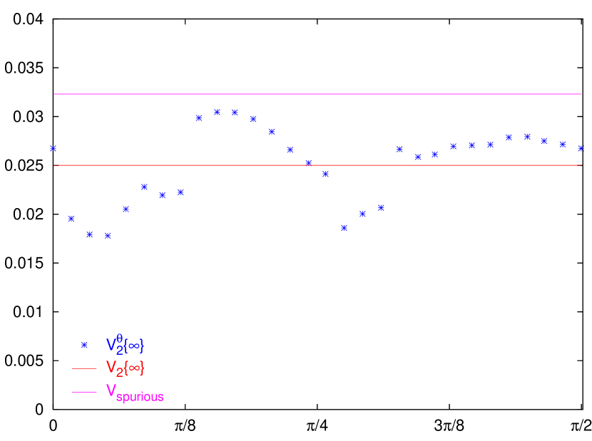
Figure 5: Analysis of $N_{\rm evts}=20000$ events of multiplicity $M=300$, simulated without anisotropic flow. Crosses show the value of the spurious flow given by our analysis, $V_{2}^{\theta}\{\infty\}/M$, as a function of $\theta$. The solid line displays the 98% CL upper bound on this spurious flow (see text).

Finally, a close look at the figure shows that the variation of $V_{2}^{\theta}\{\infty\}$ with $\theta$ has four discontinuities, which can be qualitatively understood in the following way: when $\theta$ varies, $G^{\theta}(ir)$ varies continuously, but the first minimum of $|G^{\theta}(ir)|$ may disappear for some value of $\theta$. Then, the second minimum becomes the first, and $V_{2}^{\theta}\{\infty\}$ suddenly jumps to a lower value (and vice-versa when a minimum appears below the first minimum). Such discontinuities are not expected when the minimum is due to anisotropic flow, and are by themselves a hint that the observed flow estimate is an effect of statistical fluctuations.

VII.5 Statistical error on the integrated flow

In this Section, we again assume that there is flow in the system, and that it is larger than the limit determined in the previous Section (“spurious flow”), below which the method cannot give reliable results. In that regime, we compute the statistical error on the integrated flow estimate $V_{n}^{\theta}\{\infty\}$, and on its average over directions $\theta$, due to the limited number of events. We shall in particular see that averaging several (typically 4 or 5) values of $V_{n}^{\theta}\{\infty\}$ results in a decrease in the statistical uncertainty of a factor of almost 2.

As explained in Sec. II.2, integrated flow is determined from the first minimum of $|G^{\theta}(ir)|$, which is denoted by $r_{0}^{\theta}$. According to the discussion in Sec. VII.3, for small fluctuations, this minimum is to leading order the first zero of $G_{\rm c.l.}(ir)+{\rm Re}\,\delta G^{\theta}(ir)$. It differs from $r_{0}$ [the first zero of $G_{\rm c.l.}(ir)$, given by Eq. (27)] by

$$r_{0}^{\theta}-r_{0}=-\frac{{\rm Re}\,\delta G^{\theta}(ir)}{\displaystyle\left.\frac{dG_{\rm c.l.}(ir)}{dr}\right|_{r=r_{0}}}.$$ (95)

Using Eq. (26), and replacing $r_{0}$ with its value $j_{01}/V_{n}$ [Eq. (27)], one obtains the denominator of this expression:

$$\frac{dG_{\rm c.l.}(ir)}{dr}|_{r=r_{0}}=-V_{n}\,J_{1}(j_{01})\,\exp\!\left(-\frac{j_{01}^{2}}{4\,\chi^{2}}\right),$$ (96)

where $\chi$ is the resolution parameter defined by Eq. (65). Using now Eq. (12), and reinserting Eq. (96) in Eq. (95), one deduces the statistical fluctuation of the integrated flow estimate, $\delta V_{n}^{\theta}\equiv V_{n}^{\theta}\{\infty\}-V_{n}$:

$$\frac{\delta V_{n}^{\theta}}{V_{n}} = -\frac{r_{0}^{\theta}-r_{0}}{r_{0}}$$ (97)

$$= -\frac{\exp\left(j_{01}^{2}/(4\,\chi^{2})\right)}{j_{01}J_{1}(j_{01})}\,{\rm Re}\,\delta G^{\theta}(ir_{0}).$$ (98)

The correlation $\langle\delta V_{n}^{\theta}\delta V_{n}^{\theta^{\prime}}\rangle$ can then be evaluated using Eq. (87). In this equation, the last term in the rhs vanishes since $r=r^{\prime}=r_{0}$, and $G_{\rm c.l.}(ir_{0})=0$ by definition of $r_{0}$. In order to evaluate the first and second terms in the rhs, we use the expression of the expectation value $G_{\rm c.l.}(ir)$, Eq. (26), and the two straightforward identities [see Eq. (71)]

$$|z+z^{\prime}| = 2r_{0}\cos\left(n(\theta-\theta^{\prime})/2\right)$$ (99)

$$|z-z^{\prime}| = 2r_{0}\sin\left(n(\theta-\theta^{\prime})/2\right).$$ (100)

One thus obtains

$$\frac{\left\langle\delta V_{n}^{\theta}\,\delta V_{n}^{\theta^{\prime}}\right\rangle}{V_{n}^{2}} = \frac{1}{2N_{\rm evts}\,j_{01}^{2}\,J_{1}(j_{01})^{2}}\left[\exp\!\left(\frac{j_{01}^{2}}{2\chi^{2}}\cos n(\theta-\theta^{\prime})\right)\,J_{0}\!\left(2\,j_{01}\,\sin\left(\frac{n(\theta-\theta^{\prime})}{2}\right)\right)\right.$$ (102)

$$\qquad\qquad\qquad\qquad\quad+\left.\exp\!\left(-\frac{j_{01}^{2}}{2\chi^{2}}\cos n(\theta-\theta^{\prime})\right)\,J_{0}\!\left(2\,j_{01}\,\cos\left(\frac{n(\theta-\theta^{\prime})}{2}\right)\right)\right].$$

Setting $\theta^{\prime}=\theta$, we obtain the standard deviation on $V_{n}^{\theta}\{\infty\}$ :

$$\frac{\left\langle(\delta V_{n}^{\theta})^{2}\right\rangle}{V_{n}^{2}} = \frac{1}{2N_{\rm evts}\,j_{01}^{2}\,J_{1}(j_{01})^{2}}\left[\exp\!\left(\frac{j_{01}^{2}}{2\chi^{2}}\right)+\exp\!\left(-\frac{j_{01}^{2}}{2\chi^{2}}\right)\,J_{0}\!\left(2\,j_{01}\right)\right].$$ (103)

These relations show that the relative statistical error on integrated flow depends on the parameters $V_{n}$ and $\sigma$ only through the resolution parameter $\chi$, as explained in Sec. VII.1. One sees that the error diverges exponentially for small $\chi$, while the divergence is only polynomial with finite-order cumulants Borghini:2001vi .

The linear correlation coefficient between two estimates $V_{n}^{\theta}\{\infty\}$ and $V_{n}^{\theta^{\prime}}\{\infty\}$ is defined as

$$c(\theta-\theta^{\prime})\equiv\frac{\left\langle\delta V_{n}^{\theta}\,\delta V_{n}^{\theta^{\prime}}\right\rangle}{\sqrt{\left\langle(\delta V_{n}^{\theta})^{2}\right\rangle\left\langle(\delta V_{n}^{\theta^{\prime}})^{2}\right\rangle}}.$$ (104)

It may vary between $-1$ and 1, which correspond to the cases when $\delta V_{n}^{\theta}\{\infty\}$ and $\delta V_{n}^{\theta^{\prime}}\{\infty\}$ are opposite or equal, respectively. The variation of the correlation coefficient $c(\theta-\theta^{\prime})$, computed with the help of Eqs. (102) and (103), is displayed in Fig. 6 as a function of the relative angle for several values of $\chi$. One sees that the correlation is maximum for $\theta^{\prime}=\theta$ and $\theta^{\prime}=\theta+\pi/n$, which is natural since $V_{n}^{\theta+\pi/n}=V_{n}^{\theta}$. For small values of $\chi$, the correlation vanishes when the relative angle $\theta^{\prime}-\theta$ is large enough, while for larger values of $\chi$, an anticorrelation appears around $\theta^{\prime}=\theta+\pi/2n$.

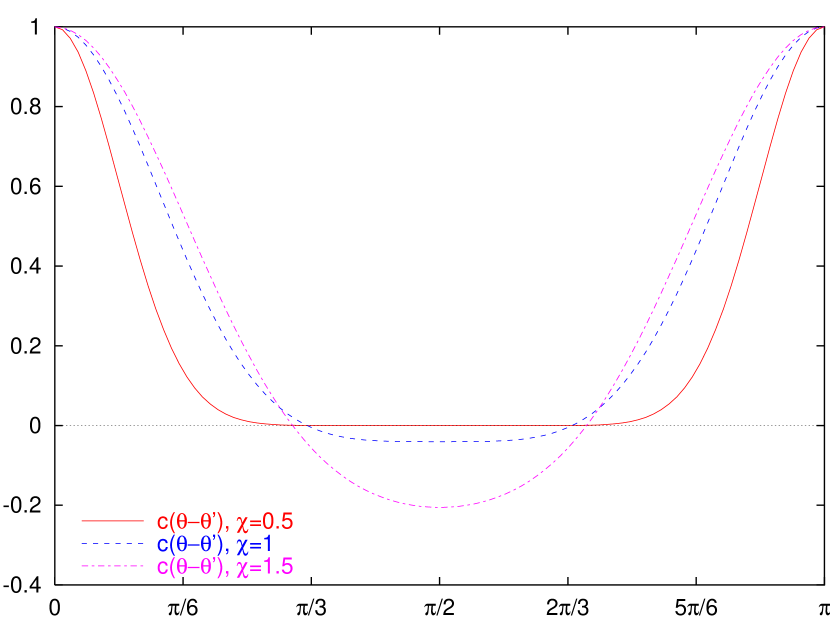
Figure 6: Correlation function $c(\theta-\theta^{\prime})$, defined by Eq. (104), as a function of $n(\theta-\theta^{\prime})$ for three values of the resolution parameter, $\chi=0.5,1,1.5$.

The shape of the correlation function $c(\theta-\theta^{\prime})$ shows that different estimates (for different values of $\theta$) are not necessarily strongly correlated. In order to decrease the statistical error, one can thus average $V^{\theta}_{n}\{\infty\}$ over several values of $\theta$. These can be chosen equally spaced, i.e., $\theta=k\pi/p$ with $k=0,\cdots,p-1$. The statistical error on this average can be derived from Eq. (102). Numerical estimates for various values of $\chi$ and different numbers of values of $\theta$ are given in Table 2, where we have assumed that $N_{\rm evts}=20000$ events have been analyzed. This Table shows two features. First, the value of the error badly diverges when the resolution parameter $\chi$ decreases, so that it is very unlikely that our method can be applied when $\chi$ is smaller than 0.5, unless a huge number of events are available, in agreement with our discussion in Sec. VII.4. Second, the statistical error decreases when the number of values of $\theta$ increases, but quickly saturates, so that in practice, 4 or 5 values of $\theta$ are enough.

Table 2: Relative statistical error on $V_{n}\{\infty\}$, for $N_{\rm evts}=20000$ events and various values of the resolution parameter $\chi$ and the number of values of $\theta$.

Nb of points	$\chi\!=\!0.6$	$\chi\!=\!0.7$	$\chi\!=\!0.8$	$\chi\!=\!1$	$\chi\!=\!1.5$
1	22.2%	7.7%	3.8%	1.70%	0.75%
2	15.7%	5.4%	2.7%	1.18%	0.46%
3	12.8%	4.4%	2.2%	0.98%	0.41%
4	11.4%	4.0%	2.1%	0.94%	0.41%
5	11.0%	3.9%	2.0%	0.94%	0.41%
$+\infty$	10.9%	3.9%	2.0%	0.94%	0.41%

The statistical error is of course minimum when the number of values of $\theta$ goes to infinity. It is then given by averaging Eq. (102) over both $\theta$ and $\theta^{\prime}$. One obtains

$$\frac{\left\langle(\delta V_{n})^{2}\right\rangle}{V_{n}^{2}}=\frac{2}{N_{\rm evts}}\frac{1}{j_{01}^{2}J_{1}(j_{01})^{2}}\sum_{q=1}^{+\infty}J_{q}(j_{01})^{2}I_{q}\!\left(\frac{j_{01}^{2}}{2\chi^{2}}\right).$$ (105)

Values in the last line of Table 2 were calculated using this expression.

It is instructive to compare the statistical error on $V_{n}\{\infty\}$ to that on estimates from cumulants of $2k$-particle correlations (where $k=1,2,\cdots$), denoted by $V_{n}\{2k\}$ in Ref. Borghini:2001vi . In both cases, the statistical error depends on two parameters, namely the total number of events, $N_{\rm evts}$, and the parameter $\chi$. However, the $\chi$-dependence of the errors is very different. Thus, whereas the statistical uncertainties on the flow estimates from cumulants for small $\chi$ diverges like a power law $1/\chi^{2k}$ (see Appendix D in Ref. Borghini:2001vi ), the error on $V_{n}\{\infty\}$ depends exponentially on $\chi$ [see Eq. (103)]. That explains why the detected multiplicity per event, which influences the value of $\chi$, plays a most crucial role in the present method, while cumulants could accommodate lower statistics.

A numerical comparison is made in Table 3 for various values of the resolution parameter $\chi$. As anticipated, for small $\chi$, the relative error on $V_{n}\{\infty\}$ is significantly larger than that on $V_{n}\{2k\}$. One also notes that the statistical error on $V_{n}\{\infty\}$ is always larger than the error on the standard flow estimate (from two-particle correlations) $V_{n}\{2\}$. For values of $\chi$ of order unity, however, the statistical error on $V_{n}\{\infty\}$ is not much larger than the error on the two-particle estimate $V_{n}\{2\}$. One must keep in mind here that lower order estimates such as $V_{n}\{2\}$ are biased by nonflow correlations, and that the resulting systematic error is usually much larger than the statistical error.

Table 3: Comparison between different methods: the relative statistical error on the integrated flow $V_{n}$ is shown for the cumulant method Borghini:2001vi , and various cumulant orders (denoted by $V_{n}\{2k\}$ with integer $k$), and for the present method ($V_{n}\{\infty\}$). As in the previous table, the number of events is $N_{\rm evts}=20000$ events, and the resolution parameter $\chi$ takes several values.

	$\chi\!=\!0.6$	$\chi\!=\!0.7$	$\chi\!=\!0.8$	$\chi\!=\!1$	$\chi\!=\!1.5$
$\delta V_{n}\{2\}/V_{n}$	1.3%	1.0%	0.83%	0.62%	0.37%
$\delta V_{n}\{4\}/V_{n}$	4.5%	2.7%	1.8%	1.00%	0.43%
$\delta V_{n}\{6\}/V_{n}$	7.7%	3.7%	2.1%	0.99%	0.41%
$\delta V_{n}\{8\}/V_{n}$	9.9%	4.1%	2.1%	0.95%	0.41%
$\delta V_{n}\{\infty\}/V_{n}$	10.9%	3.9%	2.0%	0.94%	0.41%

One also sees clearly in Table 3 that the error on the present estimate $V_{n}\{\infty\}$ is the limit of the error on $V_{n}\{2k\}$ as $k$ goes to infinity, for fixed $\chi$. This reflects the fact that $V_{n}\{\infty\}$ is itself the limit of $V_{n}\{2k\}$ as $k$ goes to infinity, as explained in Sec. III. It is interesting to note that the statistical error does not increase monotonically with the order of the cumulant $2k$, as one might think. This was already pointed out in Ref. Borghini:2001vi . For a fixed $\chi$, the error on $V_{n}\{2k\}$ first increases as $k$ increases, reaches a maximum for some value of $k$ and then slightly decreases. This can be seen in the last four columns of Table 3. While the statistical error is always smallest for the standard, two-particle estimate $V_{n}\{2\}$, the error on $V_{n}\{\infty\}$ is smaller than that on the estimate from four-particle correlations $V_{n}\{4\}$ as soon as $\chi$ exceeds $0.89$. Comparing with the values of $\chi$ given in Table 1, this suggests that the new method can be used without problem at RHIC. The statistical error on our flow estimate is expected to be comparable to that on the estimate from four-particle cumulants, and significantly smaller than the systematic error (due to nonflow correlations) on the estimate from the standard method Adler:2002pu .

VII.6 Statistical error on the differential flow

We now turn to the statistical uncertainty on the differential flow estimates $v^{\prime\theta}_{mn}$ and its average over $\theta$, $v^{\prime}_{mn}$. Note that, unlike the case of integrated flow, the errors we shall compute in this Section are absolute errors, not relative ones.

Since differential flow is analyzed in principle in a narrow phase-space window, the statistical error on differential flow is much larger than the error on integrated flow. We therefore neglect the statistical error on integrated flow here: in Eq. (15), we replace $V_{n}\{\infty\}$ and $r_{0}^{\theta}$ by their theoretical values, i.e., $V_{n}$ and $r_{0}$ [see Eq. (27)]. Similarly, we replace in the denominator the sample average by an expectation value:

$$\left\{Q^{\theta}e^{ir_{0}^{\theta}Q^{\theta}}\right\} \simeq \left\langle Q^{\theta}e^{ir_{0}Q^{\theta}}\right\rangle$$ (106)

$$= -i\,\frac{dG_{\rm c.l.}(ir)}{dr}|_{r=r_{0}},$$ (107)

where the rhs is given by Eq. (96). Equation (15) then becomes

$$v^{\prime\theta}_{mn}\{\infty\}\equiv(-1)^{m}\,\frac{e^{j_{01}^{2}/(4\chi^{2})}}{J_{m}(j_{01})}\,\left\{\cos\left(mn(\psi-\theta)\right)\,{\rm Re}\left(i^{m}G(r_{0}^{\theta}\,e^{i\theta})\right)\right\}.$$ (108)

We now evaluate the correlation between $v^{\prime\theta}_{mn}\{\infty\}$ and $v^{\prime\theta^{\prime}}_{mn}\{\infty\}$, using an equation similar to Eq. (79), with $N_{\rm evts}$ replaced by the total number of “differential particles”, $N^{\prime}$. We assume, for simplicity, that $\psi$ and $G(z)$ are statistically independent (which means in particular that the differential flow vanishes) so that the term involving $\psi$ factors out. Averaging over $\psi$, this term gives

$$\left\langle\cos(mn(\psi-\theta))\cos(mn(\psi-\theta^{\prime}))\right\rangle=\frac{1}{2}\cos(mn(\theta-\theta^{\prime})).$$ (109)

One thus obtains

$$\left\langle\delta v_{mn}^{\prime\theta}\{\infty\}\,\delta v_{mn}^{\prime\theta^{\prime}}\{\infty\}\right\rangle=\frac{\cos(mn(\theta-\theta^{\prime}))\,e^{j_{01}^{2}/(2\chi^{2})}}{2N^{\prime}\,J_{m}(j_{01})^{2}}\left\langle{\rm Re}\,(i^{m}e^{ir_{0}Q^{\theta}})\,{\rm Re}\,(i^{m}e^{ir_{0}Q^{\theta^{\prime}}})\right\rangle.$$ (110)

Now, ${\rm Re}\,(i^{m}G(z))$ is, up to a sign, the real (resp. imaginary) part of $G(z)$ for even (resp. odd) $m$. Using Eq. (76) and Eq. (26), one finally obtains

$$\left\langle\delta v_{mn}^{\prime\theta}\{\infty\}\,\delta v_{mn}^{\prime\theta^{\prime}}\{\infty\}\right\rangle = \frac{\cos(mn(\theta-\theta^{\prime}))}{4N^{\prime}\,J_{m}(j_{01})^{2}}\left[\exp\!\left(\frac{j_{01}^{2}}{2\chi^{2}}\cos\left(n(\theta-\theta^{\prime})\right)\right)\,J_{0}\!\left(2j_{01}\,\sin\!\left(\frac{n(\theta-\theta^{\prime})}{2}\right)\right)\right.$$ (112)

$$\qquad\qquad\qquad\qquad+\ (-1)^{m}\left.\exp\!\left(-\frac{j_{01}^{2}}{2\chi^{2}}\cos n(\theta-\theta^{\prime})\right)\,J_{0}\!\left(2j_{01}\,\cos\!\left(\frac{n(\theta-\theta^{\prime})}{2}\right)\right)\right],\qquad$$

where $N^{\prime}$ is the number of particles in the considered phase-space bin. One checks that this expression is invariant under the transformation $\theta\to\theta+\pi/n$, as expected from the symmetry property $v_{mn}^{\prime\theta}\{\infty\}=v_{mn}^{\prime\theta+\pi/n}\{\infty\}$. Setting $\theta=\theta^{\prime}$ in Eq. (112) yields the absolute statistical error on $v_{mn}^{\prime\theta}$.

As in the case of integrated flow, one must average over several values of $\theta$ in order to reduce the statistical error. Tables 4 and 5 show the variation of the error as the number of values of $\theta$ increases, for the first two harmonics $v^{\prime}_{n}\{\infty\}$ and $v^{\prime}_{2n}\{\infty\}$. Once again, 4 or 5 values of $\theta$ are enough in practice to minimize the statistical error. In the limit when the number of $\theta$ goes to infinity, the error is given by

$$\left\langle v^{\prime}_{mn}\{\infty\}^{2}\right\rangle-(v^{\prime}_{mn})^{2}=\hskip 170.71652pt$$ (114)

$$\frac{1}{2\,N^{\prime}\,J_{m}(j_{01})^{2}}\sum_{q=-\infty}^{+\infty}J_{q}(j_{01})^{2}I_{q+m}\!\left(\frac{j_{01}^{2}}{2\chi^{2}}\right).$$

Table 4: Statistical error on the reconstructed value of the differential flow $v^{\prime}_{n}$, for $N^{\prime}=6\times 10^{5}$ particles in the bin, and various values of the resolution parameter and the number of values of $\theta$. Note that these are absolute values, not relative values as in Tables 2 and 3.

Nb of points	$\chi=0.6$	$\chi=0.7$	$\chi=0.8$	$\chi=1$	$\chi=1.5$
1	6.9%	2.4%	1.19%	0.53%	0.24%
2	4.9%	1.7%	0.84%	0.37%	0.17%
3	4.0%	1.4%	0.69%	0.31%	0.14%
4	3.5%	1.2%	0.63%	0.29%	0.14%
5	3.4%	1.2%	0.62%	0.29%	0.14%
$+\infty$	3.3%	1.2%	0.62%	0.29%	0.14%

Table 5: Same as Table 4, but for the higher harmonic $v^{\prime}_{2n}$.

Nb of points	$\chi=0.6$	$\chi=0.7$	$\chi=0.8$	$\chi=1$	$\chi=1.5$
1	8.3%	2.9%	1.43%	0.63%	0.28%
2	5.9%	2.0%	1.02%	0.46%	0.22%
3	4.8%	1.7%	0.83%	0.37%	0.17%
4	4.1%	1.4%	0.72%	0.32%	0.15%
5	3.8%	1.3%	0.69%	0.32%	0.15%
$+\infty$	3.7%	1.3%	0.68%	0.32%	0.15%

It is also interesting to compare the error computed in this Section with the statistical errors on differential flow estimates from multiparticle cumulants Borghini:2001vi . This comparison is performed in Tables 6 and 7 for the first two harmonics $v^{\prime}_{n}$ and $v^{\prime}_{2n}$, respectively. The same comments apply here as for the integrated flow (Sec. VII.5): statistical errors on $v^{\prime}_{mn}\{\infty\}$ are much larger than errors on standard flow estimates for small $\chi$, but become comparable, and even smaller than estimates from higher-order cumulants, when $\chi$ is close to unity or larger.

Table 6: Comparison between different methods: the statistical error on the differential flow $v^{\prime}_{n}$ is shown for the estimates from cumulant of 2-particle ($v^{\prime}_{n}\{2\}$) and 4-particle ($v^{\prime}_{n}\{4\}$) correlations Borghini:2001vi and for the present method ($v^{\prime}_{n}\{\infty\}$). As in the previous table, we assume $N^{\prime}=6\times 10^{5}$ particles in the bin, the resolution parameter $\chi$ takes several values.

	$\chi=0.6$	$\chi=0.7$	$\chi=0.8$	$\chi=1$	$\chi=1.5$
$\delta v^{\prime}_{n}\{2\}$	0.18%	0.16%	0.15%	0.13%	0.11%
$\delta v^{\prime}_{n}\{4\}$	0.88%	0.61%	0.45%	0.29%	0.15%
$\delta v^{\prime}_{n}\{\infty\}$	3.3%	1.2%	0.62%	0.29%	0.14%

Table 7: Same as Table 7, but for the higher harmonic $v^{\prime}_{2n}$. Errors on estimates from 3- and 5-particle cumulants Borghini:2001vi are compared with the present estimate $v^{\prime}_{2n}\{\infty\}$.

	$\chi=0.6$	$\chi=0.7$	$\chi=0.8$	$\chi=1$	$\chi=1.5$
$\delta v^{\prime}_{2n}\{3\}$	0.48%	0.38%	0.32%	0.24%	0.16%
$\delta v^{\prime}_{2n}\{5\}$	1.42%	0.88%	0.59%	0.33%	0.16%
$\delta v^{\prime}_{2n}\{\infty\}$	3.7%	1.3%	0.68%	0.32%	0.15%

In addition, one notes that the error on the higher harmonic $v^{\prime}_{2n}$ is only slightly larger than the error on $v^{\prime}_{n}$, while in standard flow analyses the error on higher harmonics is often much larger. It turns out that in the case of higher harmonics, the statistical error on $v^{\prime}_{mn}\{\infty\}$ is even smaller than the statistical error on the estimate from the standard flow analysis [which we denote by $v^{\prime}_{mn}\{m+1\}$ since it involves a ($m+1$)-particle correlation], if the resolution parameter $\chi$ is large enough. More precisely, our method yields smaller error bars than the standard method as soon as $\chi>1.3$ for $v^{\prime}_{2n}$, $\chi>1.1$ for $v^{\prime}_{3n}$, and $\chi>0.94$ for $v^{\prime}_{4n}$. Even from the point of view of statistical error bars, it seems to be the best method to measure higher harmonics $v_{3}$, $v_{4}$, or at least to set upper bounds on their values, which could easily be done at SIS or AGS energies where the reaction plane resolution is high: correlating more particles may in some cases lead to smaller statistical fluctuations, which is a rather unexpected conclusion. However, one must keep in mind that systematic errors on these higher harmonics may be large, as shown in Sec. V.2.

VIII Detector effects

Until now, we have performed all calculations assuming that the detector is perfect, in the sense that it is azimuthally isotropic. In this Section, we shall relax this assumption, and investigate the influence of acceptance inefficiencies on the determination of flow through the present method. As we shall see, the generating function will acquire a phase, which does not affect the fact that the zeroes lie on the imaginary axis. The only sizeable effect on the $\theta$-averaged estimate $V_{n}\{\infty\}$ is of second order in the acceptance coefficients $a_{n}$ which we soon define, and is negligible in most practical cases.

Let us denote by $A(\phi)$ the probability that a particle with azimuthal angle $\phi$ be detected: $A(\phi)$ represents the acceptance-efficiency profile of the detector. We choose the normalization $\int_{0}^{2\pi}\!A(\phi)\,d\phi/2\pi=1$. We assume for simplicity that $A(\phi)$ is independent of the rapidity and transverse momentum of the particle. Since $A(\phi)$ is a $2\pi$-periodic function, it is natural to expand it in Fourier series. We denote by $a_{p}$ the corresponding Fourier coefficients:

$$a_{n}\equiv\int_{0}^{2\pi}\!e^{-in\phi}A(\phi)\,\frac{d\phi}{2\pi}.$$ (115)

The normalization choice of course reads $a_{0}=1$.

The probability distribution of $\phi$ for particles seen in the detector, for a fixed orientation of the reaction plane $\Phi_{R}$, is then

$$\frac{dN}{d\phi}=A(\phi)\sum_{n=-\infty}^{+\infty}v_{n}e^{in(\phi-\Phi_{R})},$$ (116)

where we use the conventions $v_{-n}\equiv v_{n}$, $v_{0}\equiv 1$.

Using this distribution, we can compute the generating function as in Sec. III.3. Equation (20) still holds, but $\left\langle Q^{\theta}|\Phi_{R}\right\rangle$ is no longer given by Eq. (21), which holds only with a perfect acceptance. From the definition of $Q^{\theta}$, Eq. (4), we obtain instead

$$\left\langle Q^{\theta}|\Phi_{R}\right\rangle=\sum_{m=-\infty}^{+\infty}V_{m}\,{\rm Re}\left(a_{n-m}e^{in\theta}e^{-im\Phi_{R}}\right),$$ (117)

which replaces Eq. (21) for an arbitrary detector. For a perfect acceptance ($a_{0}=1$, $a_{n\neq 0}=0$), this expression reduces to Eq. (21), as should be.

We shall now assume for simplicity that only one Fourier harmonic of the flow, $v_{n}$, is non-vanishing, with $n\neq 0$. This is most probably a reasonable assumption at ultrarelativistic energies. Then, only three terms contribute in the sum, $m=-n$, $m=0$ and $m=n$. We may then rewrite the previous equation as

$$\left\langle Q^{\theta}|\Phi_{R}\right\rangle = V_{0}\,{\rm Re}\left(a_{n}e^{in\theta}\right)$$ (119)

$$+\ V_{n}\,{\rm Re}\!\left[\left(1+a_{2n}e^{2in\theta}\right)\,e^{in(\Phi_{R}-\theta)}\right],\qquad$$

where $V_{0}=\langle\sum w_{j}\rangle$ and we have used the normalization condition $a_{0}=1$, as well as the properties $a_{-2n}=a_{2n}^{*}$, see Eq. (115), and $V_{-n}=V_{n}$, which follows from Eqs. (2) and (6). Inserting this value in Eq. (20), we obtain

$$\left\langle e^{zQ^{\theta}}|\Phi_{R}\right\rangle=\exp\left(z\,V_{0}\,{\rm Re}\left(a_{n}e^{in\theta}\right)+\frac{\sigma^{2}z^{2}}{4}+z\,V_{n}\,{\rm Re}\!\left[\left(1+a_{2n}e^{2in\theta}\right)e^{in(\Phi_{R}-\theta)}\right]\right).$$ (120)

Averaging this expression over $\Phi_{R}$ (we still assume that $\sigma$ is independent of $\Phi_{R}$), we obtain

$$G^{\theta}(z)=e^{z\,V_{0}\,{\rm Re}(a_{n}e^{in\theta})+\sigma^{2}z^{2}/4}\,I_{0}\!\left(z\,V_{n}\left|1+a_{2n}e^{2in\theta}\right|\right).$$ (121)

Comparing this result with the perfect-acceptance case in Eq. (25), there appear several modifications. First of all, $G^{\theta}(z)$ is no longer real-valued for values of $z$ on the imaginary axis. Then, there is a new term in the exponential factor, which involves the acceptance coefficient $a_{n}$. This term cannot produce any spurious zero of $G^{\theta}(z)$, nor shift the position of the zeroes. When $z$ is purely imaginary, it is a pure phase, which goes away when taking the modulus $|G^{\theta}(z)|$. However, this phase makes the real part of $G^{\theta}(z)$ oscillate, and thus makes it vanish on the imaginary axis. This explains why it was important to consider (the minimum of) the modulus, not (the zero of) the real part, as mentioned in Sec. III.3.

The remaining modification is more relevant for the procedure introduced in Sec. II.2, since it results in a shifting of the position of the generating-function zeroes. The argument of the Bessel function in Eq. (121) now depends on $\theta$, and involves the acceptance coefficient $a_{2n}$. Thus, using Eq. (12), we now obtain

$$V_{n}^{\theta}\{\infty\}=V_{n}\left|1+a_{2n}e^{2in\theta}\right|,$$ (122)

where $a_{2n}$ is given by Eq. (115): the estimate $V_{n}^{\theta}$ now depends on $\theta$, as can be seen in Fig. 4. As expected from the general discussion in Sec. II.2, it is ($\pi/n$)-periodic. In the case of a detector with a hole of $\alpha$ radians around $\phi=\pi$, an explicit calculation gives $a_{2n}=-\sin(n\alpha)/[(2\pi-\alpha)n]$. Thus, in the simulation of Sec. II.4, $a_{4}\simeq 0.0827$, quite a small number, but large enough to yield the $\theta$-dependence observed in Fig. 4.

Averaging Eq. (122) over $\theta$, one obtains

$$V_{n}\{\infty\}=V_{n}(1+|a_{2n}|^{2}).$$ (123)

The relative error is $|a_{2n}|^{2}$, which is in practice small if the detector has a reasonable azimuthal coverage.

Consider now differential flow. We leave open the possibility that the corresponding acceptance function is not the same as for integrated flow, and we denote by $a^{\prime}_{n}$ the Fourier acceptance coefficients for the differential particle. For the sake of brevity, we shall only consider the case $m=1$ (differential flow in the same harmonic as integrated flow); the generalization to $m$ arbitrary only involves much more tedious calculations. Finally, we make the same assumption as above, namely, that only one flow harmonic does not vanish.

Under this assumption, Eq. (39) is replaced with an equation similar to Eq. (119)

$$\left\langle\cos(n(\psi-\theta))|\Phi_{R}\right\rangle=v^{\prime}_{n}\,{\rm Re}\left[(1+a^{\prime}_{2n}e^{2in\theta})e^{in(\Phi_{R}-\theta)}\right].$$ (124)

This identity can be then combined with Eq. (120) to compute $D_{m}^{\theta}(z)$ defined by Eq. (33). To perform the integration over $\Phi_{R}$, one can use the following integral:

$$\int_{0}^{2\pi}\!{\rm Re}\left(Be^{im\varphi}\right)e^{z\,{\rm Re}(Ae^{i\varphi})}\,\frac{d\varphi}{2\pi}=\frac{{\rm Re}(B\,{A^{*}}^{m})}{|A|^{m}}\,I_{m}(z|A|),$$ (125)

valid for arbitrary complex numbers $A$ and $B$. We use this result with $m=1$ (other values of $m$ might be useful for higher harmonics) and $\varphi=\Phi_{R}-\theta$:

$$D_{1}^{\theta}(z)=e^{z\,V_{0}\,{\rm Re}(a_{n}e^{in\theta})+\sigma^{2}z^{2}/4}\,\frac{{\rm Re}\left[(1+a^{\prime}_{2n}e^{2in\theta})(1+a_{2n}^{*}e^{-2in\theta})\right]}{\left|1+a_{2n}e^{2in\theta}\right|}\,I_{1}\!\left(zV_{n}\left|1+a_{2n}e^{2in\theta}\right|\right)\,v^{\prime}_{n}.$$ (126)

Note that the exponential prefactor and the argument of the Bessel function are the same as in Eq. (121). After some algebra, similar to that in Sec. III.5, one finally obtains

$$v^{\prime\theta}_{n}\{\infty\}=v^{\prime}_{n}\,\frac{{\rm Re}\left[(1+a^{\prime}_{2n}e^{2in\theta})(1+a_{2n}^{*}e^{-2in\theta})\right]}{\left|1+a_{2n}e^{2in\theta}\right|}.$$ (127)

As in the case of integrated flow, acceptance inefficiencies result in the appearance of a $\theta$-dependent, ($\pi/n$)-periodic, multiplicative coefficient in front of $v^{\prime}_{n}$. In the particular case where $a^{\prime}_{2n}=a_{2n}$, Eq. (127) gives

$$v^{\prime\theta}_{n}\{\infty\}=v^{\prime}_{n}\left|1+a_{2n}e^{2in\theta}\right|.$$ (128)

Integrating over phase space, one recovers Eq. (122).

IX Concluding remarks

In this paper, we have introduced a new method of analysis of anisotropic flow in heavy-ion collisions. This is the first method to extract both integrated and differential flow from the interparticle correlations between a large number of particles, rather than from the correlations between only a small number. Thus, it is able to isolate a collective effect which involves all particles, such as flow, removing the influence of other, “nonflow” effects, which can bias few-particle methods. The flow estimates obtained with the new method are therefore more reliable than with any other method.

This increased reliability is of course important inasmuch as flow is concerned: with more accurate collective flow estimates, the constraints on models become stronger. But it also matters for the measurement of other effects, as for instance when reconstructing jets from the azimuthal correlations they induce between high momentum particles at ultrarelativistic energies Adler:2002ct ; Adler:2002tq ; Agakichiev:2003gg . At high $p_{T}$, (elliptic) flow is large, and constitutes a huge background. It is most important to know its magnitude accurately to extract nonflow correlations.

Let us enter into a little more detail. The method relies on the search of the first minimum of a generating function of multiparticle azimuthal correlations; the actual position of this minimum directly yields an integrated flow estimate. Once the minimum has been found, computing a second function at its position gives differential flow. This procedure is simpler to implement than other methods of flow analysis. It is significantly faster numerically, and less tedious, than the methods based on cumulants of multiparticle correlations. In addition, in the differential flow analysis there is no need to subtract autocorrelations, which are negligible. Finally, detector effects are negligible as well in most cases. We have carefully studied the various sources of errors, either systematic errors intrinsic to the method (due to nonflow effects, higher flow harmonics, detector inefficiencies), or statistical errors. This allows us to conclude that it is the most accurate method to measure both directed and elliptic flow in collisions from 100 MeV to a few GeV per nucleon (SIS and AGS energies) and elliptic flow at ultrarelativistic energies, especially at RHIC and the CERN Large Hadron Collider (LHC).

It may be possible to extend the method, so as to be able to measure directed flow at ultrarelativistic energies as well, paralleling the step which led from the cumulant method of Refs. Borghini:2000sa ; Borghini:2001vi to that of Ref. Borghini:2002vp . Namely, the generating function of one complex variable $G(z)$ could be generalized to a two-variable function $G(z_{1},z_{2})$ involving azimuthal correlations in two different harmonics (corresponding to $v_{1}$ and $v_{2}$) at once. This new function could then be used to measure directed flow using as a reference the elliptic flow, which is large at ultrarelativistic energies, and thus provides a good reference.

Another generalization of the method would be to extract directly nonflow azimuthal correlations, and especially, to obtain them with respect to the impact-parameter direction in non-central collisions. This could be done, for instance, to study the azimuthal dependence of Hanbury–Brown Twiss (HBT) correlations Lisa:2000xj , or that of jet quenching Adler:2002tq .

Finally, thanks to the generality of its formalism, this method could easily be extended to other types of observables where “fluctuations” are of interest. It seems to be the most natural method to look for critical, large scale fluctuations in a system, which are expected in the vicinity of a phase transition Stephanov:1999zu .

Appendix A An alternative form of the generating function

The generating function on which our method is based, $G^{\theta}(z)$, has been defined in Eqs. (4) and (9):

$$G^{\theta}(z)=\left\{\exp\!\left(z\sum_{j=1}^{M}w_{j}\cos(n(\phi_{j}-\theta))\right)\right\}.$$ (129)

An alternative choice is:

$$\tilde{G}^{\theta}(z)=\left\{\prod_{j=1}^{M}\left[1+zw_{j}\cos(n(\phi_{j}-\theta))\right]\right\}.$$ (130)

The procedure to determine the integrated flow with $\tilde{G}^{\theta}(z)$ is exactly the same as for $G^{\theta}(z)$, as presented in Sec. II.2. In order to determine the differential flow, one should replace $e^{ir_{0}^{\theta}Q^{\theta}}$ in the numerator of the rhs of Eq. (15) with the term in curly brackets in the rhs of Eq. (130), with $z=ir_{0}^{\theta}$; next, one should replace $\left\{Q^{\theta}e^{ir_{0}^{\theta}Q^{\theta}}\right\}$ in the denominator of the rhs of Eq. (15) with the derivative $d\tilde{G}^{\theta}/dz$, evaluated at $z=ir_{0}^{\theta}$.

The essential point is that $\tilde{G}^{\theta}(z)$ factorizes for independent subsystems, as does $G^{\theta}(z)$, so that the discussion in Secs. III.2 and III.3 can be readily extended to $\tilde{G}^{\theta}(z)$. The only difference is that $\sigma$ in Eq. (20) is no longer given by Eq. (22). In fact, $\sigma$ vanishes for independent particles, and is generally smaller for $\tilde{G}^{\theta}$ than for $G^{\theta}$. Although the value of the generating function is modified, the zeroes remain at the same position, and in particular the first one, from which flow (either integrated or differential) is determined. A similar equivalence is also known in statistical mechanics nienhuis .

A generating function similar to $\tilde{G}^{\theta}(z)$ was chosen in the cumulant expansion of Ref. Borghini:2001vi . The argument was that when expanding in powers of $z$, $\tilde{G}^{\theta}(z)$ involves only correlations between different particles, while $G^{\theta}(z)$ involves “autocorrelation” terms. The bias induced by these autocorrelations was studied in detail in Ref. Borghini:2000sa for finite-order cumulants. In general, this bias is of the same order of magnitude as the bias induced by nonflow correlations, as explained in Sec. III.5.4.

Let us illustrate this by a simple explicit example. We repeat the calculations of Sec. IV with $\tilde{G}^{\theta}(z)$ instead of $G^{\theta}(z)$: particles are emitted in collinear jets containing $q$ particles each. If the jet angles are randomly distributed, one obtains

$$\tilde{G}^{\theta}(z)=\left\langle(1+z\cos\phi)^{q}\right\rangle^{M/q},$$ (131)

where angular brackets denote an average over $\phi$, which gives:

$$\tilde{G}^{\theta}(z)=\left(\sum_{l=0}^{[q/2]}\frac{z^{2l}}{(q-2l)!\,(l!)^{2}\,2^{2l}}\right)^{M/q}.$$ (132)

For independent particles ($q=1$) $\tilde{G}^{\theta}(z)=1$ [compare with Eq. (47)]. This function has no zero, hence the analysis yields no spurious flow. This shows that $\tilde{G}^{\theta}(z)$ is an improvement over $G^{\theta}(z)$ when there is no nonflow correlation. For higher values of $q$, $\tilde{G}^{\theta}(z)$ is a polynomial whose roots can be computed numerically. The estimate $V_{n}\{\infty\}$ is then given by Eq. (12). One obtains the values $1.70$, $2.94$, $4.07$ for $q=2,3,4$ respectively. This is very close to the value $V_{n}\{\infty\}=q$ obtained with $G^{\theta}(z)$ [see Eq. (49)], which shows that $\tilde{G}^{\theta}(z)$ no longer represents an improvement over $G^{\theta}(z)$ when nonflow correlations are present.

The same conclusions hold for systematic errors, whose order of magnitude is not modified by autocorrelations. In practice, the latter may increase the contribution of each term in the rhs of Eq. (52), but this equation remains valid as an order of magnitude, with either form of the generating function.

The final results of Secs. V to VIII also apply when $\tilde{G}^{\theta}(z)$ is used instead of $G^{\theta}(z)$, although intermediate calculations may differ. In particular, a derivation of statistical errors with a generating function similar to $\tilde{G}^{\theta}(z)$ is given in Appendix D of Borghini:2001vi .

As a conclusion, $\tilde{G}^{\theta}(z)$ is expected to give more accurate results than $G^{\theta}(z)$ when nonflow correlations are weak. The price to pay is that $\tilde{G}^{\theta}(z)$ requires much more computer time: for each value of $z$, one needs to evaluate the product over all particles in Eq. (130), instead of calculating only one flow vector, valid for all values of $z$. Furthermore, since the motivation of this paper was to obtain a method which remains valid when nonflow correlations are present, and since $\tilde{G}^{\theta}(z)$ is not better than $G^{\theta}(z)$ in this respect, we chose to use $G^{\theta}(z)$ in the paper.

Appendix B Relation with the cumulant expansion of Ref. Borghini:2000sa

In Ref. Borghini:2000sa , integrated flow was determined from the following generating function (Eq. (B2) of Ref. Borghini:2000sa ):

$$G(z_{1},z_{2})=\left\{e^{z_{1}Q+z_{2}Q^{*}}\right\},$$ (133)

where $z_{1}$ and $z_{2}$ are two independent complex variables, $Q\equiv Q_{x}+iQ_{y}$, and $Q^{*}=Q_{x}-iQ_{y}$. Cumulants $\left\langle\!\left\langle Q^{k}(Q^{*})^{l}\right\rangle\!\right\rangle$ were then defined by the power-series expansion of $\ln G(z_{1},z_{2})$:

$$\ln G(z_{1},z_{2})=\sum_{k,l}\frac{z_{1}^{k}z_{2}^{l}}{k!\,l!}\left\langle\!\left\langle Q^{k}(Q^{*})^{l}\right\rangle\!\right\rangle.$$ (134)

The new generating function, Eq. (9), can be expressed in terms of $G(z_{1},z_{2})$:

$$G^{\theta}(z)=G\!\left(\frac{ze^{-i\theta}}{2},\frac{ze^{i\theta}}{2}\right).$$ (135)

The cumulant $\left\langle\!\left\langle(Q^{\theta})^{k}\right\rangle\!\right\rangle$ defined by Eq. (18) is a linear combination of the $\left\langle\!\left\langle Q^{k-l}(Q^{*})^{l}\right\rangle\!\right\rangle$:

$$\left\langle\!\left\langle(Q^{\theta})^{k}\right\rangle\!\right\rangle=\frac{1}{2^{k}}\sum_{l=0}^{k}\left(\!\begin{array}[]{c}k\\ l\end{array}\!\right)e^{i(2l-k)\theta}\left\langle\!\left\langle Q^{k-l}(Q^{*})^{l}\right\rangle\!\right\rangle.$$ (136)

In Ref. Borghini:2000sa , the recommended procedure was to extract an estimate of the flow, denoted by $V_{n}\{2k\}$ in Ref. Borghini:2001vi , using the “diagonal” cumulants $\left\langle\!\left\langle Q^{k}(Q^{*})^{k}\right\rangle\!\right\rangle$, which are the only non-vanishing cumulants except for statistical fluctuations and detector asymmetries. By definition of the estimates, $\left\langle\!\left\langle Q^{k}(Q^{*})^{k}\right\rangle\!\right\rangle$ is equal to $(V_{n}\{2k\})^{2k}$, up to a multiplicative factor.

In the present paper, we obtain an estimate $V_{n}$ from $\left\langle\!\left\langle(Q^{\theta})^{2k}\right\rangle\!\right\rangle$, which was denoted by $V_{n}^{\theta}\{2k\}$ in Sec. III.3: By definition, $\left\langle\!\left\langle(Q^{\theta})^{2k}\right\rangle\!\right\rangle$ is equal to $(V_{n}^{\theta}\{2k\})^{2k}$, up to a multiplicative factor. In order to obtain the relation between $V_{n}^{\theta}\{2k\}$ and $V_{n}\{2k\}$, let us average Eq. (136) over $\theta$:

$$\int_{0}^{2\pi}\frac{d\theta}{2\pi}\left\langle\!\left\langle(Q^{\theta})^{2k}\right\rangle\!\right\rangle=\frac{(2k)!}{2^{2k}(k!)^{2}}\left\langle\!\left\langle Q^{k}(Q^{*})^{k}\right\rangle\!\right\rangle.$$ (137)

One then obtains the following relation:

$$\int_{0}^{2\pi}\frac{d\theta}{2\pi}(V_{n}^{\theta}\{2k\})^{2k}=(V_{n}\{2k\})^{2k}.$$ (138)

In the limit of an infinite number of events, and with a perfectly symmetric detector $V_{n}^{\theta}\{2k\}$ is independent of $\theta$ by azimuthal symmetry. The above equation shows that $V_{n}^{\theta}\{2k\}$ then coincides exactly with the estimate $V_{n}\{2k\}$. In this case, our estimate $V_{n}\{\infty\}$ is exactly the large-order limit of $V_{n}\{2k\}$ for large $k$.

However, this is no longer the case when statistical fluctuations and detector asymmetries are taken into account. In this paper, we first let the order $k$ go to infinity for a fixed value of $\theta$, and obtain the limit $V_{n}^{\theta}\{\infty\}$. Then, we average over $\theta$. On the other hand, in the method of Ref. Borghini:2000sa , one first averages over $\theta$ for a fixed $k$, which is natural when working at a finite cumulant order.

This is actually a minor difference. The only practical consequence is that acceptance corrections, which must be applied when the detector has limited azimuthal coverage, differ. The present approach, where the whole analysis is done for a fixed value of $\theta$, is more natural and leads to simpler acceptance corrections (see Sec. VIII) than the earlier method (for which the acceptance corrections were derived in Appendix C of Ref. Borghini:2001vi ).

Another difference with the method of Borghini:2000sa is that, in the latter, weights $w_{j}$ in Eq. (2) were chosen proportional to $1/\sqrt{M}$, while they are independent of $M$ in the present paper. The rationale was that lower-order cumulants contain large trivial contributions from “autocorrelations”: for instance, $\left\langle|Q^{2}|\right\rangle$ is nonvanishing even if there is no flow. With the chosen weight, these contributions were independent of $M$ and could easily be subtracted. However, the magnitude of these autocorrelations becomes smaller and smaller as the cumulant order increases, and they are negligible with the present method (which is the limit of asymptotically large order), so that $1/\sqrt{M}$ factors are no longer required.

In Ref. Borghini:2001vi , an improvement over the method of Ref. Borghini:2000sa was proposed, using a generating function similar to $\tilde{G}^{\theta}(z)$ in Eq. (130). This new formulation was free from autocorrelations. However, we pointed out that when the detector has limited azimuthal coverage, multiplicity fluctuations induce errors on lower-order cumulants which are similar to the errors induced by autocorrelations. These errors were minimized by taking weights proportional to $1/M$, and using a slightly modified definition of the generating function of cumulants (Eq. (7) of Ref. Borghini:2001vi ). With the present method, such a refinement is not necessary.

In this paper, we choose to work with weights which are independent of $M$ for two reasons: first, this simplifies the discussion of Sec. III and makes the relation to Lee-Yang theory clearer. Second, the multiplicity may not be a relevant quantity in heavy-ion experiments at lower energies, where a nuclear fragment contributes as much to the flow as several nucleons. However, our analysis could as well be performed with $M$-dependent weights. The only difference is that the integrated flow $V_{n}$ would scale differently with the multiplicity, and its fluctuations with impact parameter, studied in Sec. VI, would also differ.

Appendix C Large orders

Consider a function $f(z)$ which is analytic in the vicinity of the origin. It can be expanded in power series:

$$f(z)=\sum_{k=0}^{\infty}a_{k}z^{k}.$$ (139)

The coefficients $a_{k}$ can be expressed in integral form:

$$a_{k}=\oint\frac{f(z)}{z^{k+1}}\frac{dz}{2i\pi},$$ (140)

where the integration contour circles the origin in the complex plane (full line in Fig. 7). The integration contour can then be expanded until it reaches a singularity of $f(z)$ (see Fig. 7). We are interested in the asymptotic behavior of the coefficients $a_{k}$ as $k$ goes to infinity. For large $k$, the integral in Eq. (140) is dominated by the smallest values of $|z|$. Therefore, the large-order behavior of $a_{k}$ is determined by the singularities of $f(z)$ which are closest to the origin.

The first case of interest in this paper (Sec. III.2) is $f(z)=\ln G^{\theta}(z)$, where $G^{\theta}(z)$ is analytic in the whole complex plane (entire), and satisfies the symmetry relation Eq. (11) (i.e., it is real for real $z$). Let us denote by $z_{0}$ the zero of $G(z)$ which is closest to the origin in the upper plane. We assume that it is a simple zero. Thanks to Eq. (11), its complex conjugate $z_{0}^{*}$ is also a zero. The singularity of $f(z)$ at these points is logarithmic, and the discontinuity of $f(z)$ across the cut (Fig. 7, left) is $-2i\pi$. The integral in Eq. (140) then reduces to

$$a_{k} \sim -\int_{z_{0}}^{\infty}\frac{dz}{z^{k+1}}-\int_{z_{0}^{*}}^{\infty}\frac{dz}{z^{k+1}}$$ (141)

$$= -\frac{2}{k}{\rm Re}\left(\frac{1}{(z_{0})^{k}}\right).$$ (142)

It is real, as expected since $G^{\theta}(z)$ is real for real $z$.

Figure 7: Integration contours in the case where $f(z)$ has a logarithmic singularity (left) or a pole singularity (right). The full line is the initial integration contour, and the dashed line is the deformed contour.

The second case we are interested in (see Sec. III.5) is $f(z)=D^{\theta}_{m}(z)/G^{\theta}(z)$, where $G^{\theta}(z)$ is the same function as above, and $D^{\theta}_{m}(z)$ is another function sharing the same properties: $D^{\theta}_{m}(z)$ is entire and also satisfies the symmetry relation Eq. (35). The singularities of $f(z)$ which are closest to the origin are $z_{0}$ and $z_{0}^{*}$, as in the previous case. They are now pole singularities, and their contribution to the integral in Eq. (140) is given by the theorem of residues:

$$a_{k} \sim -\frac{D^{\theta}_{m}(z_{0})}{(z_{0})^{k+1}(G^{\theta})^{\prime}(z_{0})}-\frac{D^{\theta}_{m}(z_{0}^{*})}{(z_{0}^{*})^{k+1}(G^{\theta})^{\prime}(z_{0}^{*})}$$ (143)

$$= -{\rm Re}\left(\frac{2}{(z_{0})^{k+1}}\,\frac{D^{\theta}_{m}(z_{0})}{(G^{\theta})^{\prime}(z_{0})}\right),$$ (144)

where $(G^{\theta})^{\prime}$ denotes the derivative of $G^{\theta}(z)$ with respect to $z$.

Appendix D A quantitative estimate of systematic errors

Because of flow itself, and even in the case of a perfect detector, the standard deviation $\sigma$ defined in Eq. (22) depends on the orientation of the reaction plane $\Phi_{R}$. In this Appendix, we shall explicitly compute the systematic error on integrated and differential flows due to this dependence, assuming that particles are independent (no nonflow correlations). In addition, we shall show that this dependence is influenced by the higher flow harmonic $v_{2n}$, which thus contaminates the measurement of $v_{n}$. Throughout the Appendix, we assume that the detector has perfect azimuthal isotropy.

For a fixed orientation of the reaction plane $\Phi_{R}$, the normalized azimuthal distribution is

$$\frac{dN}{d\phi}=\frac{1}{2\pi}\sum_{n=-\infty}^{+\infty}v_{n}\cos\left[n(\phi-\Phi_{R})\right],$$ (145)

where we define $v_{0}\equiv 1$ and $v_{-n}=v_{n}$.

In order to compute the generating function (9) in various physical situations, it is useful to first evaluate the following single-particle average with the azimuthal distribution (145):

$$\left\langle e^{z\cos(n(\phi-\theta))}|\Phi_{R}\right\rangle \!\!=\!\! \int_{0}^{2\pi}\!\frac{dN}{d\phi}\,e^{z\cos(n(\phi-\theta))}d\phi$$ (146)

$$\!\!=\!\! \sum_{m=-\infty}^{+\infty}\!v_{mn}I_{m}(z)\,\cos(mn(\Phi_{R}-\theta)).$$ (147)

Please note that both $m$ and $-m$ contribute equally to the sum.

Let us now consider a simple model of the collision: we assume that the azimuthal angles of the particles are independent for a fixed orientation of the reaction plane $\Phi_{R}$, i.e., we assume that all azimuthal correlations are due to flow. If $Q^{\theta}$ is defined with unit weights in Eq. (4), then

$$\left\langle e^{zQ^{\theta}}|\Phi_{R}\right\rangle=\left\langle e^{z\cos(n(\phi-\theta))}|\Phi_{R}\right\rangle^{M}.$$ (149)

Taking the logarithm of this expression, using Eq. (146) and expanding in powers of $z$ up to order $z^{2}$, we obtain

$$\ln\left\langle e^{zQ^{\theta}}|\Phi_{R}\right\rangle = Mv_{n}\cos(n(\Phi_{R}-\theta))\,z$$ (152)

$$\ -\ M\left(v_{2n}-v_{n}^{2}\right)\sin^{2}(n(\Phi_{R}-\theta))\frac{z^{2}}{2}$$

$$\ +\ M\left(1+v_{2n}-2v_{n}^{2}\right)\frac{z^{2}}{4}.$$

Comparing this result with Eq. (20), one sees that the standard deviation $\sigma$ depends on $\Phi_{R}$. This dependence was neglected in Sec. III.3. We shall now assume that it is a small correction, and evaluate the resulting systematic error on our flow estimates.

For that purpose, we introduce the following notations:

$$Z \equiv Mv_{n}z$$ (153)

$$\alpha \equiv n(\Phi_{R}-\theta)$$ (154)

$$\epsilon \equiv \frac{v_{2n}-v_{n}^{2}}{2Mv_{n}^{2}}.$$ (155)

With these notations, we rewrite Eq. (152) as

$$\left\langle e^{zQ^{\theta}}|\Phi_{R}\right\rangle=e^{M(1+v_{2n}-2v_{n}^{2})z^{2}/4}\,e^{Z\cos\alpha-\epsilon Z^{2}\sin^{2}\alpha}.$$ (156)

In order to compute the various generating functions, we shall need to evaluate the following integral:

$$\int_{0}^{2\pi}\!\cos(m\alpha)\,e^{Z\cos\alpha}\,Z^{2}\sin^{2}\alpha\,\frac{d\alpha}{2\pi}=-\int_{0}^{2\pi}\!\cos(m\alpha)\,e^{Z\cos\alpha}\left(m^{2}-Z\cos\alpha\right)\frac{d\alpha}{2\pi},$$ (157)

which is obtained with two successive integrations by parts. Using this identity, one derives the following result, which is valid to first order in the small parameter $\epsilon$:

$$\int_{0}^{2\pi}\!\cos(m\alpha)\,e^{Z\cos\alpha-\epsilon Z^{2}\sin^{2}\alpha}\,\frac{d\alpha}{2\pi} = (1+\epsilon m^{2})\int_{0}^{2\pi}\!\cos(m\alpha)\,e^{Z(1-\epsilon)\cos\alpha}\,\frac{d\alpha}{2\pi}$$ (158)

$$= (1+\epsilon m^{2})\,I_{m}(Z(1-\epsilon)).$$ (159)

Using Eqs. (156) and (158) with $m=0$, we obtain

$$G^{\theta}(z) = \int_{0}^{2\pi}\!\left\langle e^{zQ^{\theta}}|\Phi_{R}\right\rangle\frac{d\Phi_{R}}{2\pi}$$ (160)

$$= e^{M(1+v_{2n}-2v_{n}^{2})z^{2}/4}\,I_{0}(Mv_{n}z(1-\epsilon)).\qquad$$ (161)

The first zero of $G^{\theta}(z)$ on the upper half of the imaginary axis thus lies at

$$z^{\theta}_{0}=ir^{\theta}_{0}=\frac{ij_{01}}{Mv_{n}(1-\epsilon)}.$$ (162)

The corresponding estimate of the integrated flow is then defined by Eq. (12):

$$V_{n}\{\infty\}=V_{n}(1-\epsilon),$$ (163)

where $V_{n}=Mv_{n}$ is the exact result. The relative error on the integrated flow is $-\epsilon$. Its expression, Eq. (153), is in agreement with the expected order of magnitude, Eq. (52). [Remember that the second term in that equation, in $1/(Mv_{n})^{2}$, is due to the term in $z^{3}$ in the expansion of $\ln\langle e^{zQ^{\theta}}|\Phi_{R}\rangle$. It is thus normal that it does not appear in Eq. (163), which was derived by truncating the power-series expansion to order $z^{2}$.]

We now evaluate the systematic error on the differential flow. Our estimate of $v^{\prime}_{mn}$ is defined by Eq. (15). We assume for simplicity that the particle with angle $\psi$ is not involved in the definition of $Q^{\theta}$, i.e., we assume that autocorrelations have been removed.

Since we neglect statistical errors, we can replace sample averages by true averages (expectation values) in this formula. The denominator of the last factor in Eq. (15) is

$$\left\langle Q^{\theta}e^{z_{0}^{\theta}Q^{\theta}}\right\rangle = \frac{dG^{\theta}(z)}{dz}|_{z=z_{0}^{\theta}}$$ (164)

$$= iMv_{n}(1-\epsilon)\,e^{M(1+v_{2n}-2v_{n}^{2})(z_{0}^{\theta})^{2}/4}J_{1}(j_{01}).$$ (165)

The numerator is evaluated by first taking the average value for a fixed $\Phi_{R}$, which is given by Eqs. (39) and (156):

$$\left\langle\cos[mn(\psi-\theta)]\,e^{z_{0}^{\theta}Q^{\theta}}|\Phi_{R}\right\rangle=v^{\prime}_{mn}\,e^{M(1+v_{2n}-2v_{n}^{2})(z_{0}^{\theta})^{2}/4}\cos(m\alpha)\,e^{Z\cos\alpha-\epsilon Z^{2}\sin^{2}\alpha},$$ (167)

where $Z\equiv Mv_{n}z_{0}^{\theta}$. The average over $\Phi_{R}$ follows from Eq. (158) with the help of Eq. (162):

$$\left\langle\cos[mn(\psi-\theta)]\,e^{z_{0}^{\theta}Q^{\theta}}\right\rangle=i^{m}v^{\prime}_{mn}\,e^{M(1+v_{2n}-2v_{n}^{2})(z_{0}^{\theta})^{2}/4}\left(1+\epsilon m^{2}\right)J_{m}(j_{01}).$$ (168)

Using Eqs. (15), (163), (164), and (168), we finally obtain

$$v^{\prime\theta}_{mn}\{\infty\}=v^{\prime}_{mn}(1+\epsilon m^{2}).$$ (169)

Therefore, the relative systematic error on $v^{\prime}_{mn}$ is $\epsilon m^{2}$, where $\epsilon$ is defined in Eq. (153). Note that the correction to the integrated flow, Eq. (163), has the opposite sign. In particular, integrating $v^{\prime\theta}_{n}\{\infty\}$ over phase space, one does not recover the integrated flow. This is because we have assumed that autocorrelations have been removed. Note also that the correction increases for higher harmonics.

Finally, note that Eqs. (163) and (169) are quite general: they still hold if there are weights, or if nonflow correlations are present. The only difference is that $\epsilon$ is no longer given by Eq. (153) (this equation remains valid as an order of magnitude, though).

References

- (1) W. Reisdorf and H. G. Ritter, Ann. Rev. Nucl. Part. Sci. 47, 663 (1997); N. Herrmann, J. P. Wessels and T. Wienold, ibid. 49, 581 (1999).
- (2) S. Voloshin and Y. Zhang, Z. Phys. C 70, 665 (1996) [hep-ph/9407282].
- (3) D. Cussol et al. [INDRA Collaboration], Phys. Rev. C 65, 044604 (2002) [nucl-ex/0111007].
- (4) P. Crochet et al. [FOPI Collaboration], Phys. Lett. B 486, 6 (2000) [nucl-ex/0006004]; A. Andronic et al. [FOPI Collaboration], Phys. Rev. C 64, 041604 (2001) [nucl-ex/0108014]; ibid. 67, 034907 (2003) [nucl-ex/0301009].
- (5) A. Andronic et al. [FOPI Collaboration], Nucl. Phys. A 679, 765 (2001) [nucl-ex/0008007].
- (6) A. Andronic et al. [FOPI Collaboration], Phys. Rev. C 64, 041604 (2001) [nucl-ex/0108014].
- (7) A. Taranenko et al. [TAPS Collaboration], nucl-ex/9910002.
- (8) P. L. Jain, G. Singh and A. Mukhopadhyay, Phys. Rev. Lett. 74, 1534 (1995).
- (9) J. Barrette et al. [E877 Collaboration], Phys. Rev. Lett. 73, 2532 (1994) [hep-ex/9405003].
- (10) J. Barrette et al. [E877 Collaboration], Phys. Lett. B 485, 319 (2000) [nucl-ex/0004002]; Phys. Rev. C 63, 014902 (2001) [nucl-ex/0007007].
- (11) C. Pinkenburg et al. [E895 Collaboration], Phys. Rev. Lett. 83, 1295 (1999) [nucl-ex/9903010].
- (12) H. Liu et al. [E895 Collaboration], Phys. Rev. Lett. 84, 5488 (2000) [nucl-ex/0005005].
- (13) P. Chung et al. [E895 Collaboration], Phys. Rev. Lett. 85, 940 (2000) [nucl-ex/0101003]; ibid. 86, 2533 (2001) [nucl-ex/0101002].
- (14) P. Chung et al. [E895 Collaboration], Phys. Rev. C 66, 021901 (2002) [nucl-ex/0112002].
- (15) K. Filimonov [CERES/NA45 Collaboration], in Berkeley 2001, Nuclear physics in the 21st century, p. 556 [nucl-ex/0109017].
- (16) G. Agakichiev et al. [CERES/NA45 Collaboration], nucl-ex/0303014.
- (17) H. Appelshäuser et al. [NA49 Collaboration], Phys. Rev. Lett. 80, 4136 (1998) [nucl-ex/9711001]; A. M. Poskanzer [NA49 Collaboration], Nucl. Phys. A 661, 341c (1999) [nucl-ex/9906013].
- (18) C. Alt et al. [NA49 Collaboration], Phys. Rev. C 68, 034903 (2003) [nucl-ex/0303001].
- (19) M. M. Aggarwal et al. [WA98 Collaboration], nucl-ex/9807004; Phys. Lett. B 469, 30 (1999); S. Bathe [WA98 Collaboration], Nucl. Phys. A 715, 729c (2003) [nucl-ex/0209022].
- (20) K. Adcox et al. [PHENIX Collaboration], Phys. Rev. Lett. 89, 212301 (2002) [nucl-ex/0204005]; N. N. Ajitanand [PHENIX Collaboration], Nucl. Phys. A 715, 765c (2003) [nucl-ex/0210007].
- (21) S. S. Adler et al. [PHENIX Collaboration], nucl-ex/0305013.
- (22) B. B. Back et al. [PHOBOS Collaboration], Phys. Rev. Lett. 89, 222301 (2002) [nucl-ex/0205021]; S. Manly [PHOBOS Collaboration], Nucl. Phys. A 715, 611c (2003) [nucl-ex/0210036].
- (23) K. H. Ackermann et al. [STAR Collaboration], Phys. Rev. Lett. 86, 402 (2001) [nucl-ex/0009011]; C. Adler et al. [STAR Collaboration], ibid. 87, 182301 (2001) [nucl-ex/0107003]; ibid. 89, 132301 (2002) [hep-ex/0205072].
- (24) C. Adler et al. [STAR Collaboration], Phys. Rev. C 66, 034904 (2002) [nucl-ex/0206001].
- (25) C. Adler et al. [STAR Collaboration], Phys. Rev. Lett. 90, 032301 (2003) [nucl-ex/0206006]; K. Filimonov [STAR Collaboration], Nucl. Phys. A 715, 737c (2003) [nucl-ex/0210027].
- (26) P. Danielewicz and G. Odyniec, Phys. Lett. B 157, 146 (1985).
- (27) J.-Y. Ollitrault, nucl-ex/9711003.
- (28) A. M. Poskanzer and S. A. Voloshin, Phys. Rev. C 58, 1671 (1998) [nucl-ex/9805001].
- (29) S. Wang et al., Phys. Rev. C 44, 1091 (1991).
- (30) P. M. Dinh, N. Borghini and J.-Y. Ollitrault, Phys. Lett. B 477, 51 (2000) [nucl-th/9912013]; N. Borghini, P. M. Dinh and J.-Y. Ollitrault, Phys. Rev. C 62, 034902 (2000) [nucl-th/0004026].
- (31) J.-Y. Ollitrault, Nucl. Phys. A 590, 561c (1995).
- (32) Y. V. Kovchegov and K. L. Tuchin, Nucl. Phys. A 708, 413 (2002) [hep-ph/0203213].
- (33) N. Borghini, P. M. Dinh and J.-Y. Ollitrault, Phys. Rev. C 63, 054906 (2001) [nucl-th/0007063].
- (34) N. Borghini, P. M. Dinh and J.-Y. Ollitrault, Phys. Rev. C 64, 054901 (2001) [nucl-th/0105040].
- (35) N. Borghini, P. M. Dinh and J.-Y. Ollitrault, Phys. Rev. C 66, 014905 (2002) [nucl-th/0204017]; Nucl. Phys. A 715, 629c (2003) [nucl-th/0208014].
- (36) N. Borghini, hep-ph/0302139.
- (37) Y. V. Kovchegov and K. L. Tuchin, Nucl. Phys. A 717, 249 (2003) [nucl-th/0207037].
- (38) R. S. Bhalerao, N. Borghini and J.-Y. Ollitrault, nucl-th/0307018.
- (39) C. N. Yang and T. D. Lee, Phys. Rev. 87, 404 (1952).
- (40) T. D. Lee and C. N. Yang, Phys. Rev. 87, 410 (1952).
- (41) P. Danielewicz and M. Gyulassy, Phys. Lett. B 129, 283 (1983).
- (42) H. Å. Gustafsson et al., Phys. Rev. Lett. 52, 1590 (1984).
- (43) J.-Y. Ollitrault, Phys. Rev. D 46, 229 (1992).
- (44) M. Demoulins et al., Phys. Lett. B 241, 476 (1990).
- (45) D. Kharzeev, R. D. Pisarski and M. H. G. Tytgat, Phys. Rev. Lett. 81, 512 (1998) [hep-ph/9804221].
- (46) S. A. Voloshin, Phys. Rev. C 62, 044901 (2000) [nucl-th/0004042].
- (47) M. A. Stephanov, K. Rajagopal and E. V. Shuryak, Phys. Rev. D 60, 114028 (1999) [hep-ph/9903292].
- (48) N. G. van Kampen, Stochastic Processes in Physics and Chemistry (North-Holland, Amsterdam, 1981).
- (49) M. Fisher, in Lectures of theoretical physics VII C (University of Colorado Press, Boulder, 1965).
- (50) E. A. De Wolf, “A note on multiplicity generating functions in the complex plane” (unpublished).
- (51) T. C. Brooks, K. L. Kowalski and C. C. Taylor, Phys. Rev. D 56, 5857 (1997).
- (52) P. F. Kolb, J. Sollfrank and U. W. Heinz, Phys. Lett. B 459, 667 (1999); P. F. Kolb, nucl-th/0306081.
- (53) N. Borghini, P. M. Dinh, J.-Y. Ollitrault, A. M. Poskanzer and S. A. Voloshin, Phys. Rev. C 66, 014901 (2002) [nucl-th/0202013].
- (54) C. Adler et al. [STAR Collaboration], Phys. Rev. Lett. 90, 082302 (2003) [nucl-ex/0210033].
- (55) M. A. Lisa et al. [E895 Collaboration], Phys. Lett. B 496, 1 (2000) [nucl-ex/0007022].
- (56) B. Nienhuis, in Phase Transitions and Critical Phenomena, vol.11, ed. by C. Domb and J. L. Lebowitz (Academic Press, London, 1987).