Simplified approach to the application of the geometric collective model

Abstract

The predictions of the geometric collective model (GCM) for different sets of Hamiltonian parameter values are related by analytic scaling relations. For the quartic truncated form of the GCM — which describes harmonic oscillator, rotor, deformed $\gamma$-soft, and intermediate transitional structures — these relations are applied to reduce the effective number of model parameters from four to two. Analytic estimates of the dependence of the model predictions upon these parameters are derived. Numerical predictions over the entire parameter space are compactly summarized in two-dimensional contour plots. The results considerably simplify the application of the GCM, allowing the parameters relevant to a given nucleus to be deduced essentially by inspection. A precomputed mesh of calculations covering this parameter space and an associated computer code for extracting observable values are made available through the Electronic Physics Auxiliary Publication Service. For illustration, the nucleus ¹⁰²Pd is considered.

I Introduction

The geometric collective model (GCM) of Gneuss, Mosel, and Greiner gneuss1969:gcm ; gneuss1970:gcm ; gneuss1971:gcm ; eisenberg1987:v1 provides a description of nuclear quadrupole surface excitations using a Schrödinger-like Hamiltonian. The Hamiltonian is expressed as a series expansion in terms of the surface deformation coordinates $\alpha_{2\mu}$ and the conjugate momenta $\pi_{2\mu}$,

$$\begin{split}H=&\frac{1}{B_{2}}[\pi\times\pi]^{(0)}+B_{3}[[\pi\times\alpha]^{(2)}\times\pi]^{(0)}+\cdots\\ &+C_{2}[\alpha\times\alpha]^{(0)}+C_{3}[[\alpha\times\alpha]^{(2)}\times\alpha]^{(0)}+\cdots.\end{split}$$ (1)

The terms may be classified as either “kinetic energy” terms, involving the momenta $\pi$, or “potential energy” terms, involving only the coordinates $\alpha$. If only the lowest-order kinetic energy term is retained, the eigenproblem for this Hamiltonian reduces to the Schrödinger equation in five-dimensional space, and the kinetic energy operator is equivalent eisenberg1987:v1 to that of the Bohr Hamiltonian bohr1998:v2 . The potential energy depends only upon the shape of the nucleus, not its orientation in space, and can thus be expressed purely in terms of the Bohr-Mottelson shape coordinates $\beta$ and $\gamma$ bohr1998:v2 , as

$$V(\beta,\gamma)=\frac{1}{\sqrt{5}}C_{2}\beta^{2}-\sqrt{\frac{2}{35}}C_{3}\beta^{3}\cos{3\gamma}+\frac{1}{5}C_{4}\beta^{4}\\ -\sqrt{\frac{2}{175}}C_{5}\beta^{5}\cos 3\gamma+\frac{2}{35}C_{6}\beta^{6}\cos^{2}3\gamma+\frac{1}{5\sqrt{5}}D_{6}\beta^{6}+\cdots.$$ (2)

The eigenproblem is commonly solved by diagonalization in a basis of harmonic oscillator wave functions hess1980:gcm-details-238u ; troltenier1991:gcm .

Once wave functions for the nuclear eigenstates are calculated, electromagnetic matrix elements can be evaluated. The most commonly used expression for the electric quadrupole operator is deduced using the assumption that the nuclear charge is uniformly distributed within a radius $R=R_{0}(1+\sum_{\mu}\alpha_{2\mu}Y^{*}_{2\mu})$ eisenberg1987:v1 ; hess1981:gcm-pt-os-w , which leads to a series expression

$$Q_{2\mu}=\frac{3ZR_{0}^{2}}{4\pi}\left[\alpha^{*}_{2\mu}-\frac{10}{\sqrt{70\pi}}[\alpha\times\alpha]^{(2)\,*}_{\mu}+\cdots\right],$$ (3)

where $R_{0}$$\equiv$$r_{0}A^{1/3}$ (with $r_{0}$=1.1 fm in Ref. hess1981:gcm-pt-os-w ).

Attempts have been made to derive the parameters in the collective Hamiltonian operator (1) from models of the underlying single particle dynamics (e.g., Refs. mosel1968:gcm-microscopic ; kumar1974:150sm152sm-ppq ; eisenberg1976:v3 ). However, the necessary theory is not sufficiently well developed to provide a full description of the nuclear phenomenology. An alternative, more pragmatic approach is to choose the collective Hamiltonian so as to best reproduce observed nuclear properties. The GCM Hamiltonian with eight parameters ($B_{2}$, $B_{3}$, $C_{2}$, $C_{3}$, $C_{4}$, $C_{5}$, $C_{6}$, and $D_{6}$) accomodated by the existing codes is capable of describing a rich variety of nuclear structures and can flexibly reproduce many details of potential energy surface shapes vonbernus1975:gcm ; eisenberg1987:v1 .

Manual selection of parameter values in this full eight-parameter model is impractical, so parameter values for the description of a particular nucleus must be found through automated fitting hess1980:gcm-details-238u ; troltenier1991:gcm of the nuclear observables. This process introduces technical difficulties associated with reliable minimization in eight-dimensional space, and often the parameter values appropriate to a nucleus are underdetermined by the available observables eisenberg1987:v1 . As discussed in Ref. hess1980:gcm-details-238u , the available data are usually sufficient to establish the qualitative nature of the GCM potential and determine the coefficients of lower order terms, while the higher-order parameters produce only fine adjustments to the predicted structure.

It is therefore often desirable to use a more tractable form of the model, in which the GCM Hamiltonian is truncated to the leading-order term in the kinetic energy and to the three lowest-order terms in the potential,

$$H=\frac{1}{B_{2}}[\pi\times\pi]^{(0)}\\ +\frac{1}{\sqrt{5}}C_{2}\beta^{2}-\sqrt{\frac{2}{35}}C_{3}\beta^{3}\cos{3\gamma}+\frac{1}{5}C_{4}\beta^{4}.$$ (4)

This Hamiltonian is sufficient to produce rotor, oscillator, and deformed $\gamma$-soft structures as well as various more exotic possibilities involving shape coexistence (see Refs. eisenberg1987:v1 ; zhang1997:gcm-trunc ). With fewer parameters in the Hamiltonian, it is more feasible to survey the full range of phenomena accessible in the parameter space, and the parameter values applicable to a given nucleus are much more fully determined by the available observables. These benefits must be weighed against the limitations inherent in using the truncated model: the full generality of the GCM is forsaken, precluding, for instance, the description of rigid triaxiality (e.g., Ref. troltenier1996:gcm-ru ), and, even within its qualitative domain of applicability, the truncated model can be expected to have reduced flexibility in reproducing subtleties of the potential energy surface.

The truncated form of the GCM Hamiltonian (4) still contains four parameters ($B_{2}$, $C_{2}$, $C_{3}$, and $C_{4}$). The relationship between a set of values for these parameters and the structure of the resulting predictions is not evident without detailed calculations. It would be useful to have a model which covers the full range of features needed for description of the physical system but which simultaneously has a dependence upon its parameters which is simple, qualitatively predictable by inspection, and directly understandable. It is therefore desirable to further simplify the GCM parameter space, but without additional truncation of the model.

In the present work, analytic scaling relations are applied to reduce the effective number of model parameters from four to two (Section II). Analytic estimates of the dependence of the model predictions upon these parameters are derived (Section III), and the model predictions over the entire parameter space are compactly summarized in two-dimensional contour plots (Section IV). The results presented considerably simplify the application of the GCM, allowing the parameters relevant to a given nucleus to be deduced essentially by inspection. A precomputed mesh of calculations covering this parameter space and an associated computer code for extracting observable values are made available through the Electronic Physics Auxiliary Publication Service (EPAPS) epaps . For illustration, the nucleus ¹⁰²Pd is considered, incorporating recent spectroscopic data (Section V).

II Scaling properties

Two basic properties of the Schrödinger equation can considerably simplify the use of the model. These properties relate the GCM predictions for different sets of parameter values.

First, overall multiplication of any Hamiltonian by a constant factor results in multiplication of all eigenvalues by that factor and leaves the eigenstates unchanged. This transformation leaves unchanged all ratios of energies, as well as all observables which depend only upon the wave functions. Therefore, all calculations can be performed for some reference value of $B_{2}$, varying only $C_{2}$, $C_{3}$, and $C_{4}$, and any calculation with another value of $B_{2}$ would be equivalent to one of these to within a rescaling of energies. The number of active parameters in the truncated GCM Hamiltonian is effectively reduced from four to three.

Second, it is a well-known heuristic that “deepening” a potential lowers the energies of levels confined within the potential, while “narrowing” a potential raises the level energies. It is thus reasonable that successively deepening and then squeezing a given potential, if performed in the correct proportion, could have effects which offset each other. For the $n$-dimensional Schrödinger equation, of which the GCM eigenproblem with harmonic kinetic energy is a specific case, this holds exactly. Consider the transformation in which the potential is multiplied by a factor $a^{2}$ while also dilated by a factor $1/a$, i.e., multiplying $\beta$ by $a$ in the argument to $V$,

$$V^{\prime}(\beta,\gamma)=a^{2}V(a\beta,\gamma).$$ (5)

The effect of this transformation is simply to multiply all eigenvalues by a factor $a^{2}$ and radially dilate the wave functions by $1/a$ (see Appendix). Since level energies are multiplied by the same scaling factor $a^{2}$ as the potential itself, they retain their positions relative to the recognizable “features” of the potential, such as barriers or inflection points. This scaling property allows a further reduction of the number of active parameters in the truncated GCM Hamiltonian from three to two, as described in the remainder of this section.

If the electric quadrupole transition operator (3) is truncated to its linear term, then all matrix elements of this operator change by the same factor, $a^{-1}$, under wave function dilation (see Apendix). Thus, all $B(E2)$ values are multiplied by $a^{-2}$, and $B(E2)$ ratios are left unchanged. Many GCM studies have retained the second-order term troltenier1991:gcm , but inclusion of this or other higher-order terms destroys the simple invariance of $B(E2)$ ratios, since the different terms in (3) scale by different powers of $a$ under dilation. The second-order term usually provides only a relatively small correction to the linear term, and the correct coefficient by which it should be normalized is highly uncertain eisenberg1987:v1 ; hess1981:gcm-pt-os-w . Comparative studies by Petkov, Dewald, and Andrejtscheff petkov1995:gcm-ba have shown no clear benefit to its inclusion for the nuclei considered. In light of the simple scaling properties obtained by its omission, calculations of $B(E2)$ strengths are carried out using a linear electric quadrupole operator throughout the present work.

A scaling result equivalent to that just discussed has been used in Refs. vonbernus1971:gcm-scaling ; habs1974:gcm-n50to82 ; troltenier1991:gcm to simplify the automated fitting of experimental data with the full eight-parameter GCM Hamiltonian. The canonical transformation $\pi\rightarrow\frac{1}{a}\pi$ and $x\rightarrow ax$ was used to produce wave function dilation with no change in energy scale, equivalent to the transformation (5) followed by an overall multiplication of the Hamiltonian by $a^{-2}$. However, in Refs. vonbernus1971:gcm-scaling ; habs1974:gcm-n50to82 ; troltenier1991:gcm , the second-order form of the quadrupole operator was used, so $B(E2)$ ratios were changed under dilation. Therefore, the fitting procedure could only be carried out using energy ratios, and, after fitting, the wave functions were dilated to reproduce a single $B(E2)$ strength or quadrupole moment.

Systematic use of the scaling relations just discussed is facilitated by the adoption of a simple reparametrization of the truncated GCM potential, as

$$V(\beta,\gamma)=f\Biggl{[}\frac{9}{112}d\left(\frac{\beta}{e}\right)^{2}\\ -\sqrt{\frac{2}{35}}\left(\frac{\beta}{e}\right)^{3}\cos{3\gamma}+\frac{1}{5}\left(\frac{\beta}{e}\right)^{4}\Biggr{]}.$$ (6)

This expression has been constructed so that varying each of the parameters $d$, $e$, and $f$ controls one specific aspect of the potential:

1. determines the shape of the potential, i.e., $d$ uniquely defines the shape to within scaling

2. expands the potential horizontally, i.e., varying $e$ scales $V$ in the radial coordinate $\beta$

3. is a factor multiplying the entire potential, i.e., varying $f$ scales the magnitude of $V$.

With this choice of parameters, the transformations of the potential — dilation and overall multiplication — necessary for the application of the scaling properties are achieved simply by varying $e$ or $f$. Comparison of the coefficients in (6) with those in the original parametrization (4) yields the conversion formulae

$$d =\frac{112}{9\sqrt{5}}\frac{C_{2}C_{4}}{C_{3}^{2}} \qquad e =\frac{C_{3}}{C_{4}} \qquad f =\frac{C_{3}^{4}}{C_{4}^{3}}$$ (7)

$$C_{2} =\frac{9\sqrt{5}}{112}\frac{fd}{e^{2}} \qquad C_{3} =\frac{f}{e^{3}} \qquad C_{4} =\frac{f}{e^{4}}.$$

The extremum structure of the truncated GCM potential, investigated in Refs. greiner1963:gcm-dneg ; acker1965:gcm-dpos , can be expressed very concisely in terms of the present parametrization (6). Extrema occur where $V(\beta,\gamma)$ is locally extremal with respect to both $\beta$ and $\gamma$ individually. Thus, they are possible where $\cos 3\gamma$ attains its maximum value of +1 (at $\gamma$=0^∘, 120^∘, and 240^∘) or its minimum value of $-1$ (at $\gamma$=60^∘, 180^∘, and 300^∘). Since the potential (6) repeats every 120^∘ in $\gamma$, it suffices to locate the extrema on one particular ray in the $\beta\gamma$-plane with $\cos 3\gamma$=+1 (e.g., $\gamma$=0^∘) and on one ray with $\cos 3\gamma$=$-1$ (e.g., $\gamma$=180^∘). Thus, as illustrated in Fig. 1, extrema need only be sought on a cut through the potential along the $a_{0}$-axis, and these extrema will then be duplicated along the other rays of $\cos 3\gamma$=$\pm 1$.

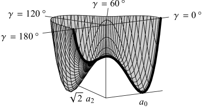
Figure 1: The GCM potential function for $d$$<$0 posesses a global minimum, a saddle point, and a local maximum at $\beta$=0. The case $d$=$-5$ is shown here as an example, plotted as a function of the Cartesian coordinates $(a_{0},\sqrt{2}a_{2})$ or polar coordinates $(\beta,\gamma)$, for $\gamma$=0^∘ to 180^∘. The cut along the $a_{0}$-axis (thick line) is the same as is shown in the second panel of Fig. 2. The global minimum is visible in this figure at $\gamma$=0^∘ and 120^∘, and the saddle point is visible at $\gamma$=60^∘ and 180^∘. The saddle point is a local minimum with respect to $\beta$ and a local maximum with respect to $\gamma$.

Figure 2: Illustration of the qualitatively different shapes of the GCM potential function (6) obtained for different ranges of values for the parameter $d$. Potentials are shown as a function of $\beta$ along the $a_{0}$-axis cut (see text). For $f$ in MeV, the energy scale is also in MeV.

Figure 3: Scalings of the GCM potential function (6) obtained by changing the values of the parameters $e$ and $f$. The varying parameter $e$ dilates the potential with respect to $\beta$, while varying $f$ applies a multiplicative factor to the potential. Potentials are shown as a function of $\beta$ along the $a_{0}$-axis cut (see text). For $f$ in MeV, the energy scale is also in MeV.

Figure 4: Illustration of the effect of increasing $S$. Increasing $S$ by a factor of 4 relative to the original Hamiltonian (upper left) may be accomplished in various ways: by decreasing the mass parameter $B_{2}$ by a factor of 4 (bottom left), by making the potential narrower by a factor of 2 (top right), or by making the potential shallower by a factor of 4 (bottom right). The effects of each are equivalent (see text).

Extrema along the two rays $\gamma$=0^∘ and $\gamma$=180^∘ are found by identification of the zeroes of $\partial V/\partial\beta$ for $\cos 3\gamma$=+1 and for $\cos 3\gamma$=$-1$. The variable $\beta$ is a radial coordinate and so takes on only positive values. However, the form of the following results is considerably simplified by noting that the only occurrence of $\cos 3\gamma$ in (6) is in a product also containing the only occurrence of an odd power of $\beta$, so substituting $\cos 3\gamma$=$-1$ is algebraically equivalent to setting $\cos 3\gamma$=$+1$ and negating $\beta$. Any extremum occuring for $\cos 3\gamma$=$-1$ will thus be found when the extrema for $\cos 3\gamma$=+1 are sought, but at a fictitious “negative” $\beta$ value. A simple expression for the $\beta$ values yielding extrema along $\gamma$=0^∘ follows, but it must be interpreted with the proviso that when a negative $\beta$ value is encountered it actually represents a positive $\beta$ value along $\gamma$=180^∘. The extrema of $V$ along the $a_{0}$-axis cut are located at

$$\beta=\begin{cases}0,\beta_{-},\beta_{+}&d\leq 1\\ 0&d>1\end{cases}$$ (8)

where

$$\beta_{\pm}=\frac{3}{4}\sqrt{\frac{5}{14}}\left(1\pm r\right)e,$$ (9)

in terms of $r$$\equiv$$\sqrt{1-d}$. The extremal values of the potential are

$$V(\beta_{\pm})=-\frac{135}{50176}(r\pm 1)^{3}(3r\mp 1)f.$$ (10)

The nature of the extrema — whether they are minima, maxima, saddle points, or inflection points — can be ascertained from the signs of the partial derivatives. The extremum structure of the potential depends only upon the value of $d$, as summarized in Fig. 2. For $d$$<$0, the potential has both a global minimum and a saddle point at nonzero $\beta$ (Fig. 1). For 0$<$$d$$<$1, minima are present at both at nonzero $\beta$ and at $\beta$=0, with the deformed minimum lower for 0$<$$d$$<$8/9 and the undeformed minimum lower for 8/9$<$$d$$<$1. For $d$$>$1, there is only one minimum, located at $\beta$=0.

Let us briefly address the ranges of definition for the parameters $e$ and $f$. Negating $e$ reflects the potential about $\beta$=0. A positive value of $e$ places the deformed minimum on the prolate side of the cut ($\beta_{+}$$>$0), while negative $e$ places the deformed minimum on the oblate side of the cut ($\beta_{+}$$<$0). All model predictions for energies and transition strengths are unchanged under interchange of prolate and oblate deformations, and only the signs of quadrupole matrix elements and thus quadrupole moments are affected. Throughout the discussions and examples in the present work, $e$ will be taken positive without loss of generality. Only positive values of $f$ are meaningful, since for $f$ negative the coefficient on the $\beta^{4}$ term in the potential is negative. This makes $V\rightarrow-\infty$ as $\beta\rightarrow\infty$, leaving the system globally unbound. The effects on the potential of varying the parameters $e$ and $f$ are illustrated in Fig. 3.

In terms of the new parameters, overall multiplication of the Hamiltonian by $b$ is obtained by the transformation

$$B_{2}^{\prime}=\frac{1}{b}B_{2}\qquad d^{\prime}=d\qquad e^{\prime}=e\qquad f^{\prime}=bf,$$ (11)

and deepening the potential by $a^{2}$ while dilating by $1/a$ is accomplished by the transformation

$$B_{2}^{\prime}=B_{2}\qquad d^{\prime}=d\qquad e^{\prime}=\frac{1}{a}e\qquad f^{\prime}=a^{2}f.$$ (12)

If two sets of parameter values, call them $(B_{2},d,e,f)$ and $(B_{2}^{\prime},d^{\prime},e^{\prime},f^{\prime})$, can be transformed into each other by any combination of these scaling relations, the solutions for these parameter sets will be identical, to within energy normalization and wave function dilation. If, however, $(B_{2},d,e,f)$ and $(B_{2}^{\prime},d^{\prime},e^{\prime},f^{\prime})$ cannot be transformed into each other by (11) and (12), the solutions for these parameters will be distinct. Parameter sets are thus naturally grouped into “families”, where $(B_{2},d,e,f)$ and $(B_{2}^{\prime},d^{\prime},e^{\prime},f^{\prime})$ are members of the same family if and only if they are related by the scaling transformations (11) and (12).

We are now equipped to construct a “structure parameter” $S$ which is invariant under the transformations (11) and (12). The quantity

$$S\equiv\frac{1}{B_{2}e^{2}f}$$ (13)

may readily be verified to satisfy this condition. If two points in parameter space are characterized by the same values of $d$ and $S$, they yield identical energy spectra, to within an overall normalization factor, and identical wave functions, to within dilation, and consequently identical $B(E2)$ ratios. Two points characterized by different values of $d$ or of $S$ will in general give different energy spectra, wave functions, and $B(E2)$ ratios.

For a given potential shape, given by $d$, the parameter $S$ determines how “high” the levels lie relative to the features of the potential. An increase in $S$ may be achieved by decreasing the mass parameter $B_{2}$, making the potential narrower, or making the potential shallower. Each of these has an equivalent effect on the level spectrum (Fig. 4), causing level energies to rise relative to the potential.

III Mapping the GCM parameter space

The truncated GCM described in Section II is effectively a two-parameter model, with parameters $d$ and $S$. The two other degrees of freedom remaining from the four original parameters provide only an overall normalization factor on the energy scale and, through dilation of the wave functions in the coordinate $\beta$, on the $B(E2)$ strength scale. Because of the simplicity of this model, the behavior of an observable over the entire model space can be summarized on a single contour plot. However, the parameter values needed to cover the structural features of interest span many orders of magnitude, so it is necessary to make some preliminary analytic estimates to guide the numerical calculations if an effective and comprehensive survey of the parameter space is to be made.

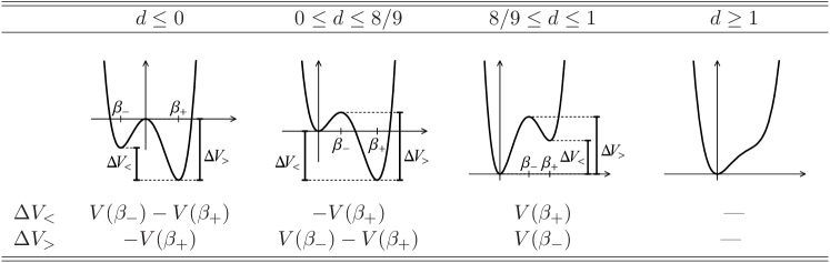
Figure 5: Definitions of the energy differences $\Delta V_{<}$ and $\Delta V_{>}$ between extrema of the GCM potential, for different ranges of $d$ values, in terms of $V(\beta_{\pm})$ [see (10)]. Different structure predictions are obtained for a given potential shape depending upon the energy of the ground state and other low-lying levels relative to the various extrema of the potential. The quantities $\Delta V_{<}$ and $\Delta V_{>}$ are chosen so as to give approximate “boundaries” on the level energies (taken relative to the global minimum of the potential), separating the energies corresponding to different structural regimes described in the text. If low-lying levels have energies substantially less than $\Delta V_{<}$, they are “trapped” in the global minimum. If levels have energies substantially greater than $\Delta V_{>}$, quartic oscillator behavior dominates. Potentials are plotted on the cut along the $a_{0}$-axis.

Figure 6: Estimates $S_{<}(d)$ (dashed line) and $S_{>}(d)$ (solid line) of the $S$ values separating the different structural regimes (see text). The intervals $d\leq 0$ and $0\leq d\leq 1$ are plotted separately for clarity.

Figure 7: Map of the GCM $(d,S)$ parameter space. The regions in which qualitatively different structures occur are indicated. The curves $S=S_{<}$ and $S=S_{>}$ (dotted lines) provide estimates for the approximate boundaries between these regions. Within the rotor-vibrator region, the stiffness for $\beta$ and $\gamma$ vibrations varies with $d$ (double arrow) with a dependence given approximately by (21). Bars along the edges of the plot represent structures which occur in their ideal form at $d\rightarrow\pm\infty$ or at $S\rightarrow 0$ or $\infty$. (“W-J” denotes Wilets-Jean rigidly-deformed $\gamma$-soft structure wilets1956:oscillations .) The $d$- and $S$-axis scales match those of the following figures (Figs. 8 and 9) to facilitate direct comparison with the calculated observable values.

Let us first consider what qualitatively different types of behavior are possible within the model space. Each of the different potential “shapes” depicted in Fig. 2 can give rise to several different types of structure, depending upon the excitation energy of the ground state and other low-lying levels relative to the minimum of the potential. For potentials with $d$$<$0:

1. If level energies lie well below the saddle point, the states are energetically confined to the deformed minimum, yielding rotational behavior.

2. If level energies lie between the saddle point and the local maximum at $\beta$=0, all $\gamma$ values are energetically accessible, but $\beta$=0 is still not accessible. In this case, deformed $\gamma$-soft structure is possible.

3. If level energies lie well above the local maximum at $\beta$=0, the potential controlling the behavior of these states is dominantly a $\beta^{4}$ quartic oscillator well.

For potentials with 0$<$$d$$<$1, two minima are present, one at zero deformation and one at nonzero deformation:

1. If level energies lie well below the higher minimum, the states are energetically confined to the global minimum, yielding rotational behavior for 0$<$$d$$<$8/9 or approximately harmonic oscillator behavior for 8/9$<$$d$$<$1.

2. If level energies lie above both minima but below the saddle point barrier, the energetically-accessible regions around the two minima are separated from each other by this barrier. States involving mixing through the barrier may be possible.

3. If level energies lie well above the barrier, the behavior again approaches that of a quartic oscillator.

Finally, for potentials with $d$$>$1, deformed structure is not possible. If level energies are low in the well, so the states are confined to a region of small $\beta$ where the $\beta^{2}$ term in the potential dominates, harmonic oscillator behavior arises. For level energies much higher in the well, the $\beta^{4}$ term dominates, yielding quartic oscillator behavior.

Thus, for the potentials with $d$$<$1, three different structural regimes are possible at each given value of $d$, and the qualitative nature of the low-lying levels is expected to depend upon the excitation energy of these levels relative to specific extremum features of the potential well. Fig. 5 defines energy differences $\Delta V_{<}$ and $\Delta V_{>}$ describing characteristic energy scales for the structural regimes. If the ground state and other low-lying states occur at energies (measured relative to the lowest point of the potential) substantially below $\Delta V_{<}$, the structure is expected to be that of the lowest-energy regime. For energies near or between $\Delta V_{<}$ and $\Delta V_{>}$, structure in the intermediate regime is possible. And, for energies well above $\Delta V_{>}$, the structure is that of the highest-energy, or quartic oscillator, regime.

Let us estimate the $S$ values, at a given value of $d$, which place the low-lying level energies in each of these ranges. The Wentzel-Kramers-Brillouin approximation (e.g., Ref. messiah1999:qm ) yields a quantization condition

$$\int_{0}^{\beta_{\text{max}}}d\beta\sqrt{B[E-V(\beta)]}\approx\left(n+\frac{3}{4}\right)\hbar\pi,$$ (14)

$n=0,1,2,\ldots$, on the radial coordinate in the five-dimensional Schrödinger equation, ignoring here the five-dimensional equivalent of the centrifugal potential, where the mass $B$ appearing in the usual form of the Schrödinger equation is $\sqrt{5}B_{2}/2$. Since we seek only an order-of-magnitude estimate, let us replace $E-V(\beta)$ in (14) by a constant value $E-\overline{V}$, representing the excitation energy relative to an “average” floor of the well, and consider only the ground state ($n$=0). Then (14) reduces to the condition,

$$\beta_{\text{max}}\approx\frac{1}{2}\frac{2\pi\hbar}{\sqrt{2B(E-\overline{V})}},$$ (15)

or, simply, that approximately one-half of a de Broglie wavelength must fit within the width $\beta_{\text{max}}$ of the well. The appropriate “width” of the GCM potential for this estimate depends upon how “high” the ground state lies within the well. We are now considering the boundaries of the structural regimes, for which the ground state energy lies near the upper extrema in the potential. The location $\beta_{+}$ of the prolate minimum provides a reasonable order-of-magnitude measure of the well width in this case (see Fig. 5). Then (15) indicates that $S$ values of approximately

$$S_{\lessgtr}\approx\frac{1}{\pi^{2}\hbar^{2}}\left(\frac{\Delta V_{\lessgtr}}{f}\right)\left(\frac{\beta_{+}}{e}\right)^{2},$$ (16)

yield ground state energies at the borders $\Delta V_{<}$ and $\Delta V_{>}$ of the structural regimes. The values of $S_{\lessgtr}$ obtained by substituting the expressions for $\Delta V_{\lessgtr}$ from Fig. 5 are functions of $d$ only (Fig. 6).

For $d$$<$8/9, rotational behavior occurs when the levels are at a sufficiently low energy with respect to the potential [$S$$\lesssim$$S_{<}(d)$]. For these rotational nuclei, additional useful analytic estimates can be made of the quantitative dependence of observables on $d$ and $S$. For states sufficiently low-lying (well-confined) in the deformed minimum, the structure approaches that of small oscillations about a deformed equilibrium, which is described analytically in the rotation-vibration model (RVM) faessler1965:rvm . This model provides simple leading-order estimates for the rotational, $\beta$-vibrational, and $\gamma$-vibrational energy scales. The $2^{+}$ state energy for the yrast band is determined by the moment of intertia, giving

$$E_{2g}\approx\frac{\hbar^{2}}{B\beta_{0}^{2}},$$ (17)

where $\beta_{0}$ is the equilibrium deformation. The $\beta$-vibrational and $\gamma$-vibrational excitation energies are determined by the curvature of the potential in each of these degrees of freedom, yielding

$$E_{\beta}\approx\hbar\sqrt{\frac{V_{\beta\beta}}{B}}\qquad E_{\gamma}\approx\hbar\sqrt{\frac{V_{\gamma\gamma}}{B\beta_{0}^{2}}},$$ (18)

where $V_{\beta\beta}$$\equiv$$\partial^{2}V/\partial\beta^{2}$ and $V_{\gamma\gamma}$$\equiv$$\partial^{2}V/\partial\gamma^{2}$. The bandhead state energies are related to $E_{\beta}$ and $E_{\gamma}$ by $E(0^{+}_{\beta})\approx E_{\beta}$ and $E(2^{+}_{\gamma})\approx E_{\gamma}+\frac{1}{3}E_{2g}$ faessler1965:rvm .

These estimates may be evaluated for the GCM potential (6) in a straightforward fashion caprio2003:diss . The vibrational energies normalized to the yrast $2^{+}$ energy are

$$\frac{E_{\beta}}{E_{2g}} \approx\frac{135}{448\sqrt{7}}\sqrt{\frac{r(1+r)^{5}}{\hbar^{2}S}}$$ (19)

$$\frac{E_{\gamma}}{E_{2g}} \approx\frac{135\sqrt{3}}{448\sqrt{7}}\sqrt{\frac{(1+r)^{5}}{\hbar^{2}S}},$$ (20)

in terms of $r$$\equiv$$\sqrt{1-d}$, and the ratio of the $\beta$ and $\gamma$ vibration excitation energies is simply

$$\frac{E_{\beta}}{E_{\gamma}}\approx\sqrt{\frac{r}{3}}.$$ (21)

The ratios (19)–(21) depend only upon $d$ and $S$, as expected from the scaling properties of Section II. These estimates provide guidance, needed for the numerical calculations of the following section, as to both the range of $d$ values of physical interest and the appropriate axis scale or calculational mesh spacing for the parameter $d$. Observe that, by (21), it is expected that “$\beta$-stiff” rotors, with $E_{\beta}$$>$$E_{\gamma}$, occur for $d$$<$$-8$, while “$\gamma$-stiff” rotors, with $E_{\gamma}$$>$$E_{\beta}$, occur for $d$$>$$-8$.

The combined results of this section give a detailed picture of the qualitative characteristics expected for predictions of the truncated GCM and provide quantitative estimates as to where in the $(d,S)$ parameter space these properties are to be found. The results are summarized graphically as a “map” of the parameter space in Fig. 7.

IV Numerical results

Contour plots of several observables over the $(d,S)$ parameter space are shown in Figs. 8 and 9. All observables plotted are ratios of energies or of $B(E2)$ values. As discussed in the previous sections, at a given $(d,S)$ any desired overall normalization for the energy and $B(E2)$ scales can then be obtained by proper rescaling of the well width, well depth, and mass parameter.

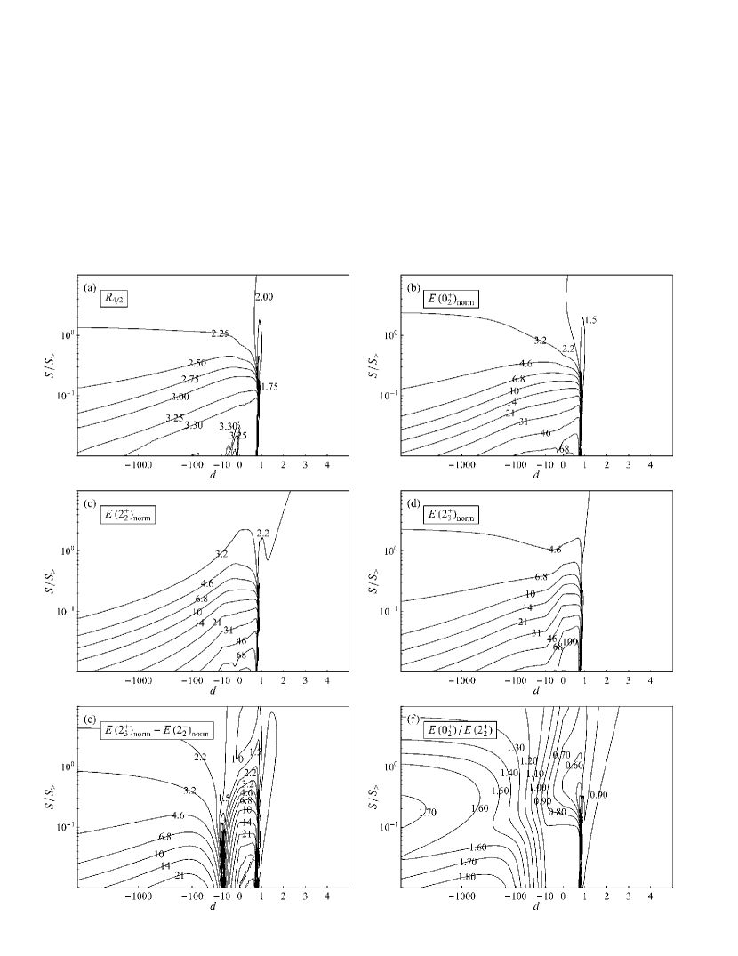
Figure 8: Energy observable predictions of the GCM for $-5000\leq d\leq 5$ and $10^{-2}\leq S/S_{>}\leq 10^{+1}$: (a) $R_{4/2}$$\equiv$$E(4^{+}_{1})/E(2^{+}_{1})$, (b) $E(0^{+}_{2})_{\mathrm{norm}}$$\equiv$$E(0^{+}_{2})/E(2^{+}_{1})$, (c) $E(2^{+}_{2})_{\mathrm{norm}}$$\equiv$$E(2^{+}_{2})/E(2^{+}_{1})$, and (d) $E(2^{+}_{3})_{\mathrm{norm}}$$\equiv$$E(2^{+}_{3})/E(2^{+}_{1})$. For examination of the crossing of the $\beta$ and $\gamma$ bands (see text), it is also useful to plot the quantities (e) $[E(2^{+}_{3})-E(2^{+}_{2})]/E(2^{+}_{1})$ and (f) $E(0^{+}_{2})/E(2^{+}_{2})$.

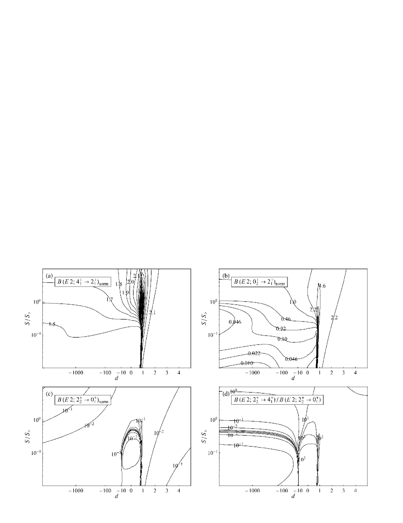
Figure 9: $B(E2)$ observable predictions of the GCM for $-5000\leq d\leq 5$ and $10^{-2}\leq S/S_{>}\leq 10^{+1}$: (a) $B(E2;4^{+}_{1}\rightarrow 2^{+}_{1})_{\mathrm{norm}}$$\equiv$$B(E2;4^{+}_{1}\rightarrow 2^{+}_{1})/B(E2;2^{+}_{1}\rightarrow 0^{+}_{1})$, (b) $B(E2;0^{+}_{2}\rightarrow 2^{+}_{1})_{\mathrm{norm}}$$\equiv$$B(E2;0^{+}_{2}\rightarrow 2^{+}_{1})/B(E2;2^{+}_{1}\rightarrow 0^{+}_{1})$, (c) $B(E2;2^{+}_{2}\rightarrow 0^{+}_{1})_{\mathrm{norm}}$$\equiv$$B(E2;2^{+}_{2}\rightarrow 0^{+}_{1})/B(E2;2^{+}_{1}\rightarrow 0^{+}_{1})$, and (d) $B(E2;2^{+}_{2}\rightarrow 4^{+}_{1})/B(E2;2^{+}_{2}\rightarrow 0^{+}_{1})$. $B(E2)$ values are calculated using the linear form of the electric quadrupole operator.

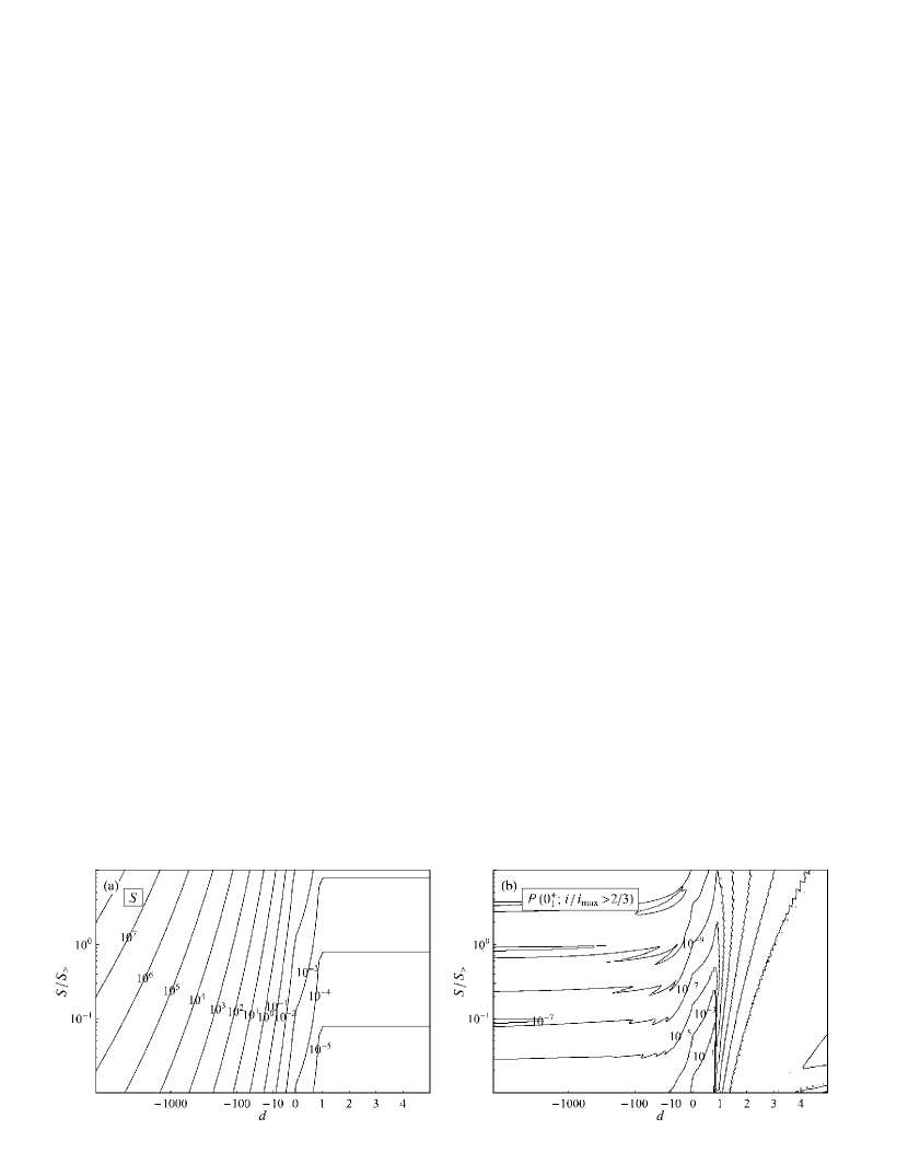
Figure 10: Auxiliary plots for $-5000\leq d\leq 5$ and $10^{-2}\leq S/S_{>}\leq 10^{+1}$: (a) $S$ values (in $10^{42}\,\mathrm{MeV}^{-2}\mathrm{s}^{-2}$) for the calculations of Figs. 8 and 9, to allow $S$ parameter values to be read directly, rather than as $S/S_{>}$, for points on these plots, and (b) the total probability content of the highest (by phonon number) 1/3 of basis states for the calculated $0^{+}_{1}$ state, as an indicator of convergence (see text).

The $d$-axis in Figs. 8 and 9 extends from $d$=$-5000$ to 5. Inclusion of the low end of this range is necessary to allow description of rotational nuclei with high-lying $\beta$ vibrations (21). In order to encompass this full range while maintaining a reasonably detailed view of the region around $d$=0 in the plots, it is helpful to use a nonlinear $d$-axis scale for $d<0$. The estimate of $E_{\beta}/E_{\gamma}$ in (21) indicates that this observable varies as $(1-d)^{1/4}$, so for $d<0$ the $d$-axis of Figs. 8 and 9 is chosen to be linear in $(1-d)^{1/4}$.

In the range of $d$ values being considered, the $S$ values resulting in pheonomena of interest span approximately fourteen orders of magnitude, as seen from Fig. 6. This occurs since $S$ is defined in terms of $e$ and $f$, and the values of these parameters needed to construct a reasonably-sized potential vary greatly with $d$ (see Fig. 2 for examples). However, at any particular value of $d$, only about three decades in $S$, those immediately surrounding $S$=$S_{>}(d)$, contain predictions of interest. To make effective use of plotting space, the $S$-axis in Figs. 8 and 9 is expanded to show only $10^{-2}S_{>}(d)\leq S\leq 10^{+1}S_{>}(d)$ at each point along the $d$-axis. Fig. 10(a) facilitates the reading of $S$ directly off the contour plots.

Energy observables are shown in Fig. 8. The values of the ratio $R_{4/2}\equiv E(4^{+}_{1})/E(2^{+}_{1})$ [Fig. 8(a)], an observable which serves as a basic indicator of structure, closely match the values expected from the $S_{<}$ and $S_{>}$ estimates. The region with 2.2$<$$R_{4/2}$$<$2.6 corresponds approximately to that between the dotted lines representing $S_{<}$ and $S_{>}$ in Fig. 7, in which deformed $\gamma$-soft structure is expected. For the rotational-vibrational nuclei, found in the lower left-hand region of the plots, the observables $E(0^{+}_{2})/E(2^{+}_{1})$, $E(2^{+}_{2})/E(2^{+}_{1})$, and $E(2^{+}_{3})/E(2^{+}_{1})$ [Fig. 8(b-d)] reflect the basic dependences of the $\beta$ and $\gamma$ excitation energies estimated in (19) and (21). At a given $d$, the excited band energies increase relative to $E(2^{+}_{1})$ as $S$ decreases. Degeneracy of the $\beta$ and $\gamma$ excitations is expected at $d$$\approx$$-8$, and this behavior is clearly visible from the sharp minimum in $[E(2^{+}_{3})-E(2^{+}_{2})]/E(2^{+}_{1})$ [Fig. 8(e)], where an avoided level crossing occurs. To the left of this division, the $2^{+}_{2}$ state is the $\gamma$-vibrational bandhead; whereas, to the right of this division, the $2^{+}_{2}$ state is the $\beta$-vibrational $2^{+}$ band member. Proceeding to the left of the band crossing, the $0^{+}_{2}$ level energy rises relative to the $2^{+}_{2}$ energy [Fig. 8(f)], as expected, due to increasing $\beta$ stiffness. The $0^{+}_{2}$ energy saturates at $\lesssim 2E(2^{+}_{2})$, however, since as the $\beta$ vibrational excitation continues to rise it leaves the two-phonon $\gamma$-vibrational state as the lowest $K=0$ excitation (see Ref. faessler1965:rvm ).

$B(E2)$ observable predictions are shown in Fig. 9. The ratio $B(E2;4^{+}_{1}\rightarrow 2^{+}_{1})/B(E2;2^{+}_{1}\rightarrow 0^{+}_{1})$ [Fig. 9(a)] varies essentially smoothly from rotational values to harmonic oscillator values, except that extreme large and small values are encountered in a narrow region between $d\approx 0.8$ and $d\approx 0.9$. In this region, structures involving coexistence in multiple minima are expected, so the $2^{+}_{1}$ and $4^{+}_{1}$ levels do not necessarily correspond to the same structure. Numerical convergence may also not be occurring for certain calculations in this region, as discussed below. The observable $B(E2;0^{+}_{2}\rightarrow 2^{+}_{1})/B(E2;2^{+}_{1}\rightarrow 0^{+}_{1})$ [Fig. 9(b)] is of interest as the $\beta$-vibrational decay strength for rotational nuclei. In the region $d$$\lesssim$$-8$, $B(E2;2^{+}_{2}\rightarrow 0^{+}_{1})/B(E2;2^{+}_{1}\rightarrow 0^{+}_{1})$ [Fig. 9(c)] is the $\gamma$-vibrational decay strength. The predictions for the observable $B(E2;2^{+}_{2}\rightarrow 4^{+}_{1})/B(E2;2^{+}_{2}\rightarrow 0^{+}_{1})$ [Fig. 9(d)] may be compared with the “Alaga ratio” predictions for true rotors bohr1998:v2 , those for the $2^{+}_{\gamma}$ state if $d$$\lesssim$$-8$ or for the $2^{+}_{\beta}$ state if $d$$\gtrsim$$-8$.

Numerical diagonalization of the GCM Hamiltonian is susceptible to convergence failure gneuss1971:gcm ; margetan1982:basis-optimization . The code of Ref. troltenier1991:gcm , used for the present calculations, obtains eigenvalues and eigenfunctions by diagonalization in a basis of five-dimensional harmonic oscillator wave functions. If the set of basis functions chosen is not sufficiently complete or is not adequately matched in radial extent to the eigenfunctions it is being used to approximate, the process fails to correctly calculate the GCM predictions for the eigenvalues and eigenfunctions. The basis is characterized by the phonon number $N$ at which it is truncated and by the stiffness parameter $s\equiv(B_{2}C_{2}/\hbar^{2})^{1/4}$ of the oscillator from which it is constructed, which controls the radial extent of the basis functions. For the present calculations, the basis was truncated at $N$=30, and $s$ was automatically optimized by the variational procedures of Refs. margetan1982:basis-optimization ; troltenier1991:gcm .

Significant probability in the highest basis functions indicates that the solution has “overflowed” the truncated basis and that the results of the diagonalization are not reliable. For successfully convergent diagonalizations, most of the probability density is concentrated in the “lowest” (by oscillator phonon number) $\sim$10$\%$ of the basis functions gneuss1971:gcm ; margetan1982:basis-optimization . Fig. 10(b) provides a contour plot of the probability content of the “highest” 1/3 of basis states for the calculated $0^{+}_{1}$ state. Large values ($\gtrsim$$10^{-3}$) indicate a calculation for which nonconvergence is likely to have occured. However, this quantity is only a partial indicator of convergence, and it does not provide a substitute for detailed convergence studies gneuss1971:gcm ; margetan1982:basis-optimization to determine the actual extent of convergence for each excited state.

Convergence failure occurs for some of the most sharply deformed structures covered by Figs. 8 and 9. At very low $S$ values in the rotor region, where the most clearly well-deformed structure occurs and $R_{4/2}$ should approach 3.33, the numerical calculations instead exhibit sporadic patches of sharp fall-off in the $R_{4/2}$ value [Fig. 8(a), at $d\lesssim 0$]. Comparison with Fig. 10(b) shows that these calculations exhibit relatively high probability contents for the highest 1/3 of basis functions. Convergence failure also occurs for parameter sets near $d=0.8$, where coexistence in multiple minima occurs.

Application of the results described in this article requires the use of meshes of calculations to produce contour plots of observable values, such as those of Figs. 8 and 9. To facilitate this process, a database has been made available through the Electronic Physics Auxiliary Publication Service (EPAPS) epaps , containing energy and $B(E2)$ observables for low-lying states from a mesh of calculations covering the ($d$,$S$) parameter space considered here. An accompanying computer program is provided to extract observable values from this database, calculate arbitrary expressions involving these observables, and tabulate them in formats commonly accepted by contour plotting codes. The mesh consists of 150 steps along the $d$-axis and 100 along the $S$-axis, uniformly distributed with respect to the axis scalings described above. Further details may be found in the EPAPS documentation epaps .

V Illustration of the approach: $\mathbf{{}^{102}\mathrm{Pd}}$

The geometric collective model is most useful for the interpretation of transitional nuclei, to which the simple models for limiting structures (e.g., the harmonic oscillator or rotor models) cannot readily be applied. The Pd isotopes provide an example of a spherical to deformed $\gamma$-soft structural transition and have been extensively modeled as transitional nuclei using the interacting boson model (IBM) stachel1982:ibm ; bucurescu1986:ibm ; pan1998:so6u5 , the IBM-2 vanisacker1980:ibm ; kim1996:ibm ; giannatiempo1998:ibm , and other collective models vorov1985:quartic .

Figure 11: Experimental level scheme and $B(E2)$ strengths for ¹⁰²Pd, alongside the E(5) predictions and the GCM predictions for $d$=$-43$ and $S$=56$\times 10^{42}\,\mathrm{MeV}^{-2}\mathrm{s}^{-2}$, normalized to the experimental $E(2^{+}_{1})$ and $B(E2;2^{+}_{1}\rightarrow 0^{+}_{1})$ values. Observed levels with no clear theoretical counterpart or calculated levels with no clear experimental counterpart (see text) are indicated with dashed lines. Experimental $B(E2)$ strengths are from Refs. zamfir2002:102pd-beta ; nds1998:102 ; luontama1986:102pd104pd-p2n-ppprime-coulex , with the assumption of pure $E2$ multipolarity if the multipolarity is not otherwise known. $B(E2)$ values in brackets are relative values, while all others are absolute values in W.u.

Recent spectroscopic measurements on ¹⁰²Pd zamfir2002:102pd-beta have clarified the scheme of low-lying levels and provided a detailed set of information on $B(E2)$ strengths among these levels. The data of Ref. zamfir2002:102pd-beta support the description of ¹⁰²Pd as $\gamma$-soft and softly-deformed with respect to $\beta$. The low-lying levels approximate an O(5) multiplet structure (Fig. 11), as expected for a $\gamma$-independent potential rakavy1957:gsoft . A reasonable description zamfir2002:102pd-beta is obtained with the E(5) model of Iachello iachello2000:e5 , in which the Bohr Hamiltonian is used with a potential which is $\gamma$-soft and flat (a square well) with respect to $\beta$. There are, however, discrepancies, which may be addressed using the present formulation of the GCM.

Let us first summarize the description of ¹⁰²Pd obtained in Ref. zamfir2002:102pd-beta . Levels occur at approximately the correct energies to constitute the $4^{+}$-$2^{+}$ members of a $\tau$=2 multiplet and the $6^{+}$-$4^{+}$-$3^{+}$ members of a $\tau$=3 multiplet in a $\gamma$-soft description (Fig. 11). The $R_{4/2}$ energy ratio value of 2.29 suggest a structure intermediate between that of the harmonic oscillator ($R_{4/2}$=2.0) and a Wilets-Jean rigidly-deformed $\gamma$-soft structure ($R_{4/2}$=2.5) wilets1956:oscillations . The data of Ref. zamfir2002:102pd-beta indicate that the “allowed” $\Delta\tau$=$-1$ transitions from the $4^{+}_{\tau=3}$ and $3^{+}_{\tau=3}$ levels are greatly enhanced over the “forbidden” $\Delta\tau$=$-2$ transitions, although some necessary $M1$/$E2$ mixing ratios have not been measured.

The low-lying, isomeric $0^{+}_{2}$ level at 1593 keV is identified as a likely intruder state. An inspection of the evolution of level energies along the $N$=56 isotonic chain reveals that the $0^{+}_{2}$ energy decreases towards the $Z$=40 shell closure (Fig. 12), indicating that this is not an ordinary collective state constructed from the $Z$=40–50 valence space. The evolution is consistent with that of a collective excitation involving the entire $Z$=28–50 shell, breaking the subshell closure at $Z$=40. The next excited $0^{+}$ level, at 1658 keV, lies at an energy 2.98 times the $2^{+}_{1}$ level energy, in near perfect agreement with the E(5) prediction [$E(0^{+}_{2})$=3.03$E(2^{+}_{1})$]. This level decays with collective $E2$ strength to the $2^{+}_{1}$ level [13(3) W.u.], as expected for the head of the $\xi$=2 family, though this strength is lower than predicted [28(2) W.u.] by the E(5) model. A $0^{+}$ member of the $\tau$=3 multiplet must be found for this picture to be complete.

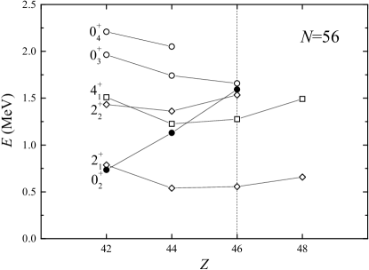
Figure 12: Evolution of level energies for low-lying states along the $N$=56 isotonic chain. The contrary behavior of the $0^{+}_{2}$ state (filled symbols), with a decreasing energy towards the $Z$=40 shell closure, indicates a cross-shell intruder nature. The dotted line indicates $Z$=46 (Pd). (Figure based upon Ref. zamfir2002:102pd-beta .)

However, several differences in quantitative detail are present between experiment and the pure $\gamma$-soft predictions, as can be seen from Fig. 11. Some of the main deviations from this picture are:

1. The $4^{+}$ and $2^{+}$ members of the proposed $\tau$=2 multiplet are split in energy, with the $4^{+}$ level lower.

2. The absolute $B(E2;2^{+}_{\tau=2}\rightarrow 2^{+}_{\tau=1})$ strength is lower than the $B(E2;4^{+}_{\tau=2}\rightarrow 2^{+}_{\tau=1})$ strength.

3. Both the $3^{+}_{\tau=3}$ and $4^{+}_{\tau=3}$ states show a strong preference to decay to the $2^{+}_{\tau=2}$ state rather than to the $4^{+}_{\tau=2}$ state. Only a slight such preference is expected for $\gamma$-soft structure.

These deviations from the E(5) model predictions are qualitatively consistent with the incipient formation of a $\gamma$ band. Such structure would arise if the potential were perturbed from E(5) to impose a slight preference for axial symmetry.

To consider this perturbation quantitatively, let us make use of the truncated GCM. The choice of values for the parameters $d$ and $S$ is constrained simply by the requirement that the low-lying energy observables be reproduced. It is desirable to retain the good agreement with the experimental $4^{+}_{\tau=2}$ level energy, $\tau$=3 multiplet energy, and first excited $0^{+}$ level energy obtained with the E(5) description while also reproducing the splitting of the $\tau$=2 multiplet. Contours indicating the regions in GCM ($d$,$S$) parameter space for which the predictions match the experimental $R_{4/2}$, $E(2^{+}_{2})/E(2^{+}_{1})$, $E(4^{+}_{2})/E(2^{+}_{1})$, and $E(0^{+}_{2})/E(2^{+}_{1})$ values are shown in Fig. 13. We seek a point in parameter space simultaneously satisfying these conditions. Values for other energy and $B(E2)$ observables could be used to refine the choice, but we are interested here primarily in the general nature of the GCM predictions. The parameter values $d$$\approx$$-43$ and $S$$\approx$56$\times 10^{42}\,\mathrm{MeV}^{-2}\mathrm{s}^{-2}$ constitute a reasonable compromise.

Figure 13: Regions in the ($d$,$S$) parameter space for which the GCM predictions of selected observables match the values found in ¹⁰²Pd: $R_{4/2}$=2.29 to within 2$\%$ (solid line), $E(2^{+}_{2})/E(2^{+}_{1})$=2.75 to within 5$\%$ (dashed line), $E(4^{+}_{2})/E(2^{+}_{1})$=3.84 to within 5$\%$ (dashed-dotted line), and $E(0^{+}_{2})/E(2^{+}_{1})$=2.98 to within 5$\%$ (dotted line). The solid circle indicates $d$=$-43$ and $S$=56$\times 10^{42}\,\mathrm{MeV}^{-2}\mathrm{s}^{-2}$, the parameter values discussed in the text.

The GCM predictions for these values of $d$ and $S$ are shown in Fig. 11 (right). The $4^{+}_{1}$-$2^{+}_{2}$ splitting and low-lying level energies are well reproduced, although some splitting is introduced between the $6^{+}_{1}$, $4^{+}_{2}$, and $3^{+}_{1}$ “multiplet” levels. The $B(E2)$ strengths for the $2^{+}_{2}\rightarrow 2^{+}_{1}$, $4^{+}_{2}\rightarrow 4^{+}_{1}$, and $3^{+}_{1}\rightarrow 4^{+}_{1}$ transitions are all reduced relative to the E(5) predictions, while the other transition strengths in Fig. 11 are relatively unaffected. The change in the predicted strengths for these three transitions is in the correct sense to bring them closer to the experimental values but leaves these strengths still a factor of two to three greater than observed. As noted above, one of the other outstanding issues regarding the interpretation of ¹⁰²Pd in the context of the E(5) picture is the nonobservation of any $0^{+}$ member of the proposed $\tau$=3 multiplet. In the GCM calculation, the $0^{+}_{3}$ level is predicted to be substantially higher in energy than the $6^{+}_{1}$, $4^{+}_{2}$, and $3^{+}_{1}$ states. The potential for the GCM calculation for ¹⁰²Pd is plotted in Fig. 14, showing the extent of the gentle minimum with respect to $\gamma$ at $\gamma$=0^∘.

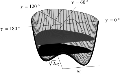
Figure 14: Plot of the potential energy surface for the GCM calculation for ¹⁰²Pd ($d$=$-43$, $S$=56$\times 10^{42}\,\mathrm{MeV}^{-2}\mathrm{s}^{-2}$) as a function of the shape coordinates, showing the $0^{+}_{1}$ and $0^{+}_{2}$ level energies (lower and upper laminae).

VI Conclusion

The general approach and specific techniques discussed in this article recast the GCM, with truncated Hamiltonian, as a very tractable model for theoretical studies and practical application. The use of analytic scaling relations reduces the effective dimensionality of the parameter space for this model, and basic estimates of the parameter dependence of structural properties further simplify navigation of this parameter space. The parameter values most appropriate for the description of a given nucleus can be deduced by inspection of contour plots such as those in Figs. 8 and 9. To facilitate application of these results, a database of calculations covering the model space and a computer code for extracting observable values are provided through the EPAPS epaps .

*

Appendix A

An elementary proof is provided of the scaling property used in Section II, that, for the Schrödinger equation in $n$ dimensions, “deepening” and “narrowing” a potential in the correct proportion simply multiplies all eigenvalues by an overall factor and dilates all eigenfunctions.

Consider the Schrödinger equation in the $n$ Cartesian coordinates $x_{1},\ldots,x_{n}$, with a kinetic energy operator having the standard Cartesian form and a potential energy operator which depends only upon the coordinates,

$$\left[\sum_{i=1}^{n}\left(-\frac{\hbar^{2}}{2m_{i}}\frac{\partial^{2}}{\partial x_{i}^{2}}\right)+V(x_{1},\ldots,x_{n})-E\right]\\ \times\Psi(x_{1},\ldots,x_{n})=0,$$ (22)

where the $m_{i}$ are constants, $V$ is the potential energy operator, and $E$ is the energy eigenvalue for wave function $\Psi$. Suppose that this equation is satisfied by a particular function $\Psi$, with eigenvalue $E$, for a specific potential $V$. Now consider the related expression obtained by substituting the quantities

$$V^{\prime}(x_{1},\ldots,x_{n}) =a^{2}V(ax_{1},\ldots,ax_{n})$$ (23)

$$\Psi^{\prime}(x_{1},\ldots,x_{n}) =\sqrt{a^{n}}\Psi(ax_{1},\ldots,ax_{n})$$

$$E^{\prime} =a^{2}E$$

for the corresponding quantities in (22). This yields

$$\Bigg{[}\sum_{i=1}^{n}\Bigg{(}-\frac{\hbar^{2}}{2m_{i}}\frac{\partial^{2}}{\partial x_{i}^{2}}\Bigg{)}+a^{2}V(ax_{1},\ldots,ax_{n})-a^{2}E\Bigg{]}\\ \times\sqrt{a^{n}}\Psi(ax_{1},\ldots,ax_{n}).$$ (24)

With the substitution $u_{i}=ax_{i}$, this becomes

$$\Bigg{[}\sum_{i=1}^{n}\Bigg{(}-\frac{\hbar^{2}}{2m_{i}}a^{2}\frac{\partial^{2}}{\partial u_{i}^{2}}\Bigg{)}+a^{2}V(u_{1},\ldots,u_{n})-a^{2}E\Bigg{]}\\ \times\sqrt{a^{n}}\Psi(u_{1},\ldots,u_{n}),$$ (25)

which vanishes identically for all values of $(u_{1},\ldots,u_{n})$, by (22). Thus, the dilated wave function $\Psi^{\prime}$ satisfies the Schrödinger equation with the same kinetic energy operator as in (22) but with the modified potential $V^{\prime}$, and does so with eigenvalue $E^{\prime}$. The factor $\sqrt{a^{n}}$ included in the definition of $\Psi^{\prime}$ serves to preserve normalization with respect to the volume element $dx_{1}\cdots dx_{n}$.

It is often convenient to use $n$-dimensional spherical coordinates $(r,\Omega)$, where $r=(x_{1}^{2}+\cdots+x_{n}^{2})^{1/2}$ and $\Omega$ represents the angular coordinates. (These correspond to polar or spherical coordinates in the specific cases $n$=2 or $n$=3, respectively.) In these coordinates, the transformation is $V^{\prime}(r,\Omega)=a^{2}V(ar,\Omega)$ and $\Psi^{\prime}(r,\Omega)=\sqrt{a^{n}}\Psi(ar,\Omega)$, which preserves normalization with respect to the volume element $r^{n-1}drd\Omega$.

The matrix elements of the operator $r^{q}$ are encountered in the determination of electromagnetic transition strengths, so it is useful to derive their properties under dilation. Consider the radial integral

$$I^{AB}=\int_{0}^{\infty}r^{n-1}dr\,[\Psi^{A}(r)]^{*}\,r^{q}\,[\Psi^{B}(r)],$$ (26)

where the angular variables have been suppressed for simplicity. Then the radial integral for the corresponding transformed eigenfunctions,

$${I^{AB}}^{\prime}=\int_{0}^{\infty}r^{n-1}dr\,[\sqrt{a^{n}}\Psi^{A}(ar)]^{*}\,r^{q}\,[\sqrt{a^{n}}\Psi^{B}(ar)],$$ (27)

is related to the original integral by

$${I^{AB}}^{\prime}=a^{-q}I^{AB},$$ (28)

as can be shown by means of a simple change of variable $u=ar$. This property applies to any operator homogeneous of order $q$ in the coordinates, such as each term contributing to the quadrupole operator (3).

The leading-order kinetic energy term in the GCM Hamiltonian (1), substituting the canonical momenta $\pi_{2\mu}$$=$$-i\hbar\partial/\partial\alpha_{2\mu}$, is $-\hbar^{2}/(\sqrt{5}B_{2})\sum_{\mu}\partial^{2}/(\partial\alpha_{2\mu}\partial\alpha^{*}_{2\mu})$. This is not manifestly Cartesian, due to the presence of mixed partial derivatives, but a simple change of variables rakavy1957:gsoft ; eisenberg1987:v1 recasts it in Cartesian form, so the above results may be used. The “radial” coordinate to which the scaling property applies is $\beta$.

References

- (1) G. Gneuss, U. Mosel, and W. Greiner, Phys. Lett. B 30, 397 (1969).
- (2) G. Gneuss, U. Mosel, and W. Greiner, Phys. Lett. B 31, 269 (1970).
- (3) G. Gneuss and W. Greiner, Nucl. Phys. A 171, 449 (1971).
- (4) J. M. Eisenberg and W. Greiner, Nuclear Models: Collective and Single-Particle Phenomena, Vol. 1 of Nuclear Theory (North-Holland, Amsterdam, 1987), 3rd ed.
- (5) A. Bohr and B. R. Mottelson, Nuclear Deformations, Vol. 2 of Nuclear Structure (World Scientific, Singapore, 1998).
- (6) P. O. Hess, M. Seiwert, J. Maruhn, and W. Greiner, Z. Phys. A 296, 147 (1980).
- (7) D. Troltenier, P. O. Hess, and J. A. Maruhn, in Computational Nuclear Physics 1: Nuclear Structure, edited by K. Langanke, J. A. Maruhn, and S. E. Koonin (Springer-Verlag, Berlin, 1991), p. 105.
- (8) P. O. Hess, J. Maruhn, and W. Greiner, J. Phys. G 7, 737 (1981).
- (9) U. Mosel and W. Greiner, Z. Phys. 217, 256 (1968).
- (10) K. Kumar, Nucl. Phys. A 231, 189 (1974).
- (11) J. M. Eisenberg and W. Greiner, Microscopic Theory of the Nucleus, Vol. 3 of Nuclear Theory (North-Holland, Amsterdam, 1976), 2nd ed.
- (12) L. von Bernus, A. Kappatsch, V. Rezwani, W. Scheid, U. Schneider, M. Sedlmayr, and R. Sedlmayr, in Heavy-Ion, High-Spin States and Nuclear Structure (IAEA, Vienna, 1975), Vol. 2, p. 3.
- (13) Jing-ye Zhang, R. F. Casten, and N. V. Zamfir, Phys. Lett. B 407, 201 (1997).
- (14) D. Troltenier, J. P. Draayer, B. R. S. Babu, J. H. Hamilton, A. V. Ramayya, and V. E. Oberacker, Nucl. Phys. A 601, 56 (1996).
- (15) See EPAPS Document No. E-PRVCAN-68-031311 for a database of calculations covering the (,) model space and an accompanying computer program for extracting observable values. This document may be retrieved via the EPAPS home page (http://www.aip.org/pubservs/epaps.html) or by FTP (ftp://ftp.aip.org/epaps/).
- (16) P. Petkov, A. Dewald, and W. Andrejtscheff, Phys. Rev. C 51, 2511 (1995).
- (17) L. von Bernus, diploma thesis, Univ. Frankfurt am Main (1971), as quoted in Ref. habs1974:gcm-n50to82 .
- (18) D. Habs, H. Klewe-Nebenius, K. Wisshak, R. Löhken, G. Nowicki, and H. Rebel, Z. Phys. 267, 149 (1974).
- (19) W. Greiner, Z. Phys. 172, 386 (1963).
- (20) H. L. Acker, dissertation, Phys. Inst. Univ. Freiburg/Breisgau (1965), as quoted in Ref. eisenberg1987:v1 .
- (21) L. Wilets and M. Jean, Phys. Rev. 102, 788 (1956).
- (22) A. Messiah, Quantum Mechanics (Dover, Mineola, New York, 1999).
- (23) A. Faessler, W. Greiner, and R. K. Sheline, Nucl. Phys. 70, 33 (1965).
- (24) M. A. Caprio, dissertation, Yale University (2003).
- (25) F. J. Margetan and S. A. Williams, Phys. Rev. C 25, 1602 (1982).
- (26) J. Stachel, P. Van Isacker, and K. Heyde, Phys. Rev. C 25, 650 (1982).
- (27) D. Bucurescu, G. Căta, D. Cutoiu, G. Constantinescu, M. Ivaşcu, and N. V. Zamfir, Z. Phys. A 324, 387 (1986); 327, 241(E) (1987).
- (28) Feng Pan and J. P. Draayer, Nucl. Phys. A 636, 156 (1998).
- (29) P. Van Isacker and G. Puddu, Nucl. Phys. A 348, 125 (1980).
- (30) K. Kim, A. Gelberg, T. Mizusaki, T. Otsuka, and P. von Brentano, Nucl. Phys. A 604, 163 (1996).
- (31) A. Giannatiempo, A. Nannini, and P. Sona, Phys. Rev. C 58, 3316 (1998).
- (32) O. K. Vorov and V. G. Zelevinsky, Nucl. Phys. A 439, 207 (1985).
- (33) N. V. Zamfir, M. A. Caprio, R. F. Casten, C. J. Barton, C. W. Beausang, Z. Berant, D. S. Brenner, W. T. Chou, J. R. Cooper, A. A. Hecht, R. Krücken, H. Newman, J. R. Novak, N. Pietralla, A. Wolf, and K. E. Zyromski, Phys. Rev. C 65, 044325 (2002).
- (34) D. de Frenne and E. Jacobs, Nucl. Data Sheets 83, 535 (1998).
- (35) M. Luontama, R. Julin, J. Kantele, A. Passoja, W. Trzaska, A. Bäcklin, N.-G. Jonsson, and L. Westerberg, Z. Phys. A 324, 317 (1986).
- (36) G. Rakavy, Nucl. Phys. 4, 289 (1957).
- (37) F. Iachello, Phys. Rev. Lett. 85, 3580 (2000).