Relativistic $O(q^{4})$ two-pion exchange
nucleon-nucleon potential:
configuration space

Abstract

We have recently performed a relativistic $O(q^{4})$ chiral expansion of the two-pion exchange $NN$ potential, and here we explore its configuration space content. Interactions are determined by three families of diagrams, two of which involve just $g_{A}$ and $f_{\pi}$, whereas the third one depends on empirical coefficients fixed by subthreshold $\pi N$ data. In this sense, the calculation has no adjusted parameters and gives rise to predictions, which are tested against phenomenological potentials. The dynamical structure of the eight leading non-relativistic components of the interaction is investigated and, in most cases, found to be clearly dominated by a well defined class of diagrams. In particular, the central isovector and spin-orbit, spin-spin, and tensor isoscalar terms are almost completely fixed by just $g_{A}$ and $f_{\pi}$. The convergence of the chiral series in powers of the ratio (pion mass/nucleon mass) is studied as a function of the internucleon distance and, for $r>$ 1 fm, found to be adequate for most components of the potential. An important exception is the dominant central isoscalar term, where the convergence is evident only for $r>$ 2.5 fm. Finally, we compare the spatial behavior of the functions that enter the relativistic and heavy baryon formulations of the interaction and find that, in the region of physical interest, they differ by about 5%.

I introduction

The research programme for the study of nuclear interactions was outlined more than fifty years ago, in a seminal paper by Taketani, Nakamura, and Sasaki [1]. Pions, then recently detected, were identified as the relevant degrees of freedom for the construction of a theoretical potential. One pion exchanges would dominate at large distances, the exchanges of two uncorrelated pions would come next, and a square well could be used to simulate short range processes. It is quite remarkable that these ideas could stand for such a long time, survive the QCD revolution, and still remain as the qualitative framework of contemporary research. On the other hand, when the $NN$ research programme was first established, no precise information concerning the intrinsic structure of pions and their interactions with nucleons was available. It took about forty years of intense collective work, both experimental and theoretical, for this aspect of the problem to be tamed, with the formulation of chiral perturbation theory (ChPT).

The present day rationale for describing nuclear interactions by means of chiral symmetry is that low energy processes are strongly dominated by the quarks $u$ and $d$ and one may work with a two-flavor QCD. As the masses of these quarks are small in the GeV scale, one treats them as perturbations in a massless Lagrangian. The theory is symmetric under the Poincaré group and, in this limit, also invariant under both isospin and chiral SU(2)$\times$ SU(2) transformations. This last symmetry is realized in the Nambu-Goldstone mode and the QCD vacuum contains a condensate, that allows collective excitations, identified as pions. The non-Abelian character of QCD prevents low energy perturbative calculations and, in practice, one works with chiral effective theories, in which point-like baryons interact by exchanging pions that have small masses.

The one-pion exchange potential (OPEP) became definitively established in the early 1960s and is assumed to dominate completely $NN$ partial waves with orbital angular momentum $L\geq 5$. Its mathematical form was determined in the 1950s and remains stable ever since. One has also learned that any $\pi N$ interaction Lagrangian, based on either pseudoscalar or pseudovector couplings, chiral symmetric or not, yields the very same OPEP. Chiral symmetry is thus irrelevant for this part of the force, as for all single pion processes.

The very opposite happens with the next layer of the interaction, the two-pion exchange potential (TPEP). This component is closely related to the $\pi N$ scattering amplitude and chiral symmetry becomes extremely important. In the 1960s, no perturbative treatment for strong interactions was available [2] and potentials were constructed which incorporated $\pi N$ information by means of dispersion relations [3]. In the same decade, chiral symmetry was being developed in a different framework and, with the help of current algebra techniques, low energy theorems for many pionic amplitudes were derived. Applications of chiral symmetry to $NN$ interactions [4], three-body forces [5], and exchange currents [6] began to be performed in the 1970s. At the end of this decade, Weinberg [7] outlined a research programme based on the idea of ChPT. In the 1980s this theory was fully developed for the meson sector [8] and began to be used in the study of meson-baryon interactions [9].

The systematic use of ChPT in the study of nuclear forces began in the early 1990s, through the works of Weinberg [10] and Ordóñez and van Kolck [11], followed by other authors [12, 13]. These early attempts to construct a chiral TPEP considered only pion and nucleon degrees of freedom and gave rise to poor descriptions of $NN$ data. Realistic potentials require other degrees of freedom, which were introduced in the form of deltas [14], hidden within $\pi N$ subthreshold coefficients [15, 16], or incorporated into low energy constants (LECs) of effective Lagrangians [17, 18, 19, 20, 21]. In spite of apparent differences, there must be a rather important overlap among these various approaches. This is expected because the numerical values of the LECs are normally obtained from empirical $\pi N$ subthreshold coefficients which, in turn, are largely dominated by delta intermediate states [22]. So, to a large extent, one is just using different languages to express the same physics. Support to this view comes from the fact that potentials based on deltas [14], subthreshold coefficients [23], or LECs [17, 18, 19, 24] could produce satisfactory descriptions of asymptotic $NN$ phase shifts, without free parameters. This suggests that, if one could control carefully the peculiarities of the various approaches, the hope of having a TPEP as unique as the OPEP could be realized. This uniqueness is of major theoretical importance, since it would indicate that the effective theory can indeed represent QCD.

In ChPT one uses a typical scale $q$, set by either pion four-momenta or nucleon three-momenta, such that $q\ll 1$ GeV. The leading term of the chiral TPEP is $O(q^{2})$ and, at present, there are two independent expansions of the potential up to $O(q^{4})$ in the literature. The first one is based on heavy baryon chiral perturbation theory (HBChPT) [17, 20], where one uses non-relativistic Lagrangians from the very beginning and the inverse of the nucleon mass $(m)$ as an expansion parameter. Relativistic corrections, needed at $O(q^{4})$, are added separately [21]. The alternative calculation was produced recently by ourselves [25], is covariant, and results were expressed directly in terms of loop integrals and observable subthreshold $\pi N$ coefficients. In the case of $\pi N$ scattering, heavy baryon [26] and relativistic [27, 28] results do not coincide, due to the presence of some diagrams [29, 30] that cannot be represented by series in powers of $q/m$. The same class of diagrams is present in the TPEP and the relativistic potential also cannot be expanded in the heavy baryon series around the point $t=4{\mu}^{2}$. If this restriction is nevertheless ignored and the $q/m$ expansion is performed in the relativistic potential, one recovers most of the structure produced by the heavy baryon formalism. The main discrepancies take the form of both $O(q^{3})$ and $O(q^{4})$ terms, associated, respectively, with the iteration of the OPEP and the Goldberger-Treiman discrepancy. The latter could be easily incorporated into the heavy baryon formalism, whereas the former may derive from the particular definition adopted for the potential, that has to suit a given dynamical equation. In our calculation we treated the iterated OPEP as in Ref.[31].

QCD is a well defined theory and the same should happen when one works at the effective level. In the case of the TPEP, we consider the partial convergence between heavy baryon and covariant results at $O(q^{4})$ as a rather welcome indication that uniqueness may not be too far ahead. The considerable narrowing of the theoretical discussion in the last decade represents a measure of the progress promoted by the systematic use of chiral symmetry, which has allowed one to understand the internal hierarchies of the $NN$ potential in terms of chiral layers. Nevertheless, the question still remains open as to the extent this mathematical picture is backed by nature.

The chiral picture may be assessed by comparing theoretical and empirical phase shifts. In the case of peripheral waves, this can be done perturbatively, without resorting to free parameters, and the main trends are well reproduced [23, 17, 24]. However, these waves are small, error bars are important, and the test is not very stringent. In order to include inner waves, which are larger, one has to use dynamical equations, but this demands the regularization of the chiral potential by means of form factors, since it diverges at large momenta. The problem with form factors is that their use amounts to extending the dynamical content of the potential to higher orders in $q/m$ by means of free parameters, in a way which is not controlled by chiral symmetry. This blurs the chiral content of the potential and success in reproducing data, welcome as it is, also does not represent a very stringent test.

As an interesting alternative, we may assume that the chiral potential, calculated at a given order, determines completely the interaction from a radius $R$ onwards and then use it as an input in phase shift analyses. This would just amount to extending to the TPEP a procedure which has already been used for a long time in the OPEP. For the latter, this idea has proved to be reliable in the elastic regime and for waves with $L\geq 5$. From the standpoint of the symmetry, this happens because chiral corrections are short ranged and one sees just the leading contribution through this window, irrespectively of the order in $q$ one is working at. In the case of the TPEP, the corresponding problem is much more complex and not fully understood. Works along this line have already been performed by the Nijmegen group [18], who claim that a $O(q^{3})$ potential is effective for distances smaller than 2 fm. However, its conclusions are disputed by Entem and Machleidt [32] and the situation remains unclear.

The present paper is motivated by the feeling that the quantitative aspects of chiral hierarchies need to be clearly understood if the TPEP is ever to become a reliable tool to be used in phase shift analyses. Our study is based on the configuration space version of the $O(q^{4})$ potential produced in Ref.[25] and organized as follows. In Sec. II we discuss the dynamical content of the TPEP, which is given by a set of Feynman diagrams, organized into three families. The explicit expressions and corresponding figures for the various components of the potential are given in Sec. III. As the way chiral symmetry is implemented varies with the family considered, in Sec. IV we discuss how dynamics is mapped into the final form of the potential and show that the importance of the LECs is rather channel dependent. Sec. V deals with the convergence of the chiral series and in Sec. VI we discuss the main differences between the relativistic and heavy baryon approaches to the potential. Finally, conclusions are presented in Sec. VII.

II dynamics

FIG. 1.: Two pion exchange amplitude.

The dynamical content of the relativistic $O(q^{4})$ chiral TPEP is determined by the effective Lagrangian

$${\cal L}_{eff}={\cal L}_{\pi}^{(2)}+{\cal L}_{N}^{(1)}+{\cal L}_{N}^{(2)}+{\cal L}_{N}^{(3)}\;,$$ (1)

where ${\cal L}_{\pi}^{(n)}$ and ${\cal L}_{N}^{(n)}$ describe pion-pion and pion-nucleon interactions at $O(q^{n})$. Other degrees of freedom are implicitly taken into account by means of the LECs $c_{i}$ and $d_{i}$, present in ${\cal L}_{N}^{(2)}$ and ${\cal L}_{N}^{(3)}$. The use of covariant Feynman rules with vertices derived from this Lagrangian allows the construction of the $T$ matrix ${\cal T}_{T\!P}^{(4)}$, which describes the on-shell process $N(p_{1})\;N(p_{2})\rightarrow N(p^{\prime}_{1})\;N(p^{\prime}_{2})$ and contains two intermediate pions, as represented in Fig. 1. The potential is obtained by going to the center of mass frame and subtracting the iterated OPEP, in order to avoid double counting when it is used in the Lippmann-Schwinger equation.

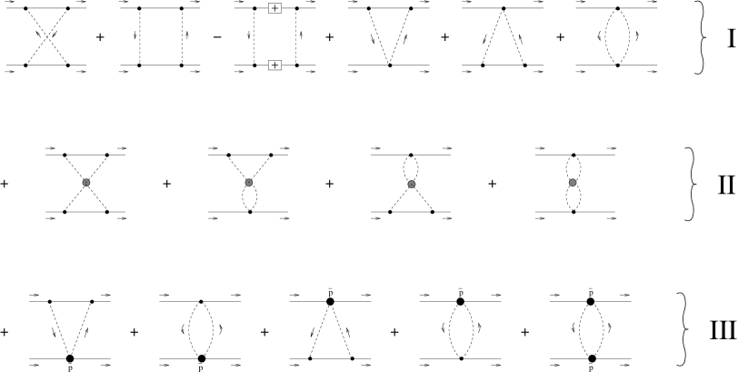
FIG. 2.: Dynamical structure of the TPEP. The first two diagrams of family I correspond to the products of Born $\pi N$ amplitudes, the third one represents the iteration of the OPEP and the next three involve contact interactions associated with the Weinberg-Tomozawa vertex. The diagrams of family II describe medium range effects due to pion-pion correlations. Interactions represented by family III are triangles and bubbles, involving $\pi N$ subthreshold coefficients, indicated by the large black dots.

The dynamical content of the amplitude ${\cal T}_{T\!P}^{(4)}$ is given by the diagrams of Fig. 2. Their full evaluation produces amplitudes containing many different loop integrals, which are interconnected. The chiral orders of the potential are extracted by exploring as much as possible the mathematical relations among the various loop integrals. As the use of these results represents an important step in the determination of the potential, in the Appendix we display their accuracy in configuration space.

The processes given in Fig. 2 are organized into three different families. The first one corresponds to the minimal realization of chiral symmetry [13], includes the subtraction of the iterated OPEP and involves only the pion-nucleon interactions given by ${\cal L}_{N}^{(1)}$, with the constants $m$, $g$ and $f_{\pi}$ used at their physical values. The second family contains two-pion correlations in the $t$ channel, determined by ${\cal L}_{N}^{(1)}$ and ${\cal L}_{\pi}^{(2)}$. Finally, the last family includes chiral corrections representing either higher order processes or other degrees of freedom, hidden into the LECs of ${\cal L}_{N}^{(2)}$ and ${\cal L}_{N}^{(3)}$.

This theoretical structure has been fully incorporated into our recent evaluation of the amplitude ${\cal T}_{T\!P}^{(4)}$, Ref.[25]. In that work we have performed a two-step calculation, using the fact that the $NN$ interaction is closely associated with the off-shell $\pi N$ amplitude. This allows one to use many of the results derived by Becher and Leutwyler [28] (BL) for the $\pi N$ amplitude as inputs into the evaluation of the $NN$ potential. Moreover, it clarifies the relationship between the chiral orders of the $NN$ and $\pi N$ amplitudes. Using Fig. 1, we write the $O(q^{n})$ expansion of ${\cal T}_{T\!P}$ as

$${\cal T}_{T\!P}^{(n)}=-\;\frac{i}{2!}\;\frac{1}{(2\pi)^{4}}\int\left\{\frac{d^{4}Q}{[k^{2}-\mu^{2}]\;[k^{\prime 2}-\mu^{2}]}\right\}\;\sum_{l,m}^{l+m=4}[T_{\pi N}^{(l)}]^{(1)}\;[T_{\pi N}^{(m)}]^{(2)}\;,$$ (2)

where $[T_{\pi N}^{(m)}]^{(i)}$ is the $\pi N$ amplitude for nucleon $(i)$ expanded at order $O(q^{m})$. The factor within curly brackets in the integrand is $O(q^{0})$ whereas the leading term in $T_{\pi N}$, as given by the Weinberg-Tomozawa theorem [33, 34], is $O(q)$. Thus ${\cal T}_{T\!P}^{(n)}$ requires $T_{\pi N}$ up to $O(q^{n-1})$.

This result is important regarding the numerical values of the LECs to be used in the determination of the TPEP, which depend on the chiral order one is working at [35]. These constants are not observables and must be obtained from empirical quantities such as, for instance, $\pi N$ subthreshold coefficients. In the case of our $O(q^{4})$ TPEP, consistency demands the use of LECs determined from $T_{\pi N}$ at $O{(q^{3})}$.

Finally, a further motivation for deriving the TPEP from the intermediate $\pi N$ amplitude is that this stresses the continuity of present developments with the seminal works of the Paris [3] and Stony Brook [4] groups, produced more than three decades ago. For this very reason, one becomes better prepared to understand the specific role played by ChPT in this problem.

III configuration space potential

The configuration space Schrödinger equation is a rather useful tool for calculating low energy nuclear processes. In principle, the $O(q^{4})$ $r$-space potential could be obtained by just performing the Fourier transform of our center of mass $p$-space potential, which is written as

$${t}_{cm}=3\;{t}^{+}+2\;{\mbox{\boldmath$\tau$}}^{(1)}\cdot{\mbox{\boldmath$\tau$}}^{(2)}\;{t}^{-}$$ (3)

with

$${t}_{cm}^{\pm}={t}_{C}^{\pm}+\frac{{\mbox{\boldmath$\Omega$}}_{LS}}{m^{2}}\;{t}_{LS}^{\pm}+\frac{{\mbox{\boldmath$\Omega$}}_{T}}{m^{2}}\;{t}_{T}^{\pm}+\frac{{\mbox{\boldmath$\Omega$}}_{SS}}{m^{2}}\;{t}_{SS}^{\pm}+\frac{{\mbox{\boldmath$\Omega$}}_{Q}}{m^{4}}\;{t}_{Q}^{\pm}\;,$$ (4)

and $\;{\mbox{\boldmath$\Omega$}}_{LS}=i\;({\mbox{\boldmath$\sigma$}}^{(1)}\!+\!{\mbox{\boldmath$\sigma$}}^{(2)})\cdot{\mbox{\boldmath$q$}}\times{\mbox{\boldmath$z$}}/4$, ${\mbox{\boldmath$\Omega$}}_{T}=-{\mbox{\boldmath$q$}}^{2}\;(3{\mbox{\boldmath$\sigma$}}^{(1)}\cdot{\mbox{\boldmath$\hat{q}$}}{\mbox{\boldmath$\sigma$}}^{(2)}\cdot{\mbox{\boldmath$\hat{q}$}}\!-\!{\mbox{\boldmath$\sigma$}}^{(1)}\cdot{\mbox{\boldmath$\sigma$}}^{(2)})$, ${\mbox{\boldmath$\Omega$}}_{SS}={\mbox{\boldmath$q$}}^{2}\;{\mbox{\boldmath$\sigma$}}^{(1)}\cdot{\mbox{\boldmath$\sigma$}}^{(2)}$, and ${\mbox{\boldmath$\Omega$}}_{Q}={\mbox{\boldmath$\sigma$}}^{(1)}\cdot{\mbox{\boldmath$q$}}\!\times\!{\mbox{\boldmath$z$}}\;{\mbox{\boldmath$\sigma$}}^{(2)}\cdot{\mbox{\boldmath$q$}}\!\times\!{\mbox{\boldmath$z$}}$. However, this leads to expressions that contain non-local terms, due to the energy dependence of the profile functions ${t}_{i}$. In order to avoid this kind of complication, we expand the potential in the non-local operators and keep only local and spin-orbit contributions. In this approximation, the configuration space potential becomes

$$V({\mbox{\boldmath$r$}}) = \left(V^{+}_{C}+V^{+}_{LS}\,\Omega_{LS}+V^{+}_{T}\,\Omega_{T}+V^{+}_{SS}\,\Omega_{SS}\right)$$ (5)

$$+ {\mbox{\boldmath$\tau$}}^{(1)}\cdot{\mbox{\boldmath$\tau$}}^{(2)}\left(V^{-}_{C}+V^{-}_{LS}\,\Omega_{LS}+V^{-}_{T}\,\Omega_{T}+V^{-}_{SS}\,\Omega_{SS}\right)$$ (6)

with $\;\Omega_{LS}={\mbox{\boldmath$L$}}\cdot({\mbox{\boldmath$\sigma$}}^{(1)}+{\mbox{\boldmath$\sigma$}}^{(2)})/2,\;\;\Omega_{T}=3\,{\mbox{\boldmath$\sigma$}}^{(1)}\cdot\hat{{\mbox{\boldmath$r$}}}\;{\mbox{\boldmath$\sigma$}}^{(2)}\cdot\hat{{\mbox{\boldmath$r$}}}-{\mbox{\boldmath$\sigma$}}^{(1)}\cdot{\mbox{\boldmath$\sigma$}}^{(2)},\;\;\Omega_{SS}={\mbox{\boldmath$\sigma$}}^{(1)}\cdot{\mbox{\boldmath$\sigma$}}^{(2)}.$

The radial functions are given by

$$V_{C}^{\pm}(r) = \tau^{\pm}\;U_{C}^{\pm}(x)\,,$$ (7)

$$V_{LS}^{\pm}(r) = \tau^{\pm}\;\frac{\mu^{2}}{m^{2}}\,\frac{1}{x}\,\frac{d}{dx}\,U_{LS}^{\pm}(x)\,,$$ (8)

$$V_{T}^{\pm}(r) = \tau^{\pm}\;\frac{\mu^{2}}{m^{2}}\left[\frac{d^{2}}{dx^{2}}-\frac{1}{x}\,\frac{d}{dx}\right]\,U_{T}^{\pm}(x)\,,$$ (9)

$$V_{SS}^{\pm}(r) = -\tau^{\pm}\;\frac{\mu^{2}}{m^{2}}\left[\frac{d^{2}}{dx^{2}}+\frac{2}{x}\,\frac{d}{dx}\right]\,U_{SS}^{\pm}(x)\,,$$ (10)

where $\tau^{+}=3$, $\tau^{-}=2$, $x={\mu}r$, and

$$U^{\pm}_{I}(x)=-\int\frac{d^{3}k}{(2\pi)^{3}}\,e^{i\,{\mbox{\boldmath$k$}}\cdot{\mbox{\boldmath$x$}}}\;{t}^{\pm}_{I}(k)\,,\qquad\qquad I=\{C,LS,T,SS\}$$ (11)

with ${\mbox{\boldmath$k$}}={\mbox{\boldmath$q$}}/\mu$. This allows the potential to be expressed in terms of dimensionless configuration space Feynman integrals, denoted by $S$, and related to the functions $\Pi$ of Ref.[25] by

$$S(x)=\int\frac{d^{3}k}{(2\pi)^{3}}\,e^{i\,{\mbox{\boldmath$k$}}\cdot{\mbox{\boldmath$x$}}}\;\Pi({\mbox{\boldmath$k$}})\,.$$ (12)

Using the results of Sec. IX of Ref.[25], we have the expansions

$$U_{C}^{+}=-\frac{\mu^{3}m^{2}}{256\pi^{2}f_{\pi}^{4}}\;\left[\frac{{\mu}}{m}\right]^{2}\left\{g_{A}^{4}\,(1+4\,\Delta_{GT})\;(1\!-\!{\mbox{\boldmath$\nabla$}}^{2}/2)^{2}\left(S_{\times}-S_{b}\right)\right.$$ (13)

$$\left.+\left[\frac{{\mu}}{m}\right]g_{A}^{2}\;(1\!-\!{\mbox{\boldmath$\nabla$}}^{2}/2)\left[-g_{A}^{2}\left(2S_{a}+{\mbox{\boldmath$\nabla$}}^{2}S_{t}\right)+8\left(\bar{\delta}_{00}^{+}+\bar{\delta}_{01}^{+}{\mbox{\boldmath$\nabla$}}^{2}\right)S_{t}\right]\right.$$ (14)

$$\left.+\left[\frac{{\mu}}{m}\right]^{2}\left[-\frac{m^{2}\,g_{A}^{4}}{16\pi^{2}f_{\pi}^{2}}\;(1\!-\!2{\mbox{\boldmath$\nabla$}}^{2})\left(-4\pi(1\!-\!{\mbox{\boldmath$\nabla$}}^{2}/2)S_{t}+(1\!-\!{\mbox{\boldmath$\nabla$}}^{2}/2)^{2}S_{tt}\right)+\frac{g_{A}^{4}}{4}{\mbox{\boldmath$\nabla$}}^{2}(S_{\times}+S_{b})\right]\right.$$ (15)

$$\left.+\left[\frac{{\mu}}{m}\right]^{2}\left[g_{A}^{4}{\mbox{\boldmath$\nabla$}}^{4}-4g_{A}^{2}\left((\bar{\delta}_{00}^{+}+\bar{\delta}_{01}^{+}{\mbox{\boldmath$\nabla$}}^{2}){\mbox{\boldmath$\nabla$}}^{2}+\delta_{10}^{+}(1-2{\mbox{\boldmath$\nabla$}}^{2}/3+{\mbox{\boldmath$\nabla$}}^{4}/6)\right)\right.\right.$$ (16)

$$\left.\left.+8\left(\bar{\delta}_{00}^{+}+\bar{\delta}_{01}^{+}{\mbox{\boldmath$\nabla$}}^{2}+({\delta}_{10}^{+}/3)(1-{\mbox{\boldmath$\nabla$}}^{2}/4)\right)^{2}+\frac{32}{45}({\delta}_{10}^{+})^{2}(1\!-\!{\mbox{\boldmath$\nabla$}}^{2})^{2}\right]S_{\ell}\right\}\;,$$ (17)

$$U_{LS}^{+}=-\frac{\mu^{3}m^{2}g_{A}^{2}}{128\pi^{2}f_{\pi}^{4}}\;\left[\frac{{\mu}}{m}\right]\left\{g_{A}^{2}\left[(1-{\mbox{\boldmath$\nabla$}}^{2}/2)(\tilde{S}_{b}-S_{t})-(3/2-5{\mbox{\boldmath$\nabla$}}^{2}/8)\,S_{a}\right]\right.$$ (18)

$$\left.+\left[\frac{{\mu}}{m}\right]\left[\frac{g_{A}^{2}}{4}\,(1+2{\mbox{\boldmath$\nabla$}}^{2}-{\mbox{\boldmath$\nabla$}}^{4}/2)\;(S_{\times}+S_{b})+\left(2\,g_{A}^{2}{\mbox{\boldmath$\nabla$}}^{2}-\frac{16}{3}\,\delta^{+}_{10}\,(1\!-\!{\mbox{\boldmath$\nabla$}}^{2}/4)\right)S_{\ell}\right]\right\}\;,$$ (19)

$$U_{T}^{+}=\frac{U_{SS}^{+}}{2}=-\frac{\mu^{3}m^{2}g_{A}^{2}}{768\pi^{2}f_{\pi}^{4}}\;\left\{-g_{A}^{2}\,(1+4\,\Delta{GT})\;(1\!-\!{\mbox{\boldmath$\nabla$}}^{2}/4)\left[S_{\times}+S_{b}\right]\right.$$ (20)

$$\left.-\left[\frac{{\mu}}{m}\right]\frac{g_{A}^{2}}{2}\left[(1-{\mbox{\boldmath$\nabla$}}^{2}/2)(S_{t}-\tilde{S}_{b})+(1-{\mbox{\boldmath$\nabla$}}^{2}/4)S_{a}\right]\right.$$ (21)

$$\left.+\left[\frac{{\mu}}{m}\right]^{2}\left[\frac{g_{A}^{2}}{4}\;(1\!-\!{\mbox{\boldmath$\nabla$}}^{2}/2)^{2}\;S_{\times}+\frac{4}{3}\,\beta^{+}_{00}(1-{\mbox{\boldmath$\nabla$}}^{2}/4)S_{\ell}\right]\right\}\;,$$ (22)

and

$$U_{C}^{-}=-\frac{\mu^{3}m^{2}}{16\pi^{2}f_{\pi}^{4}}\left[\frac{{\mu}}{m}\right]^{2}\left\{\frac{g_{A}^{4}}{16}\,(1+4\,\Delta_{GT})\,(1-{\mbox{\boldmath$\nabla$}}^{2}/2)^{2}(S_{\times}+S_{b})\right.$$ (23)

$$\left.-\frac{1}{4}\left[g_{A}^{4}\,(1+4\,\Delta_{GT})-g_{A}^{2}\,(1+2\,\Delta_{GT})\right](1-{\mbox{\boldmath$\nabla$}}^{2}/2)S_{\ell}\right.$$ (24)

$$\left.+\frac{1}{24}\left[g_{A}^{4}\,(1+4\,\Delta_{GT})-2g_{A}^{2}\,(1+2\,\Delta_{GT})+1\right](1-{\mbox{\boldmath$\nabla$}}^{2}/4)S_{\ell}\right.$$ (25)

$$\left.+\left[\frac{{\mu}}{m}\right]\frac{g_{A}^{2}}{8}(1-{\mbox{\boldmath$\nabla$}}^{2}/2)\left[g_{A}^{2}(S_{a}-{\mbox{\boldmath$\nabla$}}^{2}S_{t}/2)+(g_{A}^{2}-1)(1-{\mbox{\boldmath$\nabla$}}^{2}/2)S_{t}\right]\right.$$ (26)

$$\left.+\left[\frac{{\mu}}{m}\right]^{2}\left\{\frac{g_{A}^{2}}{2}(1-{\mbox{\boldmath$\nabla$}}^{2}/2)\left[-(g_{A}^{2}-1){\mbox{\boldmath$\nabla$}}^{2}/8+\bar{\delta}^{-}_{00}+\bar{\delta}^{-}_{01}{\mbox{\boldmath$\nabla$}}^{2}+\delta^{-}_{10}(1-{\mbox{\boldmath$\nabla$}}^{2}/4)/3+\bar{\beta}^{-}_{00}{\mbox{\boldmath$\nabla$}}^{2}/4\right]\right.\right.$$ (27)

$$\left.\left.-\frac{(g_{A}^{2}-1)}{6}(1-{\mbox{\boldmath$\nabla$}}^{2}/4)\left[\bar{\delta}^{-}_{00}+\bar{\delta}^{-}_{01}{\mbox{\boldmath$\nabla$}}^{2}+3\,\delta^{-}_{10}(1-{\mbox{\boldmath$\nabla$}}^{2}/4)/5+\bar{\beta}^{-}_{00}{\mbox{\boldmath$\nabla$}}^{2}/4\right]\right\}S_{\ell}\right.$$ (28)

$$\left.-\left[\frac{{\mu}}{m}\right]^{2}\frac{m^{2}}{64\pi^{2}f_{\pi}^{2}}\left[\left(2g_{A}^{4}(1-5{\mbox{\boldmath$\nabla$}}^{2}/6+{\mbox{\boldmath$\nabla^{4}$}}/5)+4(g_{A}^{2}-1)^{2}(1-3{\mbox{\boldmath$\nabla$}}^{2}/8+{\mbox{\boldmath$\nabla^{4}$}}/32)/9\right.\right.\right.$$ (29)

$$\left.\left.\left.-4g_{A}^{2}(g_{A}^{2}-1)(1-29{\mbox{\boldmath$\nabla$}}^{2}/72+7{\mbox{\boldmath$\nabla^{4}$}}/144)\right)S_{\ell}\right.\right.$$ (30)

$$\left.\left.\left(g_{A}^{4}(1-{\mbox{\boldmath$\nabla$}}^{2}/2)^{2}-2g_{A}^{2}(g_{A}^{2}-1)(1-{\mbox{\boldmath$\nabla$}}^{2}/2)(1-{\mbox{\boldmath$\nabla$}}^{2}/4)/3+(g_{A}^{2}-1)^{2}(1-{\mbox{\boldmath$\nabla$}}^{2}/4)^{2}\right)S_{\ell\ell}\right]\right.$$ (31)

$$\left.+\left[\frac{{\mu}}{m}\right]^{2}\frac{g_{A}^{4}}{16}(1-{\mbox{\boldmath$\nabla$}}^{2}/2)^{2}({\mbox{\boldmath$\nabla$}}^{2}/4)(S_{\times}-S_{b})\right\}\;,$$ (32)

$$U_{LS}^{-}=-\frac{\mu^{3}m^{2}}{128\pi^{2}f_{\pi}^{4}}\left[\frac{{\mu}}{m}\right]\left\{g_{A}^{4}\left[(3/2-5{\mbox{\boldmath$\nabla$}}^{2}/8)S_{a}-(1-{\mbox{\boldmath$\nabla$}}^{2}/2)(S_{t}+\tilde{S}_{b})\right]\right.$$ (33)

$$\left.+2g_{A}^{2}(g_{A}^{2}-1)(1-{\mbox{\boldmath$\nabla$}}^{2}/4)S_{t}\right.$$ (34)

$$\left.+\left[\frac{{\mu}}{m}\right]\left[(g_{A}^{2}-1)^{2}(1-{\mbox{\boldmath$\nabla$}}^{2}/4)/2+4\,g_{A}^{2}\;\bar{\beta}^{-}_{00}\;(1-{\mbox{\boldmath$\nabla$}}^{2}/2)-4\;(g_{A}^{2}-1)\bar{\beta}^{-}_{00}(1-{\mbox{\boldmath$\nabla$}}^{2}/4)/3\right]S_{\ell}\right.$$ (35)

$$\left.+\left[\frac{{\mu}}{m}\right]\frac{g_{A}^{4}}{4}(1-{\mbox{\boldmath$\nabla$}}^{2}/2)^{2}(S_{\times}-S_{b})\right.$$ (36)

$$\left.-\left[\frac{{\mu}}{m}\right]\frac{m^{2}g_{A}^{4}}{8\pi^{2}f_{\pi}^{2}}\left[-2\pi(1-{\mbox{\boldmath$\nabla$}}^{2}/4)S_{t}+(1-{\mbox{\boldmath$\nabla$}}^{2}/4)^{2}S_{tt}\right]\right\}\;,$$ (37)

$$U_{T}^{-}=\frac{U_{SS}^{-}}{2}=-\frac{\mu^{3}m^{2}}{1536\pi^{2}f_{\pi}^{4}}\;\left[\frac{{\mu}}{m}\right]\left\{g_{A}^{4}\left[(1-{\mbox{\boldmath$\nabla$}}^{2}/2)\,\tilde{S}_{b}+(1-{\mbox{\boldmath$\nabla$}}^{2}/4)\,S_{a}\right]\right.$$ (38)

$$\left.-2\,g_{A}^{2}(g_{A}^{2}-1-2\,\bar{\beta}^{-}_{00})(1-{\mbox{\boldmath$\nabla$}}^{2}/4)\,S_{t}\right.$$ (39)

$$\left.+\left[\frac{{\mu}}{m}\right]\left[-g_{A}^{2}(g_{A}^{2}-1-2\,\bar{\beta}^{-}_{00})(1-{\mbox{\boldmath$\nabla$}}^{2}/2)-(g_{A}^{2}-1-2\,\bar{\beta}^{-}_{00})^{2}(1-{\mbox{\boldmath$\nabla$}}^{2}/4)/3\right]S_{\ell}\right.$$ (40)

$$\left.+\left[\frac{{\mu}}{m}\right]\frac{m^{2}g_{A}^{4}}{8\pi^{2}f_{\pi}^{2}}\left[-2\pi(1-{\mbox{\boldmath$\nabla$}}^{2}/4)S_{t}+(1-{\mbox{\boldmath$\nabla$}}^{2}/4)^{2}S_{tt}\right]\right\}\;,$$ (41)

where the Laplacians act on the variable $x$. The chiral orders of the various radial functions may be read directly from the combination of Eqs. (7)–(10) and (17)–(41). Their relative importances will be discussed in detail in Sec. V. We have expressed our results in terms of the axial coupling $g_{A}$. If one wants, they may be rewritten using the $\pi N$ coupling constant $g$, by means of the relation $g=(1+\Delta_{GT})\,g_{A}\,m/f_{\pi}$, where $\Delta_{GT}$ is the so called Goldberger-Treiman discrepancy.

The parameters $\delta_{ij}^{\pm}$ and $\beta_{ij}^{\pm}$ entering these expressions are determined by subthreshold $\pi N$ coefficients or, alternatively, by the LECs of the effective Lagrangian, according to the results presented in Sec. V of Ref.[25]. Their empirical values are reproduced in Table I.

TABLE I.: Dimensionless subthreshold coefficients; definitions are the same as in Ref.[REFERENCES].

$\bar{\delta}_{00}^{+}$	$\delta_{10}^{+}$	$\bar{\delta}_{01}^{+}$	$\beta_{00}^{+}$
-4.72	3.34	4.15	-10.57
$\bar{\delta}_{00}^{-}$	$\delta_{10}^{-}$	$\bar{\delta}_{01}^{-}$	$\bar{\beta}_{00}^{-}$
7.02	-3.35	-2.05	5.04

The eight functions $S_{i}$ which carry the spatial dependence of the potential are dimensionless and given by

$$S_{\ell} = \frac{K_{1}(2x)}{\pi x^{2}}\;,$$ (42)

$$S_{a} = -\frac{e^{-2x}}{2x^{2}}\;,$$ (43)

$$S_{t} = -\int_{0}^{1}da\int_{0}^{1}db\;\frac{(1-b)\;2m/\mu}{\Lambda_{t}^{2}}\;\frac{e^{-\theta_{t}\,x}}{4\pi x}\;,$$ (46)

$$\Lambda_{t}^{2}=a(1\!-\!a)(1\!-\!b)^{2}\;,$$

$$\theta_{t}^{2}=\left[(1-b)+b^{2}m^{2}/{\mu}^{2}\right]/\Lambda_{t}^{2}\;,$$

$$S_{\times} = \int_{0}^{1}\!db\int_{0}^{1}\!da\;\frac{a^{2}b\;\;\;4m^{2}/{\mu}^{2}}{\Lambda_{\times}^{4}}\;\frac{e^{-{\theta}_{\times}x}}{8\pi{\theta}_{\times}}\;,$$ (49)

$$\Lambda_{\times}^{2}=a(1\!-\!a)(1\!-\!b)\;,$$

$$\theta_{\times}^{2}=\left[(1-ab)+a^{2}b^{2}m^{2}/{\mu}^{2}\right]/\Lambda_{\times}^{2}\;,$$

$$S_{b} = \int_{1}^{\infty}\!dc\int_{0}^{1}\!db\int_{0}^{1}\!da\;\frac{a^{2}b\;\;\;4m^{2}/{\mu}^{2}}{\Lambda_{b}^{4}}\;\frac{e^{-{\theta}_{b}x}}{8\pi{\theta}_{b}}\;,$$ (52)

$$\Lambda_{b}^{2}=a(1-a)(1-b)-a^{2}b^{2}(1-c^{2})/4\;,$$

$$\theta_{b}^{2}=\left[(1-ab)+a^{2}b^{2}c^{2}(m/{\mu})^{2}\right]/\Lambda_{b}^{2}\;,$$

$${\tilde{S}}_{b} = \int_{1}^{\infty}\!dc\int_{0}^{1}\!db\int_{0}^{1}\!da\;\frac{a^{3}b^{2}\;\;\;4m^{3}/{\mu}^{3}}{\Lambda_{b}^{4}}\;\frac{e^{-{\theta}_{b}x}}{8\pi{\theta}_{b}}\;,$$ (53)

$$S_{\ell\ell} = -\frac{1}{4\pi}\int_{0}^{1}da\int_{0}^{1}db\,\frac{\sqrt{(1\!-\!a)(1\!-\!b)}}{(b+a)}\,\frac{1}{x}\,\frac{1}{\left(\frac{1}{a}\!-\!\frac{1}{b}\right)}\left[\left(\frac{4}{a^{2}}\right)^{2}\frac{e^{-2x/a}}{x}\!-\!\left(\frac{4}{b^{2}}\right)^{2}\frac{e^{-2x/b}}{x}\right]\;,$$ (54)

$$S_{tt} = -\frac{(4m\mu)^{2}}{\pi}\int_{0}^{1}da\int_{0}^{1}db\,\frac{G(4\mu^{2}/a)\,G(4\mu^{2}/b)}{a^{2}b^{2}(a+b)}\,\frac{1}{x}\,\frac{1}{\left(\frac{1}{a}\!-\!\frac{1}{b}\right)}\left[e^{-2x/a}\!-\!e^{-2x/b}\right]\;,$$ (55)

where $K_{1}(x)$ is the modified Bessel function and

$$G(t^{\prime})=\frac{2}{m\sqrt{t^{\prime}(4m^{2}-t^{\prime})}}\,\arctan\frac{\sqrt{(4m^{2}-t^{\prime})(t^{\prime}-4\mu^{2})}}{t^{\prime}-2\mu^{2}}\,.$$ (56)

In Figs. 3(a)–3(h) we display the numerical predictions of our TPEP (full line), obtained by using the parameters $\delta_{ij}^{\pm}$ and $\beta_{ij}^{\pm}$ given in table I, fixed by the $\pi N$ subthreshold coefficients of Ref.[22]. As we will discuss in the sequence, our chiral TPEP is theoretically reliable for large distances and definitely not valid for internucleon separations smaller than 1 fm (shaded area). For the sake of producing a feeling for the phenomenological implications of these results, we also plot the medium range components of the Av14 [36] and Av18 [37] versions of the Argonne potential (dotted and dashed lines respectively).

The central isoscalar component of the nuclear force is by far the most important one and the fact that the chiral prediction is consistent with both Argonne versions is rather reassuring. The assessment of the other components is more difficult, since there are important variations between the Av14 and Av18 results. In the cases of $V_{SS}^{+}$, $V_{T}^{-}$, $V_{SS}^{-}$, where these variations do not involve signs, it is possible to note a qualitative agreement with the behavior of the chiral TPEP. The curves for $V_{SS}^{+}$, $V_{C}^{-}$ and $V_{T}^{-}$ are not far from those of Av18 whereas $V_{SS}^{-}$ coincides with the Av14 prediction.

In order to complete the long-distance description of the $NN$ potential, one has to include the OPEP, which contributes only to $V_{T}^{-}$ and $V_{SS}^{-}$, through the following expressions:

$$\left.V_{T}^{-}\right|_{OPEP} = -\frac{m}{E}\,\frac{\mu^{3}g_{A}^{2}}{48\pi m^{2}}\,(1+2\,\Delta_{GT})\left(x^{2}+3x+3\right)\frac{e^{-x}}{x^{3}}\,,$$ (57)

$$\left.V_{SS}^{-}\right|_{OPEP} = \frac{m}{E}\,\frac{\mu^{3}g_{A}^{2}}{48\pi m^{2}}\,(1+2\,\Delta_{GT})\,\frac{e^{-x}}{x}\,.$$ (58)

These components, which dominate at large distances, are shown in Figs. 4.(a) and 4.(b), together with the corresponding TPEP contributions. The influence of the TPEP only becomes significant in $V_{T}^{-}$ for $r<$ 2 fm, and in $V_{SS}^{-}$, for $r<$ 3 fm.

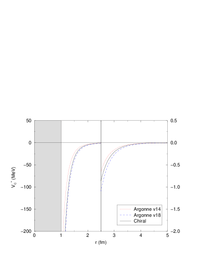
FIG. 3(a).: Central isoescalar component.

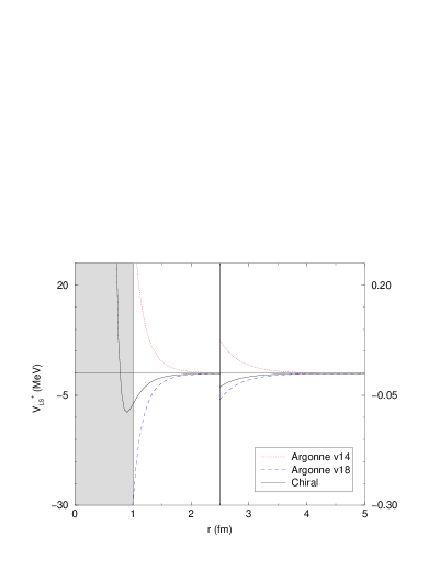
FIG. 3(b).: Spin-orbit isoescalar component.

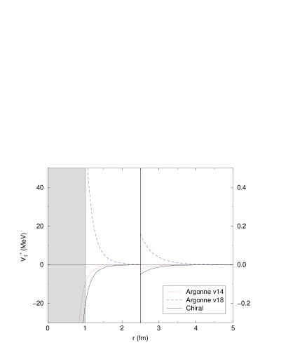
FIG. 3(c).: Tensor isoescalar component.

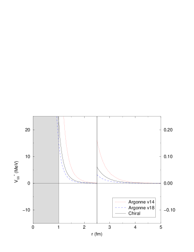
FIG. 3(d).: Spin-spin isoescalar component.

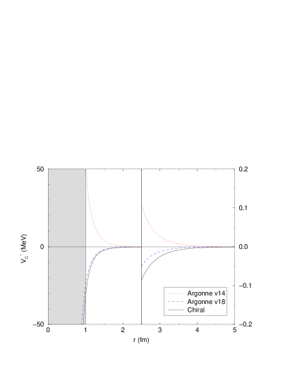
FIG. 3(e).: Central isovector component.

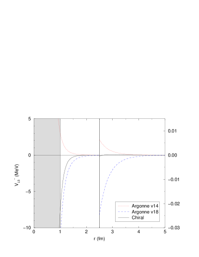
FIG. 3(f).: Spin-orbit isovector component.

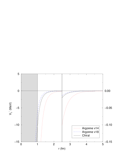
FIG. 3(g).: Tensor isovector component.

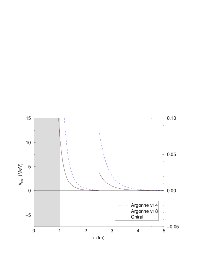
FIG. 3(h).: Spin-spin isovector component.

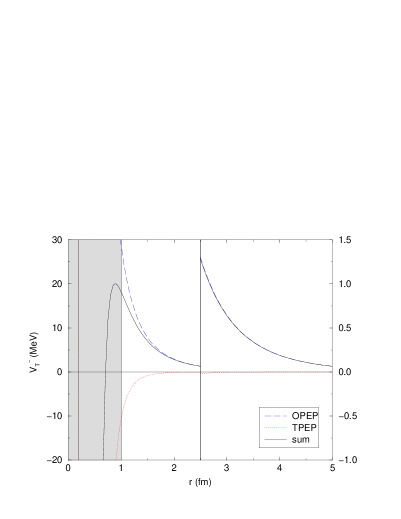
FIG. 4.(a).: OPEP and TPEP contributions to the tensor isovector potential.

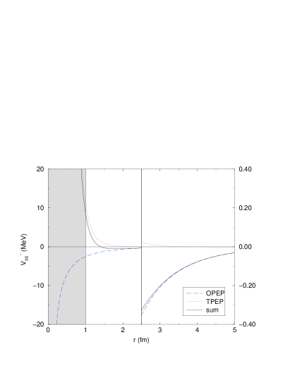
FIG. 4.(b).: OPEP and TPEP contributions to the spin-spin isovector potential.

IV internal dynamics

In this section we discuss the relative importance of the contributions originating from the three families of diagrams presented in Fig. 2. This is motivated by the fact that the chiral description of the TPEP consists of a well defined field theoretical structure which depends on external parameters representing masses ($\mu$, $m$), coupling constants ($f_{\pi}$, $g_{A}$), and LECs ($c_{i}$, $d_{i}$). In order to be able to obtain predictions, one has to feed the mathematical structure with the empirical values of these parameters.

The constants present in the $O(q^{4})$ potential may be divided into two classes, according to their numerical accuracy. The values of $\mu$, $m$, $f_{\pi}$, and $g_{A}$ entering ${\cal L}_{\pi}^{(2)}$ and ${\cal L}_{N}^{(1)}$ may be considered as being very precise for the purposes of determining the TPEP. On the other hand, the constants $c_{i}$ and $d_{i}$ that appear in ${\cal L}_{N}^{(2)}$ and ${\cal L}_{N}^{(3)}$ need to be extracted from $\pi N$ subthreshold coefficients by means of dispersion relations and hence may contain both experimental and theoretical uncertainties. This means that, in the case of the interactions given in Fig. 2, predictions from families I and II are very reliable whereas those associated with family III may be less so. For this reason it is important to establish how the results discussed in the preceding section depend on the various families of diagrams.

In order to assess the importance of each family we show, in Fig. 5, their relative contributions to the components of the TPEP. A general pattern one can observe is that two-loop contributions (family II) are negligible and, in particular, exactly zero for $V_{LS}^{+}$, $V_{SS}^{+}$, and $V_{T}^{+}$. The various profile functions are neatly dominated by either family I or III. The former, which is very precise, dominates the channels $V_{C}^{-}$, $V_{LS}^{+}$, $V_{SS}^{+}$, and $V_{T}^{+}$ and a modification on the values of the LECs would hardly influence the corresponding curves. This can be viewed as a strong constraint on the construction of phenomenological potentials. For the remaining channels, this condition is somehow relaxed, since they are dominated by the diagrams of family III. If one wishes, the freedom in these channels may be used to fix experimentally the LECs by means of $NN$ data.

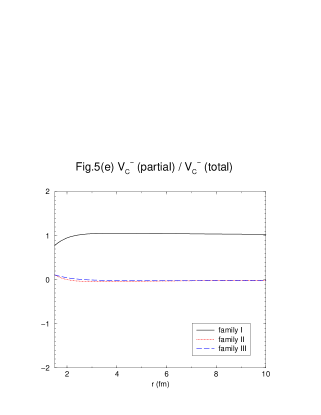
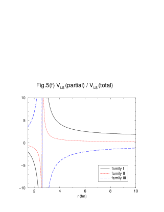
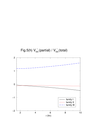
FIG. 5.: Relative weight of each family in the TPEP, obtained by dividing the partial contributions by the full result.

V chiral structure

In this section, we discuss chiral scales. In the case of the central components, these scales can be read directly from the functions $U^{\pm}_{C}$, given by Eqs. (17) and (32). For the other terms, there is a factor $(\mu^{2}/m^{2})$ in the relation between $V^{\pm}$ and $U^{\pm}$, arising from the non-relativistic expansion of the Dirac spinors, (8)–(10). Thus, in the $O(q^{4})$ potential, one expands the corresponding functions $U^{\pm}$ up to $O(q^{2})$.

The leading term of the chiral TPEP is $O(q^{2})$ and our results are written as sums of $O(q^{2})$, $O(q^{3})$, and $O(q^{4})$ contributions. In the cases of $V_{T}^{+}$, $V_{SS}^{+}$, and $V_{C}^{-}$, this structure is mapped directly into the corresponding profile functions. The other components begin at $O(q^{3})$.

In $p$-space, the chiral series involves nucleon three-momenta, assumed to be small. This means that, in $r$-space, the chiral structure should become apparent at large distances. In order to check this, in Fig. 6 we show the ratios of the chiral layers for the various components of the potential. In all figures it is possible to note, at large distances, a rather well defined chiral hierarchy. Corrections are always smaller than the terms they correct. On the other hand, this hierarchy tends to break down when distances decrease and we assume that our results are not physical for $r<$ 1 fm. In two cases, namely, $V_{C}^{+}$ and $V_{LS}^{-}$, corrections are large within the region of physical interest.

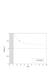
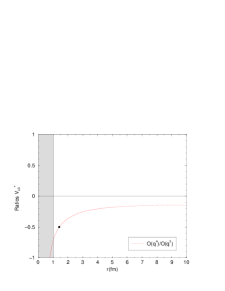
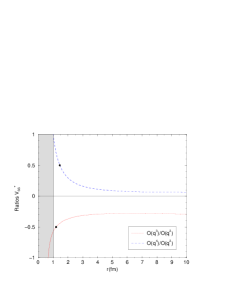
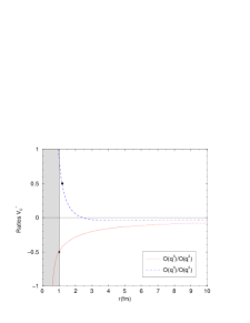
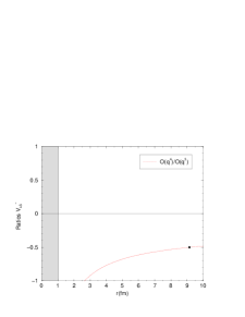
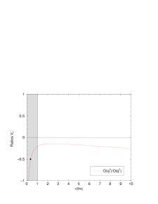
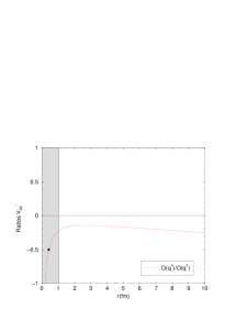
FIG. 6.: Relative contribution of each chiral order to the TPEP. The point in the curve where the ratio is 0.5 is indicated by a black dot, for the sake of guiding the eye.

VI the heavy baryon approximation

The relativistic potential is expressed by Eqs. (7)–(10), (17)–(41), and involves eight basic functions, denoted generically by $S(x)$. They are given by Eqs. (42)–(55), and represent bubble, triangle, crossed box, planar box, double bubble, and double triangle diagrams. These functions have been derived by means of covariant techniques and correspond to the signature of relativity in this problem. Only the bubble integral can be evaluated analytically and the other ones are not homogeneous functions of either the pion mass or external three-momenta. In general, the expansion of the functions $S(x)$ in powers of $q/m$ is not mathematically defined. However, as discussed by Ellis and Tang [29], if one forces such an expansion, one recovers formally the results of HBChPT. In Ref.[25] we have expanded our $O(q^{4})$ $p$-space relativistic potential in this way and obtained (inequivalent) expressions that reproduce most of the standard $O(q^{4})$ HBChPT results [17, 20, 21, 24]. Differences are due to the Goldberger-Treiman discrepancy and to the procedure adopted for subtracting the iterated OPEP. In this section, we discuss the numerical implications of the heavy baryon approximation in configuration space.

We begin by considering the triangle integral $S_{t}$, given by Eq. (46), that can also be expressed as [27]

$$S_{t}=-\frac{8m}{\mu}\int_{4\mu^{2}}^{\infty}dt^{\prime}\;\mbox{Im}\gamma(t^{\prime})\;\frac{e^{-\sqrt{t^{\prime}/\mu^{2}}\,x}}{x}$$ (59)

with

$$\mbox{Im}\;\gamma(t^{\prime})=\frac{1}{8\pi\sqrt{t^{\prime}(4m^{2}-t^{\prime})}}\,\arctan\left[\frac{\sqrt{(4m^{2}-t^{\prime})(t^{\prime}-4\mu^{2})}}{t^{\prime}-2\mu^{2}}\right]\,.$$ (60)

The heavy baryon approximation consists in writing

$$\mbox{Im}\;\gamma(t^{\prime})\simeq\frac{1}{16\pi m\sqrt{t^{\prime}}}\,\arctan\left[\frac{2m\sqrt{t^{\prime}-4\mu^{2}}}{t^{\prime}-2\mu^{2}}\right]$$ (61)

and treating formally the argument

$$\alpha=\frac{2m\sqrt{t^{\prime}-4\mu^{2}}}{t^{\prime}-2\mu^{2}}$$ (62)

as being $O(q^{-1})$. This would suggest that one could use the result $\arctan\alpha=\pi/2-1/\alpha+1/3\alpha^{3}+\cdots$ in order to derive the heavy baryon expansion of the triangle integral. Recently BL [27] have discussed the properties of the spectral representation based on Eq. (62) and remarked that the series for $\arctan$ which underlies the heavy baryon approximation is valid only in the domain $|\alpha|\geq 1$. For $|\alpha|<1$ one should use $\arctan\alpha=\alpha-\alpha^{3}/3+\cdots$, but this corresponds to an expansion in inverse powers of $q$. They showed that a suitable representation for $S_{t}$ is

$$S_{t}^{B\!L} = -\frac{8m}{\mu}\int_{4\mu^{2}}^{\infty}dt^{\prime}\;\frac{e^{-\sqrt{t^{\prime}/\mu^{2}}\,x}}{x}\;\frac{1}{16\pi m\sqrt{t^{\prime}}}\,\arctan\left[\frac{2m\sqrt{t^{\prime}-4\mu^{2}}}{t^{\prime}-2\mu^{2}}\right]$$ (63)

$$\approx -\frac{1}{2\pi m\mu}\int_{4\mu^{2}}^{\infty}dt^{\prime}\;\frac{1}{\sqrt{t^{\prime}}}\left\{\left[\frac{\pi}{2}-\frac{(t^{\prime}-2\mu^{2})}{2m\sqrt{t^{\prime}\!-\!4\mu^{2}}}\right]_{\!HB}\right.$$ (64)

$$+ \left.\left[\frac{\mu\sqrt{t^{\prime}}}{2m\sqrt{t^{\prime}\!-\!4\mu^{2}}}-\frac{\sqrt{t^{\prime}}}{2\mu}\arctan\frac{\mu^{2}}{m\sqrt{t^{\prime}\!-\!4\mu^{2}}}\right]_{\!t\!h}\right\}\;\frac{e^{-\sqrt{t^{\prime}/\mu^{2}}\,x}}{x}\;.$$ (65)

The heavy baryon approximation consists in keeping only the first bracket in the integrand. However, this does not cover the region $t^{\prime}\sim 4\mu^{2}$, where the second term dominates. As a consequence, the heavy baryon approximation of $S_{t}$, which reads

$$S_{t}\rightarrow S_{t}^{H\!B}=\left[-\;\frac{e^{-2x}}{2x^{2}}\right]^{LO}+\left[\frac{\mu}{2m}\frac{2}{\pi x^{2}}\;[xK_{0}(2x)+K_{1}(2x)]+\right]^{NLO}\cdots\;,$$ (66)

is not suitable for all values of $x$, as observed numerically in our previous work [38]. The exponential in the integrand of Eq. (59) shows clearly that, for large values of $x$, results are dominated by the lower end of the integration. Thus, a good description of $S_{t}$ at large distances requires a decent representation for $\mbox{Im}\;\gamma(t^{\prime})$ near $t^{\prime}=4\mu^{2}$.

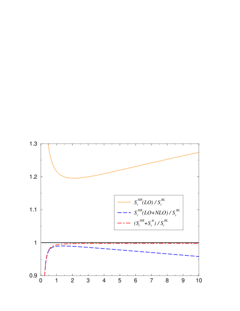
FIG. 7.: The heavy baryon expansion of the triangle integral, given by Eq. (66), and the relativistic BL correction ($S_{t}^{th}$), divided by $S_{t}^{BL}$.

In Fig. 7 we display the ratios of the various terms of Eq. (65) by Eq. (63). Inspecting this figure one learns that the first two terms of the heavy baryon series do not represent well the full result. In order to have a good description of $S_{t}^{BL}$ at large distances one has to add $S_{t}^{th}$ which, as pointed out by BL, cannot be obtained through the heavy baryon series.

An advantage of the heavy baryon formalism is that it gives rise to power counting, which is absent in relativistic baryon ChPT based on dimensional regularization [9]. In order to overcome this difficulty, BL proposed a new regularization scheme, based on a previous work by Ellis and Tang [29]. The so called Infrared Regularization (IR) respects the correct analytic structure around the point $t^{\prime}=4\mu^{2}$, is manifestly Lorentz invariant, and gives rise to power counting.

In the case of the triangle integral, the infrared regularized expressions reads

$$S_{t}^{I\!R} = -\int_{0}^{1}da\int_{0}^{\infty}db\;\frac{(1-b)\;2m/\mu}{\Lambda_{t}^{2}}\;\frac{e^{-\theta_{t}\,x}}{4\pi x}$$ (67)

with $\Lambda_{t}^{2}$ and $\theta_{t}$ given by Eq. (46).

In Fig. 8 we compare the infrared regularized triangle integral ($S_{t}^{I\!R}$) with that given by Eq. (46), obtained through dimensional regularization. For comparison, we also plot the results of the heavy baryon formulation at $LO$ and $NLO$. The relativistic versions of the triangle integral are numerically identical for $r>$ 1.5 fm, indicating that the form of the regularization procedure is irrelevant in the region of physical interest.

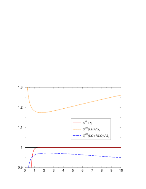
FIG. 8.: The heavy baryon approximation of the triangle integral.

The discussion about the triangle integral may be extended to the functions $S_{\times}$, $S_{b}$, and $\tilde{S}_{b}$, associated with crossed box and planar box diagrams, and given by Eqs. (49)–(53). The heavy baryon approximations for these results read [25]

$$S_{\times}^{H\!B} \cong \frac{2}{\pi x}\,K_{0}(2x)\!-\!\left[\frac{\mu}{m}\right]\frac{e^{-2x}}{2x}\!-\!\left[\frac{\mu}{m}\right]^{2}\left\{\frac{1}{\pi x^{2}}\left[2xK_{0}(2x)+(1\!-\!x^{2})K_{1}(2x)\right]\right\}\!+\!\cdots\;,$$ (68)

$$S_{b}^{H\!B} \cong \frac{2}{\pi x}\,K_{0}(2x)\!-\!\left[\frac{\mu}{m}\right]\frac{e^{-2x}}{4x}\!-\!\left[\frac{\mu}{m}\right]^{2}\left\{\frac{1}{3\pi x^{2}}\left[2xK_{0}(2x)+(1\!-\!x^{2})K_{1}(2x)\right]\right\}\!+\!\cdots\;,$$ (69)

$$\tilde{S}_{b}^{H\!B} \cong \frac{e^{-2x}}{4x^{2}}\!-\!\left[\frac{\mu}{m}\right]\frac{2}{3\pi x^{2}}\left[xK_{0}(2x)+K_{1}(2x)\right]\!+\!\left[\frac{\mu}{m}\right]^{2}\frac{3\;e^{-2x}}{32x}\!+\!\cdots\;.$$ (70)

The quality of these heavy baryon approximations may be assessed in Figs. 9–11, where the partial sums are divided by the relativistic result, Eqs. (49)–(53).

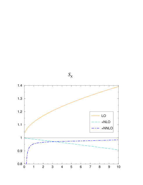
FIG. 9.: The heavy baryon approximation of $S_{\times}$. The partial sums are divided by the relativistic result, Eq. (49).

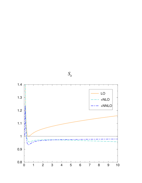
FIG. 10.: The heavy baryon approximation of $S_{b}$. The partial sums are divided by the relativistic result, Eq. (52).

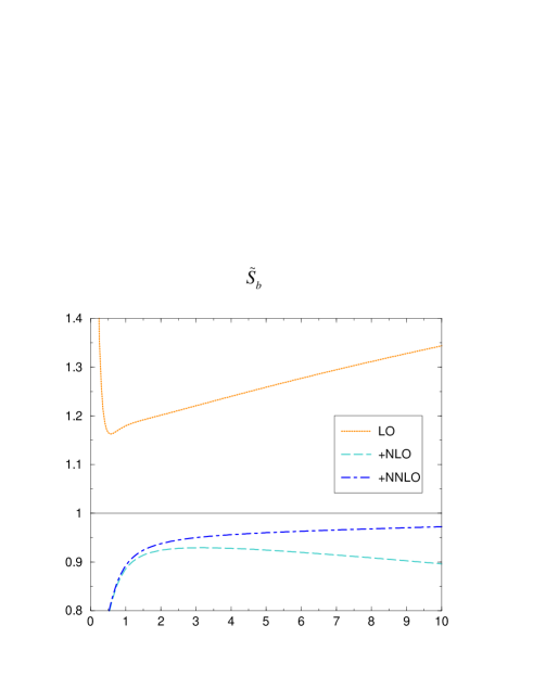
FIG. 11.: The heavy baryon approximation of $\tilde{S}_{b}$. The partial sums are divided by the relativistic result, Eq. (53).

VII conclusions

In this work we have studied the main features, in configuration space, of a relativistic $O(q^{4})$ expansion of the two-pion exchange nucleon-nucleon potential derived recently by ourselves [25]. Chiral symmetry provides a mathematical structure for the potential, that has to be fed with numerical values for $\mu$, $m$, $f_{\pi}$, $g_{A}$, and the LECs $c_{i}$ and $d_{i}$. The main source of uncertainty are the values of those LECs, which need to be extracted from $\pi N$ scattering data.

The profile functions for the various non relativistic components of the potential were compared with two phenomenological versions produced by the Argonne group. One finds good agreement with their central scalar term, which dominates the $NN$ interaction. In all cases in which the signs of the Argonne potentials coincide, there is a qualitative agreement with our results.

In order to check how empirical uncertainties can affect numerical results, we have studied the dynamical content of the potential in terms of families of diagrams associated with either the $[{\cal L}_{\pi}^{(2)}+{\cal L}_{N}^{(1)}]$ or $[{\cal L}_{N}^{(2)}+{\cal L}_{N}^{(3)}]$ pieces of the effective Lagrangian. In all but one cases, dynamics is clearly dominated by one of these interactions. In particular, $V_{LS}^{+}$, $V_{T}^{+}$, $V_{SS}^{+}$, and $V_{C}^{-}$ are dominated by $[{\cal L}_{\pi}^{(2)}+{\cal L}_{N}^{(1)}]$ and hence fixed by the values of $g_{A}$ and $f_{\pi}$ only. The components $V_{C}^{+}$, $V_{T}^{-}$, and $V_{SS}^{-}$, on the other hand, are dominated by $[{\cal L}_{N}^{(2)}+{\cal L}_{N}^{(3)}]$ and their numerical values may be affected by the less certain LECs $c_{i}$ and $d_{i}$.

Most components of the potential are given as sums of $O(q^{2})$, $O(q^{3})$, and $O(q^{4})$ terms. The relative weights of these terms of the chiral series have been investigated and one finds good convergence at large distances. However, there are two cases, namely, $V_{C}^{+}$ and $V_{LS}^{-}$, where convergence is not evident in the region of physical interest. We intend to deal with this problem elsewhere.

Finally, the relationship between relativistic and heavy baryon results has been discussed. On the purely conceptual side, the view seems to be well accepted nowadays that they cannot be fully equivalent. This is indeed the case and the numerical implications of this statement in configuration space were found to be of the order of 5%.

Several chiral calculations of the TPEP were produced in the last decade. As we pointed out in the introduction we expect, in the spirit of effective theories of QCD, that all these calculations should eventually converge to a single result.

It is in this conceptual framework that we discuss here the relationship between the present work and its earlier versions, published between 1994 and 1997 [13, 16]. In Ref.[25], the $O(q^{4})$ expansion of the TPEP was performed in three steps. In step 1, we derived full amplitudes, by using standard covariant techniques, to evaluate the diagrams of Fig. 2. At this stage, results were quite similar to those of Ref.[16], although not identical, as we discuss in the sequence. A handicap of the full amplitudes is that they involve several cancellations and do not exhibit chiral scales explicitly. Therefore, in step 2 we derived intermediate results, that show these scales, by just rewriting the full amplitudes with the help of exact relations among Feynman integrals. We subsequently neglected short distance terms and, in that region, full and intermediate results became no longer identical. The transmogrification of the potential was based on the following relations:

Relation 01: $$\bar{S}_{cc}^{(000)}=\frac{1}{3}\left(1-{\mbox{\boldmath$\nabla$}}^{2}/{4}\right){S}_{cc}^{(000)}+\cdots\;,$$ (71)

Relation 02: $$\bar{\bar{S}}_{cc}^{(000)}=\frac{1}{15}\left(1-{\mbox{\boldmath$\nabla$}}^{2}/{4}\right)^{2}{S}_{cc}^{(000)}+\cdots\;,$$ (72)

Relation 03: $$\left[1-(\mu/m)^{2}\,{\mbox{\boldmath$\nabla$}}^{2}/{4}\right]{S}_{sc}^{(001)}={S}_{cc}^{(000)}-\frac{\mu}{2m}\left(1-{\mbox{\boldmath$\nabla$}}^{2}/{2}\right){S}_{sc}^{(000)}+\cdots\;,$$ (73)

Relation 04: $$\left[1-(\mu/m)^{2}\,{\mbox{\boldmath$\nabla$}}^{2}/{4}\right]{S}_{sc}^{(002)}+\bar{S}_{sc}^{(000)}=-\frac{\mu}{2m}\left(1-{\mbox{\boldmath$\nabla$}}^{2}/{2}\right){S}_{sc}^{(001)}+\cdots\;,$$ (74)

Relation 05: $$\bar{S}_{sc}^{(000)}=\frac{1}{2}\left(1-{\mbox{\boldmath$\nabla$}}^{2}/{4}\right){S}_{sc}^{(000)}+\frac{\mu}{4m}\left(1-{\mbox{\boldmath$\nabla$}}^{2}/{2}\right){S}_{sc}^{(001)}+\cdots\;,$$ (75)

Relation 06: $$\left[1-(\mu/m)^{2}\,{\mbox{\boldmath$\nabla$}}^{2}/{4}\right]{S}_{ss}^{(001)}={S}_{sc}^{(000)}-\frac{\mu}{2m}\left(1-{\mbox{\boldmath$\nabla$}}^{2}/{2}\right){S}_{ss}^{(000)}+\cdots\;,$$ (76)

Relation 07: $$\bar{S}_{ss}^{(000)}=-{S}_{sc}^{(001)}+\cdots\;,$$ (77)

Relation 08: $$\left[1-(\mu/m)^{2}\,{\mbox{\boldmath$\nabla$}}^{2}/{4}\right]{S}_{ss}^{(002)}+\bar{S}_{ss}^{(000)}={S}_{sc}^{(001)}-\frac{\mu}{2m}\left(1-{\mbox{\boldmath$\nabla$}}^{2}/{2}\right){S}_{ss}^{(001)}+\cdots\;,$$ (78)

Relation 09: $$\left[1-(\mu/m)^{2}\,{\mbox{\boldmath$\nabla$}}^{2}/{4}\right]^{2}{S}_{ss}^{(002)}+\left[1-(\mu/m)^{2}\,{\mbox{\boldmath$\nabla$}}^{2}/{4}\right]\bar{S}_{ss}^{(000)}=\frac{\mu^{2}}{4m^{2}}\left(1-{\mbox{\boldmath$\nabla$}}^{2}/{2}\right)^{2}\;{S}_{ss}^{(000)}$$ (80)

$$+\left[1-(\mu/m)^{2}\,{\mbox{\boldmath$\nabla$}}^{2}/{4}\right]{S}_{sc}^{(001)}-\frac{\mu}{2m}\left(1-{\mbox{\boldmath$\nabla$}}^{2}/{2}\right){S}_{sc}^{(000)}+\cdots\;,$$

Relation 10: $$\bar{S}_{ss}^{(000)}=\left(1-{\mbox{\boldmath$\nabla$}}^{2}/{4}\right){S}_{ss}^{(000)}+\frac{\mu}{2m}\left(1-{\mbox{\boldmath$\nabla$}}^{2}/{2}\right){S}_{ss}^{(001)}+\cdots\;,$$ (81)

Relation 11: $$-{S}_{sc}^{(000)}=+\frac{\mu}{2m}\left(1-{\mbox{\boldmath$\nabla$}}^{2}/{2}\right){S}_{reg}^{(000)}-\frac{1}{\sqrt{1-(\mu/m)^{2}\,{\mbox{\boldmath$\nabla$}}^{2}/{4}}}\,{S}_{a}+\cdots\;,$$ (82)

Relation 12: $$\left[1-(\mu/m)^{2}\,{\mbox{\boldmath$\nabla$}}^{2}/{4}\right]{S}_{reg}^{(002)}+\bar{S}_{reg}^{(000)}={S}_{sc}^{(001)}+\cdots\;,$$ (83)

Relation 13: $$\bar{S}_{reg}^{(000)}=-{S}_{sc}^{(001)}+\frac{\mu}{2m}\left(1-{\mbox{\boldmath$\nabla$}}^{2}/{2}\right){S}_{reg}^{(010)}+\cdots\;,$$ (84)

Relation 14: $$-\frac{\mu^{2}}{4m^{2}}\left(1-{\mbox{\boldmath$\nabla$}}^{2}/{2}\right)^{2}\;{S}_{reg}^{(000)}=$$ (86)

$$\frac{\mu}{2m}\left(1-{\mbox{\boldmath$\nabla$}}^{2}/{2}\right){S}_{sc}^{(000)}-\frac{\mu}{2m}\left(1-{\mbox{\boldmath$\nabla$}}^{2}/{2}\right)\,\frac{1}{\sqrt{1-(\mu/m)^{2}\,{\mbox{\boldmath$\nabla$}}^{2}/{4}}}\,{S}_{b}^{(000)}+\cdots\;,$$

Relation 15: $$\bar{S}_{reg}^{(000)}=\left(1-{\mbox{\boldmath$\nabla$}}^{2}/{4}\right){S}_{reg}^{(000)}-\frac{\mu}{2m}\left(1-{\mbox{\boldmath$\nabla$}}^{2}/{2}\right){S}_{reg}^{(010)}+\cdots\;.$$ (87)

In these expressions, the ellipses indicate short range terms, which have been neglected. In order to produce a feeling for the accuracy of these approximations, in table II we display the quantity $\Delta_{i}(r)=|1-R_{i}(r)/L_{i}(r)|$, where $L_{i}(r)$ $R_{i}(r)$ are respectively the values of the left and right hand sides of relation $i$ at point $r$. Inspection of this table shows that, although discrepancies may be large at short distances, in all cases they remain below 1% for $r\geq 1.5$ fm.

TABLE II.: Approximations made in relations among integrals.

	$r=0.1$ fm	$r=0.5$ fm	$r=1.0$ fm	$r=1.5$ fm
Rel. 01	0.000019	0.000000	0.000000	0.000000
Rel. 02	0.000004	0.000000	0.000000	0.000000
Rel. 03	0.004272	0.000001	0.000000	0.000000
Rel. 04	0.000433	0.000000	0.000000	0.000000
Rel. 05	0.002478	0.000001	0.000000	0.000000
Rel. 06	0.056091	0.000002	0.000000	0.000000
Rel. 07	0.000000	0.000000	0.000000	0.000000
Rel. 08	0.005502	0.000010	0.000000	0.000000
Rel. 09	0.271267	0.000347	0.000000	0.000000
Rel. 10	0.034881	0.000009	0.000000	0.000000
Rel. 11	0.958301	0.096190	0.000076	0.000312
Rel. 12	0.000096	0.000030	0.000001	0.000000
Rel. 13	0.855452	0.134455	0.006010	0.000168
Rel. 14	1.007437	1.105614	0.066393	0.006432
Rel. 15	1.554767	0.417655	0.018483	0.000513

Finally, in step 3, we obtain the $O(q^{4})$ expansion of the TPEP, given in section III, by truncating the results of step 2 at that order.

We now compare the results of this work with those from earlier versions. Our 1994 paper [13] dealt with the evaluation of the diagrams given in family I of Fig.2, which corresponds to the minimal realization of chiral symmetry in the TPEP. The main differences with our present results concern second order corrections, due to the way variable $W$, representing the total CM energy, was approximated in the planar box diagram. In 1994 paper we used $W=2m$, following Partovi and Lomon [31]. We no longer perform this crude approximation.

In our 1997 paper [16] we have calculated the diagrams shown in family III of Fig.2 and results can be directly related with those of the present work, provided one establishes the connection between the two notations. For instance, the central isoscalar potential was formerly written as

$$\left.V^{+}_{C}\right|_{III} = -\frac{\mu}{4\pi}\frac{3}{2}\left\{g^{2}\frac{\mu}{m}\alpha_{mn}^{+}\left[2S_{B(2m,n)}+2S^{V}_{T(2m,n)}\right]+\alpha^{+}_{k\ell}\alpha^{+}_{mn}S_{B(2k+2m,\ell+n)}\right.$$ (88)

$$+ g^{2}\frac{\mu}{m}\beta_{mn}^{+}\left[2S^{V}_{B(2m+1,n)}+2S^{W}_{T(2m+1,n)}\right]+\alpha^{+}_{k\ell}\beta^{+}_{mn}S^{V}_{B(2k+2m+1,\ell+n)}$$ (89)

$$+ \left.\beta^{+}_{k\ell}\beta^{+}_{mn}S^{W}_{B(2k+2m+2,\ell+n)}+g^{2}\frac{\mu}{m}\beta_{mn}^{+}\,2S^{g}_{T(2m+1,n)}+\beta^{+}_{k\ell}\beta^{+}_{mn}S^{q}_{B(2k+2m+2,\ell+n)}\right\}\;,$$ (90)

where $S$ are Feynman integrals from Ref.[16] and $\alpha_{mn}^{+}$ and $\beta_{mn}^{+}$ are linear combinations of $\pi N$ subthreshold coefficients. In order to recast the old results in the form adopted in this work, one may use the relations

$$S_{B(0,n)} = \frac{(-1)^{n}}{4\pi}\left(1-{\mbox{\boldmath$\nabla$}}^{2}/4\right)^{n}\;S_{cc}^{000}$$ (91)

$$S_{B(2,n)} = S^{g}_{B(0,n)}=S^{V}_{B(1,n)}=\frac{(-1)^{n}}{4\pi}\left(1-{\mbox{\boldmath$\nabla$}}^{2}/4\right)^{n}\;\bar{S}_{cc}^{000}$$ (92)

$$S_{B(4,n)} = 3S^{g}_{B(2,n)}=S^{V}_{B(3,n)}=(3/2)S^{W}_{B(2,n)}=\frac{(-1)^{n}}{4\pi}\left(1-{\mbox{\boldmath$\nabla$}}^{2}/4\right)^{n}\;\bar{\bar{S}}_{cc}^{000}$$ (93)

$$S^{V}_{T(0,n)} = \frac{(-1)^{n}}{4\pi}\left(1-{\mbox{\boldmath$\nabla$}}^{2}/4\right)^{n}\;(-)S_{sc}^{001}$$ (94)

$$S^{V}_{T(2,n)} = S^{W}_{T(1,n)}+S^{g}_{T(1,n)}$$ (95)

$$S^{W}_{T(1,n)} = \frac{(-1)^{n}}{4\pi}\left(1-{\mbox{\boldmath$\nabla$}}^{2}/4\right)^{n}\;(-)\left[S_{sc}^{003}+2\bar{S}_{sc}^{001}\right]$$ (96)

$$S^{g}_{T(1,n)} = -\frac{(-1)^{n}}{4\pi}\left(1-{\mbox{\boldmath$\nabla$}}^{2}/4\right)^{n}\;(-)\bar{S}_{sc}^{001}$$ (97)

The parameters $\alpha^{+}_{mn}$ and $\beta^{+}_{mn}$ are related to subthreshold coefficients by

$$\alpha_{00}^{+} = \mu\left(\bar{d}_{00}^{+}+4\mu^{2}\bar{d}_{01}^{+}+16\mu^{4}\bar{d}_{02}^{+}\right)$$ (98)

$$\alpha_{01}^{+} = 4\mu^{3}\left(\bar{d}_{01}^{+}+8\mu^{2}\bar{d}_{02}^{+}\right)$$ (99)

$$\alpha_{02}^{+} = 16\mu^{5}\left(\bar{d}_{02}^{+}\right)$$ (100)

$$\alpha_{10}^{+} = \mu^{3}\left[\bar{d}_{10}^{+}-{b}_{00}^{+}+4\mu^{2}(\bar{d}_{11}^{+}-b_{01}^{+})\right]$$ (101)

$$\alpha_{11}^{+} = 4\mu^{5}\left(\bar{d}_{11}^{+}-{b}_{01}^{+}\right)$$ (102)

$$\beta_{00}^{+} = \mu^{3}\left({b}_{00}^{+}+4\mu^{2}{b}_{01}^{+}+16\mu^{4}{b}_{02}^{+}\right)$$ (103)

$$\beta_{01}^{+} = 4\mu^{5}\left({b}_{01}^{+}+8\mu^{2}{b}_{02}^{+}\right)$$ (104)

$$\beta_{02}^{+} = 16\mu^{7}\left({b}_{02}^{+}\right)$$ (105)

Just as an example, using these rules in the case of the triangle contribution to Eq. (90) and truncating at $O(q^{4})$, we find

$$V_{C}^{+}\left.\right|_{III}^{t} = -\frac{\mu}{4\pi}\frac{3}{2}g^{2}\frac{\mu}{m}2\left[\alpha_{0n}^{+}S^{V}_{T(0,n)}+\alpha_{1n}^{+}S^{V}_{T(2,n)}+\beta_{0n}^{+}\left(S^{W}_{T(1,n)}+S^{g}_{T(1,n)}\right)\right]$$ (106)

$$= +3[\mu]\left(\frac{g}{4\pi}\right)^{2}\frac{\mu}{m}\left[\left(\bar{d}_{00}^{+}+\bar{d}_{01}^{+}t+\bar{d}_{02}^{+}t^{2}\right)S_{sc}^{001}+\left(\bar{d}_{10}^{+}+\bar{d}_{11}^{+}t\right)\left(S_{sc}^{003}+3\bar{S}_{sc}^{001}\right)\right]\,.$$ (107)

We have recently checked explicitly all the results of our 1997 paper and found out that they are equivalent with those of the present work if we make the approximation $W=2m$.

There are still two important sources of differences between these two sets of results. The first one is due to the fact that those of the earlier work were not truncated at a given order. The second one is that it did not include explicitly the two-loop diagrams, as we do now. In 1997 these effects were hidden within the $\pi N$ sub-threshold coefficients and were therefore double counted. Even if these effects are numerically small, as we discussed in section IV of this work, this represents a rather important conceptual difference between both calculations. As two-loop contributions only arise at $O(q^{4})$, the potential produced in 1997 would be numerically identical with the present one for distances larger than 1.5 fm if both of them were truncated at $O(q^{3})$.

REFERENCES

• [1] M. Taketani, S. Nakamura, and M. Sasaki, Prog. Theor. Phys. VI, 581 (1951).
• [2] M. Taketani, S. Machida, and S. Ohnuma, Prog. Theor. Phys. 7, 45 (1952); A. Klein, Phys. Rev. 91, 740 (1953); K. A. Brueckner and K. M. Wilson, ibid. 92, 1023 (1953).
• [3] W.N. Cottingham and R. Vinh Mau, Phys.Rev. 130, 735 (1963); W.N. Cottingham, M. Lacombe, B. Loiseau, J.M. Richard, and R. Vinh Mau, Phys.Rev. D 8, 800 (1973); M. Lacombe, B. Loiseau, J. M. Richard, R. Vinh Mau, J. CotΓ©, P. Pires, and R. de Tourreil, Phys. Rev. C 21, 861 (1980).
• [4] G. E. Brown and J. W. Durso, Phys. Lett. 35B, 120 (1971); M. Chemtob, J. W. Durso, and D. O. Riska, Nucl. Phys. B38, 141 (1972).
• [5] S. A. Coon, M. D. Scadron, P. C. McNamee, B. R. Barrett, D. W. E. Blatt, and B. H. J. McKellar, Nucl. Phys. A317, 242 (1979).
• [6] M. R. Robilotta and C. Wilkin, J. Phys. G 4, L115 (1978).
• [7] S. Weinberg, Physica A 96, 327 (1979).
• [8] J . Gasser and H. Leutwyler, Ann. Phys. (N.Y.) 158, 142 (1984).
• [9] J. Gasser, M.E.Sainio, and A.Ε varc, Nucl. Phys. B307, 779 (1988).
• [10] S. Weinberg, Phys. Lett. B 251, 288 (1990); Nucl. Phys. B363, 3 (1991).
• [11] C. OrdΓ³Γ±ez and U. van Kolck, Phys. Lett. B 291, 459 (1992).
• [12] L.S. Celenza, A. Pantziris, and C.M. Shakin, Phys.Rev. C 46, 2213 (1992); J.L. Friar and S.A. Coon, ibid. 49, 1272 (1994); M.C. Birse, ibid. 49,2212 (1994).
• [13] C.A. da Rocha and M.R. Robilotta, Phys.Rev. C 49, 1818 (1994).
• [14] C. OrdΓ³Γ±ez, L. Ray, and U. van Kolck, Phys. Rev. Lett. 72, 1982 (1994); Phys.Rev. C 53, 2086 (1996); N. Kaiser, S. GerstendΓΆrfer, and W. Weise, Nucl.Phys. A637, 395 (1998).
• [15] R.Tarrach and M.Ericson, Nucl.Phys. A294, 417 (1978); M. R. Robilotta, Nucl.Phys. A595, 171 (1995).
• [16] M. R. Robilotta and C.A.da Rocha, Nucl. Phys. A615,391 (1997).
• [17] N. Kaiser, R. Brockman, and W. Weise, Nucl. Phys. A625, 758 (1997).
• [18] M.C.M. Rentmeester, R.G.E. Timmermans, J.L. Friar, and J.J. de Swart, Phys. Rev. Lett. 82, 4992 (1999); M.C.M. Rentmeester, R.G.E. Timmermans, and J.J. de Swart, Phys. Rev. C 67, 044001 (2003).
• [19] E. Epelbaum, W. GlΓΆckle, and Ulf-G. Meissner, Nucl. Phys. A637, 107 (1998); Nucl. Phys. A671, 295 (2000).
• [20] N. Kaiser, Phys. Rev. C 64, 057001 (2001).
• [21] N. Kaiser, Phys. Rev. C 65, 017001 (2001).
• [22] G. HΓΆhler, in Numerical Data and Functional Relationships in Science and Technology, edited by H.Schopper, Landolt-BΓΆrnstein, New Series, Group I, Vol. 9, Subvol. b, Pt. 2 (Springer-Verlag, Berlin, 1983); G.HΓΆhler, H.P.Jacob, and R.Strauss, Nucl.Phys. B39, 273 (1972).
• [23] J-L.Ballot, C.A.da Rocha, and M.R.Robilotta, Phys.Rev. C 57, 1574 (1998).
• [24] D.R. Entem and R. Machleidt, Phys. Rev. C 66, 014002 (2002).
• [25] R. Higa and M.R. Robilotta, Phys. Rev. C 68, 024004 (2003).
• [26] N. Fettes and U-G. Meissner, Nucl. Phys. A679, 629 (2001); N. Fettes and U-G. Meissner, Nucl. Phys. A640, 199 (1998).
• [27] T. Becher and H. Leutwyler, Eur. Phys. J. C 9, 643 (1999).
• [28] T. Becher and H. Leutwyler, J. High Energy Phys. 106, 17 (2001).
• [29] H.-B. Tang, hep-ph/9607436, P.J. Ellis and H.-B. Tang, Phys. Rev. C 57, 3356 (1998); K. Torikoshi and P. Ellis, Phys.Rev. C 67, 015208 (2003).
• [30] U-G. Meissner, At the Frontier of Particle Physics: Handbook of QCD, edited by M. Shifman, (World Scientific, Singapore, 2001) Vol.1, p.417.
• [31] M. H. Partovi and E. Lomon, Phys. Rev. D 2, 1999 (1970).
• [32] D.R. Entem and R. Machleidt, preprint nucl-th/0303017 (2003).
• [33] S. Weinberg, Phys. Rev. Lett. 17, 616 (1966).
• [34] Y. Tomozawa, Nuovo Cimento A 46, 707 (1966).
• [35] M. MojΕΎiΕ‘ and J. Kambor, Phys. Lett. B 476, 344 (2000).
• [36] R.B. Wiringa, R.A. Smith, and T.L. Ainsworth, Phys. Rev. C 29, 1207 (1984).
• [37] R. B. Wiringa, V. G. J. Stoks, and R. Schiavilla, Phys. Rev. C 51, 38 (1995).
• [38] M. R. Robilotta, Phys. Rev. C 63, 044004 (2001).