Hartree-Fock-Bogoliubov Calculations in Coordinate Space:
Neutron-Rich Sulfur, Zirconium, Cerium, and Samarium Isotopes

Abstract

Using the Hartree-Fock-Bogoliubov (HFB) mean field theory in coordinate space, we investigate ground state properties of the sulfur isotopes from the line of stability up to the two-neutron dripline (${}^{34-52}S$). In particular, we calculate two-neutron separation energies, quadrupole moments, and rms-radii for protons and neutrons. Evidence for shape coexistence is found in the very neutron-rich sulfur isotopes. We compare our calculations with results from relativistic mean field theory and with available experimental data. We also study the properties of neutron-rich zirconium (${}^{102,104}Zr$), cerium (${}^{152}Ce$), and samarium (${}^{158,160}Sm$) isotopes which exhibit very large prolate quadrupole deformations.

I Introduction

One of the fundamental questions of nuclear structure physics is: how many neutrons or protons can we add to a given nuclear isotope before it becomes unstable against spontaneous nucleon emission? The neutron-rich side of the nuclear chart, in particular, exhibits thousands of nuclear isotopes still to be explored with new Radioactive Ion Beam facilities DOE02 . Another limit to stability is the superheavy element region around $Z=124-126$ and $N=184$ which is formed by a delicate balance between strong Coulomb repulsion and additional binding due to closed shells KB00 . Theoretically, one expects profound differences between the known isotopes near stability and exotic nuclei at the neutron dripline, e.g. the appearance of neutron halos and neutron skins, and large pairing correlations.

There are various theoretical approaches to the nuclear many-body problem. For the lightest nuclei, e.g. ${}^{12}C$, an exact diagonalization of the Hamiltonian in a shell model basis is feasible NV00 ; NO02 . Stochastic methods like the shell model Monte Carlo approach KDL97 ; PD03 may be used for medium-mass nuclei up to $A\sim 60$. For heavier nuclei, theorists tend to utilize self-consistent mean field theories; both non-relativistic versions WS94 ; DN96 ; TH96 ; CB98 ; RD99 ; SD00 ; YM01 ; TOU03 and relativistic versions Ri96 ; LR99 ; KB00 have been developed. As long as the pairing interaction is relatively weak, it is permissible to treat the mean field and the pairing field separately via Hartree-Fock theory with added BCS or Lipkin/Nogami pairing. This works well near the line of stability WS94 . However, as one approaches the driplines, pairing correlations increase dramatically and it is essential to treat both the mean field and the pairing field selfconsistently within the Hartree-Fock-Bogoliubov (HFB) formalism YM01 . While the HF(B) theories describe the ground state properties of nuclei, their excited states can be obtained with the (quasiparticle) random phase approximation (Q)RPA Ma01 ; BD02 ; IJ03 .

In this paper we study the ground state properties of neutron-rich even-even nuclei up to the two-neutron dripline. Besides the large pairing correlations already mentioned, HFB calculations face another problem in this region: not only does one have to consider “well-bound” single-particle states (which determine the structure near stability), but in addition there are occupied “weakly-bound” states with large spatial extent. Furthermore, because the Fermi energy for neutrons $\epsilon_{F}\approx 0$ at the dripline, virtual excitations into the continuum states become important for a proper description of the HFB ground state. All of these features represent major challenges for the numerical solution.

Traditionally, the HFB equations have been solved by expanding the quasiparticle wavefunctions in a harmonic oscillator basis ER93 . This works very well near the line of $\beta-$ stability because only “well-bound” states need to be considered. However, as one approaches the driplines, the numerical solution becomes more challenging: in practice, it is very difficult to represent continuum states as superpositions of bound harmonic oscillator states because the former show oscillatory behavior at large distances while the latter decay exponentially. On the other hand, a direct solution of the HF(B) equations on a finite-size coordinate space lattice does not suffer from the above-mentioned shortcomings because no region of the spatial lattice is favored over any other region: well-bound, weakly- bound and (discretized) continuum states can be represented with the same accuracy. Therefore, the spatial lattice representation has inherent advantages for the theoretical description of exotic nuclei.

Using our recently developed HFB lattice code for deformed nuclei far from stability TOU03 , we have investigated the ground state properties of the sulfur isotope chain, starting at the line of stability ($N=16$) up to the two-neutron dripline (which turns out to be $N=36$ in our HFB calculations). Our calculations show both spherical and quadrupole- deformed g.s. deformations; in addition, there is evidence for shape coexistence in the very neutron-rich region. In particular, we calculate two-neutron separation energies, quadrupole moments, and rms-radii for protons and neutrons. Our HFB calculations are compared with results from relativistic mean field theory and with available experimental data.

We have also carried out HFB calculations for some recently measured heavier systems: among medium and heavy nuclei, ¹⁰⁴Zr ($\beta_{2}=0.45(4)$) and ¹⁵⁸Sm ($\beta_{2}=0.46(5)$) are among the most deformed isotopes HR03 . The large deformation could have its origin in the high spin down-sloping orbitals near $Z=38,40,62$ and $N=40,64,96$. These large prolate deformations at ¹⁰⁴Zr and ¹⁵⁸Sm are confirmed by Hartree-Fock-Bogoliubov calculations carried out in the present work.

II HFB equations in coordinate space

Recently, we have solved for the first time the HFB continuum problem in coordinate space for deformed nuclei in two spatial dimensions without any approximations, using Basis-Spline methods TOU03 . The novel feature of our HFB code is that it is capable of generating high-energy continuum states with an equivalent single-particle energy of hundreds of MeV. In fact, early 1-D calculations for spherical nuclei DN96 and our recent 2-D HFB calculations have demonstrated that one needs continuum states with an equivalent single-particle energy up to 60 MeV to describe the ground state properties accurately near the neutron dripline. Moreover, recent QRPA calculations by Terasaki et al. Te03 suggest that one needs to consider continuum states up to $150$ MeV for the description of collective excited states. It should be mentioned that current 3-D HFB codes in coordinate space, e.g. Ref. TH96 ; YM01 , utilize an expansion of the quasiparticle wavefunctions in a truncated HF-basis which is limited to continuum states up to about $5$ MeV of excitation energy. Alternatively, an expansion in a stretched oscillator basis has also been explored SD00 .

A detailed description of our theoretical method has been published in ref. TOU03 ; in the following, we give a brief summary. In coordinate space representation, the HFB Hamiltonian and the quasiparticle wavefunctions depend on the distance vector ${\bf r}$, spin projection $\sigma=\pm\frac{1}{2}$, and isospin projection $q=\pm\frac{1}{2}$ (corresponding to protons and neutrons, respectively). In the HFB formalism, there are two types of quasiparticle wavefunctions, $\phi_{1}$ and $\phi_{2}$, which are bi-spinors of the form

$$\phi^{q}_{1,\alpha}({\bf r})=\left(\begin{array}[]{c}\phi^{q}_{1,\alpha}({\bf r,\uparrow})\\ \phi^{q}_{1,\alpha}({\bf r,\downarrow})\end{array}\right),\ \ \phi^{q}_{2,\alpha}({\bf r})=\left(\begin{array}[]{c}\phi^{q}_{2,\alpha}({\bf r,\uparrow})\\ \phi^{q}_{2,\alpha}({\bf r,\downarrow})\end{array}\right).$$ (1)

The quasiparticle wavefunctions determine the normal density $\rho_{q}({\bf r})$ and the pairing density $\tilde{\rho}_{q}({\bf r})$ as follows

$$\rho_{q}({\bf r})\ = \ \sum_{E_{\alpha}>0}^{\infty}\sum_{\sigma=-\frac{1}{2}}^{+\frac{1}{2}}\phi^{q}_{2,\alpha}({\bf r}\sigma)\ \phi^{q\ *}_{2,\alpha}({\bf r}\sigma)\ ,$$ (2)

$$\tilde{\rho_{q}}({\bf r})\ = \ -\sum_{E_{\alpha}>0}^{\infty}\sum_{\sigma=-\frac{1}{2}}^{+\frac{1}{2}}\phi^{q}_{2,\alpha}({\bf r}\sigma)\ \phi^{q\ *}_{1,\alpha}({\bf r}\sigma)\ .$$ (3)

In the wavefunctions, the dependence on the quasiparticle energy $E_{\alpha}$ is denoted by the index $\alpha$ for simplicity.

In the present work, we use Skyrme effective N-N interactions in the p-h channel, and a delta interactions in the p-p channel. For these types of effective interactions, the particle mean field Hamiltonian $h$ and the pairing field Hamiltonian $\tilde{h}$ are diagonal in isospin space and local in position space,

$$h({\bf r}\sigma q,{\bf r}^{\prime}\sigma^{\prime}q^{\prime})\ =\ \delta_{q,q^{\prime}}\ \delta({\bf r}-{\bf r}^{\prime})h^{q}_{\sigma,\sigma^{\prime}}({\bf r})$$ (4)

and

$$\tilde{h}({\bf r}\sigma q,{\bf r}^{\prime}\sigma^{\prime}q^{\prime})\ =\ \delta_{q,q^{\prime}}\ \delta({\bf r}-{\bf r}^{\prime})\tilde{h}^{q}_{\sigma,\sigma^{\prime}}({\bf r})\ .$$ (5)

and the HFB equations have the following structure in spin-space TOU03 :

$$\left(\begin{array}[]{cc}(h^{q}-\lambda)&\tilde{h}^{q}\\ \tilde{h}^{q}&-(h^{q}-\lambda)\end{array}\right)\left(\begin{array}[]{c}\phi^{q}_{1,\alpha}\\ \phi^{q}_{2,\alpha}\end{array}\right)=E_{\alpha}\left(\begin{array}[]{c}\phi^{q}_{1,\alpha}\\ \phi^{q}_{2,\alpha}\end{array}\right)$$ (6)

with

$$h^{q}({\bf r})=\left(\begin{array}[]{cc}h^{q}_{\uparrow\uparrow}({\bf r})&h^{q}_{\uparrow\downarrow}({\bf r})\\ h^{q}_{\downarrow\uparrow}({\bf r})&h^{q}_{\downarrow\downarrow}({\bf r})\end{array}\right),\ \tilde{h}^{q}({\bf r})=\left(\begin{array}[]{cc}\tilde{h}^{q}_{\uparrow\uparrow}({\bf r})&\tilde{h}^{q}_{\uparrow\downarrow}({\bf r})\\ \tilde{h}^{q}_{\downarrow\uparrow}({\bf r})&\tilde{h}^{q}_{\downarrow\downarrow}({\bf r})\end{array}\right)\ \ .$$ (7)

The quasiparticle energy spectrum is discrete for $|E|<-\lambda$ and continuous for $|E|>-\lambda$ DN96 . For even-even nuclei it is customary to solve the HFB equations for positive quasiparticle energies and consider all negative energy states as occupied in the HFB ground state.

III Numerical method

Using cylindrical coordinates $(r,z,\phi)$, we introduce a 2-D grid $(r_{\alpha},z_{\beta})$ with $\alpha=1,...,N_{r}$ and $\beta=1,...,N_{z}$. In radial direction, the grid spans the region from $0$ to $r_{max}$. Because we want to be able to treat octupole shapes, we do not assume left-right symmetry in $z$-direction. Consequently, the grid extends from $-z_{max}$ to $+z_{max}$. Typically, $z_{max}\approx r_{max}$ and $N_{z}$ $\approx$ $2\cdot N_{r}$.

For the lattice representation, the wavefunctions and operators are represented in terms of Basis-Splines. B-Splines of order $M$, $B^{M}_{i}(x)$, are a set ($i=1,...,{\cal N}$) of piecewise continuous polynomial sections of order $M-1$; a special case are the well-known finite elements which are B-Splines of order $M=2$. By using B-Splines of seventh or ninth oder, we are able to represent derivative operators very accurately on a relatively coarse grid with a lattice spacing of about 0.8 fm resulting in a lattice Hamiltonian matrix of relatively low dimension. While our current 2-D lattices are linear, a major advantage of the B-Spline technique is that it can be extended to nonlinear lattices (e.g. exponentially increasing) KO96 which will be particularly useful for problems where one is interested in the behavior of wavefunctions at very large distances.

The four components ($n=1,...,4$) of the HFB bi-spinor wavefunction $\psi_{n}(r,z)$ are expanded in terms of a product of B-Splines

$$\psi_{n}(r_{\alpha},z_{\beta})=\sum_{i=1}^{{\cal N}_{i}}\sum_{j=1}^{{\cal N}_{j}}B^{M}_{i}(r_{\alpha})B^{M}_{j}(z_{\beta})c^{ij}_{n}\ .$$ (8)

We construct the derivative operators contained in the Hamiltonian with the B-Spline Galerkin method OU99 while local potentials are represented by the collocation method WO95 ; KO96 . The numerical solution of the HFB equations results in a set of quasiparticle wavefunctions at the lattice points. The corresponding quasiparticle energy spectrum contains both bound and (discretized) continuum states. We diagonalize the HFB Hamiltonian separately for fixed isospin projection $q$ and angular momentum projection $\Omega$. Note that the number of quasiparticle eigenstates is determined by the dimensionality of the lattice HFB Hamiltonian. For fixed values of $q$ and $\Omega$, we obtain $4\cdot N_{r}\cdot N_{z}$ eigenstates, typically up to 1,000 MeV.

In ref.TOU03 ; UOT03 we have investigated the numerical convergence of several observables as a function of lattice box size, grid spacing, and maximum angular momentum projection $\Omega_{max}$. In the case of spherical nuclei, our calculations have been compared with the 1-D radial HFB results of Dobaczewski et al. DN96 , and indeed there is good agreement between the two. Production runs of our HFB code are carried out on an IBM-SP massively parallel supercomputer using OPENMP/MPI message passing. Parallelization is possible for different angular momentum states $\Omega$ and isospins (p/n).

IV Numerical results and comparison with experimental data

In this section we present numerical results of our 2D-HFB code and compare these to experimental data and other theoretical methods. In all of our calculations we utilized the Skyrme (SLy4) CB98 effective N-N interaction in the p-h and h-p channel, and for the p-p and h-h channel we use a delta interaction with the same parameter set as in ref. TOU03 : a pairing strength of $V_{0}=-170.0\;MeVfm^{3}$, with an equivalent s.p. energy cutoff parameter ${\cal E}_{max}=60$ MeV. All calculations reported in this paper were carried out with B-Spline order $M=7$ and maximum angular momentum projection $\Omega_{max}=\frac{21}{2}$.

IV.1 Sulfur isotope chain up to the two-neutron dripline; shape coexistence studies

The sulfur isotopes ($Z=16$) have been investigated several years ago by Werner et al. WS94 using self-consistent mean field models: both Skyrme-HF and relativistic mean field (RMF) model calculations were carried out using a simple heuristic “constant pairing gap” approximation. Because of the well-known deficiencies of standard pairing theory in the exotic neutron-rich region, we have decided to re-investigate the sulfur isotope chain, starting at the line of stability ($N=16$) up to the two-neutron dripline (which turns out to be $N=36$ in our HFB calculations). Based on the above-mentioned earlier calculations, one may expect a wide range of ground state deformations, and in addition there has been some evidence for shape coexistence in this region WS94 . Because our HFB code TOU03 has been specifically designed to describe deformed exotic nuclei, the sulfur isotopes are expected to provide a rich testing ground for our calculations.

Within the single-particle shell model, one would expect nuclei such as ${}^{44}_{16}S_{28}$ with “magic” neutron number $N=28$ to be spherical. But the mean field theories predict, in fact, deformed intrinsic shapes as a result of “intruder” states. Furthermore, in some of these isotopes shape coexistence has been predicted WS94 . All these phenomena depend strongly on the interplay between the mean field and the pairing field with is correctly described the the HFB theory. Furthermore, the neutron-rich $N\approx 28$ nuclei play a crucial role in astrophysics for the nucleosynthesis of the heavy Ca-Ti-Cr isotopes S93 .

In radial ($r$) direction, our lattice extends from $0-12$ fm, and in symmetry axis ($z$) direction from $-12,...,+12$ fm, with a lattice spacing of about $0.8$ fm in the central region. Angular momentum projections $\Omega=1/2,3/2,...,21/2$ were taken into account.

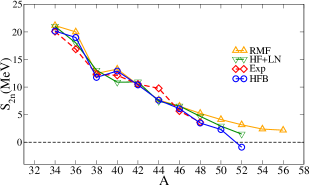
Figure 1: Two-neutron separation energies for sulfur isotopes. The dripline is located where the separation energy becomes zero.

Figure 1 shows the calculated two-neutron separation energies for the sulfur isotope chain. The two-neutron separation energy is defined as

$$S_{2n}(Z,N)\ =\ E_{bind}(Z,N)\ -\ E_{bind}(Z,N-2)\;.$$ (9)

Note that in using this equation, all binding energies must be entered with a positive sign. The position of the two-neutron dripline is defined by the condition $S_{2n}(Z,N)\ =0$, and nuclei with negative two-neutron separation energy are unstable against the emission of two neutrons.

The two-neutron separation energies have been calculated using various methods: in addition to HFB calculations (i.e. selfconsistent mean field with pairing), we have also carried out Hartree-Fock calculations with added Lipkin/Nogami pairing (HF+LN), and we compare our results to the relativistic mean field with BCS pairing (RMF) calculations by Lalazissis et al. LR99 . Experimental data based on measured binding energies AW95 are available up to the isotope ${}^{48}S$. Fig. 1 shows that both the HFB and RMF calculations are in good agreement with experiment where available but there are dramatic differences as we approach the two-neutron dripline: Our HFB calculations predict ${}^{50}S$ to be the last isotope that is stable against the emission of two neutrons. By contrast, the RMF approach predicts $S_{2n}(Z,N)>0$ at least up to ${}^{56}S$. Our HF+LN calculations also yield positive $2n$-separation energies in the mass region investigated here. It should be stressed that, on theoretical grounds, neither BCS-type nor Lipkin-Nogami type pairing is justified for the very neutron-rich isotopes. Furthermore, it is well-known that the HF+LN method breaks down at magic numbers (the pairing gap does not vanish).

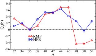
Figure 2: Quadrupole moment for protons (in units of barn) for even-even sulfur isotopes.

In Fig. 2 we show a comparison of the HFB and RMF results for the intrinsic electric quadrupole moments of the sulfur isotopes. In most cases, the HFB and RMF calculations show a similar trend: we observe a region with predominantly prolate deformation. Note, however, that for the most neutron-rich sulfur isotopes, our HFB theory predicts a prolate ground state whereas RMF theory yields an oblate shape. Direct measurements of electric quadrupole moments are only available for two of the sulfur isotopes. The data compilation of Stone S01 yields intrinsic electric quadrupole moments of $Q^{exp}=-0.15b$ for ${}^{32}S$ and $Q^{exp}=+0.04b$ for ${}^{34}S$. Our HFB code yields $Q_{HFB}=+0.113b$ and $+0.203b$ for these two isotopes. The RMF calculations of Lalazissis et al. LR99 give values of $Q_{RMF}=+0.339b$ and $+0.159b$, respectively.

In intermediate-energy Coulomb excitation experiments, the energies and $B(E2)$ values of the lowest excited $2^{+}$ state were measured for ${}^{38,40,42}S$ Sch96 and for ${}^{44}S$ Gl97 . The analysis of the measured $BE(2)$ values in terms of the simple quadrupole-deformed rotor model yields the following experimental quadrupole deformations for the even sulfur isotopes ${}^{38-44}S$: $|\beta_{2}^{exp}|=0.246(16),\ 0.284(16),\ 0.300(24),\ 0.258(36)$; our corresponding Skyrme-HFB theory results are $\beta_{2}^{HFB}=0.16,\ 0.26,\ 0.25,\ 0.29$. Apparently, the HFB results for ${}^{40,42,44}S$ are in good agreement with experiment, but there is a discrepancy in the case of ${}^{38}S$: Skyrme-HFB predicts a less deformed shape than the experimental value. There is an even larger discrepancy between experiment and the RMF calculations which yield an almost spherical shape, $\beta_{2}^{RMF}=0.054$.

Both HFB and RMF calculations reveal shape coexistence in this region, with an energy difference between the ground state and the shape isomer that is usually quite small. For example, in the case of ${}^{48}_{16}S_{32}$ our HFB code yields a ground state binding energy of $-362.56$ MeV with a quadrupole deformation of $\beta_{2}=0.11$, and an oblate minimum at $\beta_{2}=-0.15$ which is only $0.49$ MeV higher than the ground state. The RMF predicts in this case a ground state binding energy of $-362.97$ MeV with oblate deformation of $\beta_{2}=-0.25$, and a shape isomer with $\beta_{2}=+0.179$ which is located $0.29$ MeV above the ground state.

In Fig. 3 we show a comparison of the quadrupole moment for neutrons predicted by our HFB calculations and the RMF results of ref.LR99 . In both cases, the general trend is very similar to the result obtained for protons.

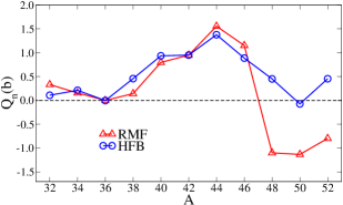
Figure 3: Quadrupole moment for neutrons (in units of barn) for even-even sulfur isotopes.

In Fig. 4 we compare the root-mean-square radii of protons and neutrons predicted by our HFB calculations and the RMF calculations with BCS pairing LR99 . Near the line of $\beta$-stability, the proton and neutron radii are almost identical, but as we approach the $2n$-dripline, we see clearly the development of a “neutron skin” as evidenced by the large difference between the neutron and proton rms radii. For example, in ${}^{50}_{16}S_{34}$ our HFB calculations yield $r_{n}=3.935$ fm and $r_{p}=3.364$ fm, respectively. In general, the RMF calculations predict larger neutron rms radii for mass numbers $A\geq 38$ than do our HFB calculations.

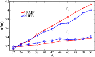
Figure 4: Root mean square radii of protons and neutrons for even-even sulfur isotopes.

IV.2 Strongly deformed neutron-rich zirconium, cerium, neodymium, and samarium isotopes

Recently, triple-gamma coincidence experiments have been carried out with Gammasphere at LBNL HR03 which have determined half-lives and quadrupole deformations of several neutron-rich zirconium, cerium, and samarium isotopes. Furthermore, laser spectroscopy measurements Ca02 for zirconium isotopes have yielded precise rms-radii in this region. These medium/heavy mass nuclei are among the most neutron-rich isotopes ($N/Z\approx 1.6$) for which spectroscopic data are available. It is therefore of great interest to compare these data with the predictions of the selfconsistent HFB mean field theory.

A comparison of our HFB results and experimental data is given in table 1. The theoretical quadrupole deformations of the proton charge distributions agree very well with the measured data of ref.HR03 . In addition, our calculated proton rms-radius for ${}^{102}Zr$ is in good agreement with recent laser spectroscopic measurements (see Fig.4 of ref.Ca02 ). Theoretical HFB predictions are also given for the neutron density distributions.

Table 1: Our HFB results for neutron-rich zirconium, cerium, neodymium, and samarium isotopes. The first column lists the neutron-to-proton ratio $N/Z$. Subsequent columns display quadrupole deformations $\beta_{2}(p),\beta_{2}(n)$ and rms-radii $r_{p},r_{n}$ of protons and neutrons. Recent experimental data for quadrupole deformations are taken from ref.HR03 . The rms-radius for ${}^{102}Zr$ was measured in ref.Ca02 .

	$N/Z$	$\beta_{2}(p)$	$\beta_{2}^{exp}(p)$	$\beta_{2}(n)$	$r_{p}$ (fm)	$r_{p}^{exp}$ (fm)	$r_{n}$ (fm)
${}^{102}Zr$	1.55	0.43	0.42(5)	0.43	4.47	4.54	4.65
${}^{104}Zr$	1.60	0.45	0.45(4)	0.45	4.49		4.70
${}^{152}Ce$	1.62	0.32	0.30(3)	0.33	5.01		5.22
${}^{156}Nd$	1.60	0.37		0.36	5.08		5.27
${}^{160}Sm$	1.58	0.38		0.37	5.13		5.31

In table 2 we give a more detailed comparison of various theoretical calculations for ${}^{158}_{\ 62}Sm$. As stated earlier, only the HFB theory provides a self-consistent treatment of both mean field and pairing properties. In contrast, the HF + Lipkin/Nogami and the RMF calculations treat mean field and pairing as separate entities. By comparing the HFB and HF+LN results in the first two columns with the measured binding energies and quadrupole deformations (last column) we find that our HFB lattice calculation yields values which are closer to the experimental data. Table 2 also shows that while the RMF theory reproduces the experimental binding energy quite well it seriously underpredicts the strong quadrupole deformation measured in ref. HR03 . In addition, table 2 compares theoretical results for other observables such as rms-radii for neutrons and protons, Fermi energies ($\lambda_{n},\lambda_{p}$), pairing gaps ($\Delta_{n},\Delta_{p}$), and pairing energies $E_{pair}(n),E_{pair}(p)$.

Table 2: Ground state properties for ${}^{158}_{\ 62}Sm$. The first two columns give the results of our present work in the Hartree-Fock Bogoliubov theory (HFB) and in the Hartree-Fock plus Lipkin-Nogami pairing theory (HF+LN). The third column shows RMF theory results LR99 , and the last column gives a comparison with recent experimental data HR03 .

	HFB	HF+LN	RMF	exp
B. E. (MeV)	-1,290.2	-1,286.6	-1,291.98	-1,291.9
$\beta_{2}(p)$	0.375	0.359	0.292	0.46(5)
$r_{n}$ (fm)	5.27		5.376
$r_{p}$ (fm)	5.15		5.098
$\lambda_{n}$ (MeV)	-5.63	-5.37
$\lambda_{p}$ (MeV)	-9.21	-8.93
$\Delta_{n}$ (MeV)	0.31	0.65
$\Delta_{p}$ (MeV)	0.37	0.75
$E_{pair}(n)$ (MeV)	-0.96	-4.90
$E_{pair}(p)$ (MeV)	-1.19	-4.57

In Fig. 5 we depict contour plots of the density distributions for neutrons and protons in ${}^{158}_{\ 62}Sm$. The large prolate quadrupole deformation is clearly visible. We also observe small density enhancements near the center of the nucleus which are caused by the nuclear shell structure.

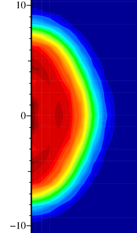
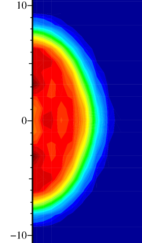
Figure 5: Density distribution for neutrons (left) and protons (right) in ${}^{158}_{\ 62}$Sm

Fig. 6 shows the corresponding pairing density for neutrons and protons; as discussed in ref.DN96 , this quantity describes the probability of correlated nucleon pair formation with opposite spin projection, and it determines the pair transfer formfactor. We can see that most correlated pair formation in ${}^{158}_{\ 62}$Sm takes place outside the central region of the nucleus.

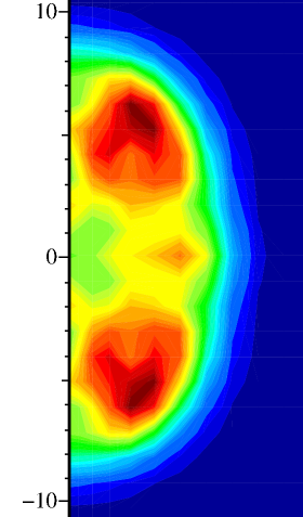
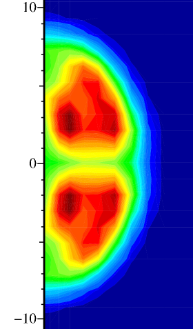
Figure 6: Pairing density distribution of neutrons (left) and protons (right) in ${}^{158}_{\ 62}$Sm

V Conclusions

In this paper, we have performed Skyrme-HFB calculations in coordinate space for several neutron-rich exotic nuclei. The coordinate space method has the advantage that well-bound, weakly bound and (discretized) continuum states can be represented with the same numerical accuracy. The novel feature of our lattice HFB code is that it takes into account high-energy continuum states with an equivalent single-particle energy of 60 MeV or more. This feature is crucial when one studies nuclei near the neutron dripline TOU03 .

We have calculated the ground state properties of the sulfur isotope chain ($Z=16$), starting at the line of stability ($N/Z=1$) up to the two-neutron dripline with a neutron-to-proton ratio of $N/Z\approx 2.2$. In particular, we have calculated two-neutron separation energies, quadrupole moments and rms radii for protons and neutrons. In comparing our HFB calculations with other theoretical methods (RMF with BCS pairing and HF+Lipkin/Nogami) we find similar results near stability but dramatic differences near the 2n-dripline (see Figures 1 - 4). For example, our HFB calculations predict ${}^{50}S$ to be the last isotope that is stable against the emission of two neutrons whereas the RMF approach predicts $S_{2n}(Z,N)>0$ at least up to ${}^{56}S$. For ${}^{48}S$, the last even-even isotope for which experimental binding energies are available (Fig. 1), the experimental value for the two-neutron separation energy is $3.64$ MeV, as compared to our HFB calculation result of $3.49$ MeV and the RMF result of $5.24$ MeV. Both our HFB calculations and the RMF calculations of ref.LR99 predict the existence of shape isomeric states in the neutron-rich sulfur isotopes. In Fig. 2 we compare calculated electric quadrupole moments. In most cases, the HFB and RMF calculations yield prolate quadrupole deformations. However, for the most neutron-rich sulfur isotopes, our HFB theory predicts a prolate ground state whereas RMF theory yields an oblate shape. Shape coexistence is found both in the HFB and RMF calculations, with fairly small energy difference between the ground state and the shape isomer. Specific results are given for ${}^{48}_{16}S_{32}$. A comparison between the root-mean-square radii of protons and neutrons clearly exhibits the development of a “neutron skin” in the neutron rich sulfur isotopes: for example, in ${}^{50}_{16}S_{34}$ our HFB calculations yield neutron and proton rms radii of $r_{n}=3.935$ fm and $r_{p}=3.364$ fm, respectively.

In connection with recent experiments at Gammasphere, we have carried out HFB calculations of medium/heavy mass nuclei with $N/Z\approx 1.6$. In particular, we have examined the isotopes ${}^{102,104}Zr$, ${}^{152}Ce$, ${}^{156}Nd$, and ${}^{158,160}Sm$. The theoretical quadrupole charge deformations for zirconium and cerium are in very good agreement with the new data. Also, our calculated proton rms radius for ${}^{102}Zr$ agrees with recent laser spectroscopic measurements. Table 1 gives a summary of these results and presents predictions for two neutron-rich isotopes, ${}^{156}Nd$ and ${}^{160}Sm$, for which experimental data are expected to become available in the near future.

- (1) “Opportunities in Nuclear Science, A Long-Range Plan for the Next Decade”, DOE/NSF Nuclear Science Advisory Committee, April 2002; published by US Dept. of Energy.
- (2) A.T. Kruppa, M. Bender, W. Nazarewicz, P.-G. Reinhard, T. Vertse, and S. Cwiok, Phys. Rev. C 61, 034313 (2000).
- (3) P. Navratil, J.P. Vary, and B.R. Barrett, Phys. Rev. C 62, 054311 (2000).
- (4) P. Navratil and W.E. Ormand, Phys. Rev. Lett. 88, 152502 (2002).
- (5) S.E. Koonin, D.J. Dean and K. Langanke, Phys. Rep. 278, 1 (1997).
- (6) T. Papenbrock and D.J. Dean, Phys. Rev. C 67, 051303(R) (2003).
- (7) T.R. Werner, J.A. Sheikh, W. Nazarewicz, M.R. Strayer, A.S. Umar, and M. Misu, Phys. Lett. B 333, 303 (1994).
- (8) J. Dobaczewski, W. Nazarewicz, T.R. Werner, J.F. Berger, C.R. Chinn and J. Dechargé, Phys. Rev. C 53, 2809 (1996).
- (9) J. Terasaki, P.-H. Heenen, H. Flocard and P. Bonche, Nucl. Phys. A600, 371 (1996).
- (10) E. Chabanat, P. Bonche, P. Haensel, J. Meyer and R. Schaeffer, Nucl. Phys. A635, 231 (1998); Nucl. Phys. A643, 441 (1998).
- (11) P.-G. Reinhard, D.J. Dean, W. Nazarewicz, J. Dobaczewski, J. A. Maruhn and M.R. Strayer, Phys. Rev. C 60, 014316 (1999).
- (12) M.V. Stoitsov, J. Dobaczewski, P. Ring and S. Pittel, Phys. Rev. C 61, 034311 (2000).
- (13) M. Yamagami, K. Matsuyanagi, and M. Matsuo, Nucl. Phys. A693, 579 (2001).
- (14) E. Terán, V.E. Oberacker, and A.S. Umar, Phys. Rev. C 67, 064314 (2003).
- (15) P. Ring, Prog. Part. Nucl. Phys. 37, 193 (1996).
- (16) G.A. Lalazissis, S. Raman, and P. Ring, Atomic Data and Nuclear Data Tables 71, 1 (1999).
- (17) M. Matsuo, Nucl. Phys. A696, 371 (2001).
- (18) M. Bender, J. Dobaczewski, J. Engel, and W. Nazarewicz, Phys. Rev. C 65, 054322 (2002).
- (19) I. Stetcu and C.W. Johnson, Phys. Rev. C 67, 044315 (2003).
- (20) J. Terasaki, Oak Ridge National Laboratory, private communication.
- (21) J.L. Egido, L.M. Robledo, and Y. Sun, Nucl. Phys. A560, 253 (1993).
- (22) A.S. Umar, J. Wu, M.R. Strayer and C. Bottcher, J. Comp. Phys. 93, 426 (1991).
- (23) J.C. Wells, V.E. Oberacker, M.R. Strayer and A.S. Umar, Int. J. Mod. Phys. C6, 143 (1995).
- (24) D.R. Kegley, V.E. Oberacker, M.R. Strayer, A.S. Umar and J.C. Wells, J. Comp. Phys. 128, 197 (1996).
- (25) V.E. Oberacker and A.S. Umar, in “Perspectives in Nuclear Physics”, ed. J.H. Hamilton, H.K. Carter, and R.B. Piercey, World Scientific (1999), pp. 255-266.
- (26) E. Terán, V.E. Oberacker, and A.S. Umar, Heavy-Ion Physics, Vol. 16/1-4, 437 (2002).
- (27) A.S. Umar, V.E. Oberacker, and E. Terán, Proc. Third Int. Conf. on “Fission and Properties of Neutron-Rich Nuclei”, Sanibel Island, Florida, November 3-9, 2002; World Scientific (2003), in print.
- (28) Half lives of isomeric states from SF of 252Cf and large deformations in 104Zr and 158Sm, J.K. Hwang, A.V. Ramayya, J.H. Hamilton, D. Fong, C.J. Beyer, P.M. Gore, E.F. Jones, E. Terán, V.E. Oberacker, A.S. Umar, Y.X. Luo, J.O. Rasmussen, S.J. Zhu, S.C. Wu, I.Y. Lee, P. Fallon, M.A. Stoyer, S. J. Asztalos, T.N. Ginter, J.D. Cole, G.M. Ter-Akopian, and R. Donangelo, subm. to Phys. Rev. C (July 2003).
- (29) O. Sorlin et al., Phys. Rev. C 47, 2941 (1993).
- (30) G. Audi and A.H. Wapstra, Nucl. Phys. A595, 409 (1995); and “Table of Nuclides”, Brookhaven Nat. Lab., http://www2.bnl.gov/ton/index.html.
- (31) N. Stone, “Table of Nuclear Moments (2001 Preprint)”, Oxford University, United Kingdom, http://www.nndc.bnl.gov/nndc/stone_moments/.
- (32) P. Campbell et al., Phys. Rev. Lett. 89, 082501 (2002).
- (33) H. Scheit et al., Phys. Rev. Lett. 77, 3967 (1996).
- (34) T. Glasmacher et al., Phys. Lett. B 395, 163 (1997).