Universal Transition Curve
in Pseudo-Rapidity Distribution

Abstract

We show that an unambiguous way of determining the universal limiting fragmentation region is to consider the derivative ($d^{2}n/d\eta^{2}$) of the pseudo-rapidity distribution per participant pair. In addition, we find that the transition region between the fragmentation and the central plateau regions exhibits a second kind of universal behavior that is only apparent in $d^{2}n/d\eta^{2}$. The $\sqrt{s}$ dependence of the height of the central plateau $(dn/d\eta)_{\eta=0}$ and the total charged particle multiplicity $n_{\rm total}$ critically depend on the behavior of this universal transition curve. Analyzing available RHIC data, we show that $(dn/d\eta)_{\eta=0}$ can be bounded by $\ln^{2}s$ and $n_{\rm total}$ can be bounded by $\ln^{3}s$. We also show that the deuteron-gold data from RHIC has the exactly same features as the gold-gold data indicating that these universal behaviors are a feature of the initial state parton-nucleus interactions and not a consequence of final state interactions. Predictions for LHC energy are also given.

I Introduction

Recently, PHOBOS and BRAHMS collaborations at RHIC published a set of intriguing data. Among them are the striking feature of the limiting fragmentation Back:2002wb ; Bearden:2001qq . It is reported by PHOBOS that the shifted (by the beam rapidity ${y_{\rm max}}$) pseudo-rapidity distribution per participant pair ${dn/d\eta}\equiv(dN_{\rm ch}/d\eta)/(N_{\rm part}/2)$ is independent of colliding energy up to 85-90 % of the plateau height Back:2002wb .

If taken at face value, this would imply that the height of the plateau and its $\sqrt{s}$ dependence would be almost fully determined by the limiting fragmentation curve and the location of the beginning of the plateau. Also, since the total multiplicity is simply the area under $dn/d\eta$, its $\sqrt{s}$ dependence would be largely determined by the limiting fragmentation curve as well.

It is not easy to determine the validity of above statements when only the rapidity distributions ($dn/d\eta$) are compared. In this paper we argue that comparing the slopes ($d^{2}n/d\eta^{2}$) is a much better way to determine various regions of the rapidity distribution.

A surprising feature is the existence of another ‘universal’ behavior, which is only apparent in the slopes. It turns out that $d^{2}n/d\eta^{2}$ in the transition region between the limiting fragmentation and the central plateau also follows a universal curve. This is not an extension of the limiting fragmentation curve. To our knowledge, this is the first time the existence of this second universal curve is demonstrated. These two universal curves basically determine the $dn/d\eta$. The energy dependence shows up through the position of the beginning of the central plateau.

The hypothesis of limiting fragmentation has a long history. For hadron-hadron collisions, this hypothesis was first put forward by Benecket et.al.Benecke:sh and also by FeynmanFeynman:ej and HagedornHagedorn:gh . This idea was further developed in Refs.Chou:bj – Hoang:1995mk .

Feynman hypothesized that as $\sqrt{s}\to\infty$, the multiplicity spectrum

$$\lim_{\sqrt{s}\to\infty}E_{p}\,{dn_{hh}\over d^{3}p}=\lim_{\sqrt{s}\to\infty}{dn_{hh}\over dy\,d^{2}p_{T}}=f(x_{L},p_{T})$$ (1)

becomes independent of $\sqrt{s}$. Here $y=(1/2)\ln((E_{p}+p_{L})/(E_{p}-p_{L}))$ is the rapidity and $x_{L}=2p_{L}/\sqrt{s}$ is the longitudinal momentum fraction. If the mass of the particles is light compared to the average $p_{T}$, this expression also equals $dn_{hh}/d\eta\,d^{2}p_{T}$ where $\eta=(1/2)\ln((p+p_{L})/(p-p_{L}))$ is the pseudo-rapidity. The universal function $f(x_{L},p_{T})$ then totally determines the height of the $dn_{hh}/d\eta$ and the total multiplicity at high energies.

Note that since $f(x_{L},p_{T})$ itself is independent of $\sqrt{s}$, the height of the plateau $\left(dn_{hh}/dy\right)_{\eta=0}$ must also be independent of $\sqrt{s}$. This also implies that the total multiplicity must behave like ${y_{\rm max}}\sim\ln s$ where

$${y_{\rm max}}=\cosh^{-1}(\sqrt{s}/2m_{N})\approx\ln(\sqrt{s}/m_{N})$$ (2)

is the beam rapidity and $m_{N}$ is the nucleon mass. However, up to $\sqrt{s}=1800\,\hbox{\,GeV}$ the experimental data does not show that $(dn/d\eta)_{\eta=0}$ is saturated. Also proton-proton and proton-anti-proton data show that the height of the plateau grows like $\ln^{2}s$ (See compilation by PHOBOS in Refs.Back:2003xk ; Back:2001ae .). The the total multiplicity then must grow like $\ln^{3}s$. This is not what one would expect from Eq.(1).

The source of this discrepancy is the fact the strict Feynman-Yang scaling is not perfect nor is it supposed to be. The central region (or small $x_{L}$) is modified by radiation of soft partons and and the multiple rescatterings of produced particles. QCD radiative corrections should also give rise to the additional scale dependence in $f(x_{L},p_{T})$Jalilian-Marian:2002wq .

However, within the dynamic range where Feynman-Yang scaling approximately holds, what should still work is the universality of $dn/d\eta$ near $\eta={y_{\rm max}}$, or equivalently at large $x_{L}$. We should still have

$$\left.{dn_{hh}\over d\eta}\right|_{\eta={y_{\rm max}}+\eta^{\prime}} \approx \int d^{2}p_{T}\,f((p_{T}/m_{N})\,e^{\eta^{\prime}},p_{T})\equiv f_{U}(\eta^{\prime})$$ (3)

where the universal function $f_{U}(\eta^{\prime})$ is independent of $\sqrt{s}$ (modulo the separating scale dependence). So far this is what the experimental data seem to show in both hadron-hadron collisions and the heavy-ion collisions.

Physically, the existence of the limiting fragmentation is a consequence of having a universal large $x$ distributions in high energy hadrons combined with the short interaction range in the rapidity spaceIancu:2002vu . Therefore, learning about the limiting fragmentation is equivalent to learning about the universal large $x$ distribution.

In the popular Venugopalan-McLerran model of gluon dynamics, these large $x$ partons then act as the color source that generates the small $x$ partons. Therefore establishing the validity and also the form of the limiting fragmentation in heavy ion collisions can provide an important input for the bulk dynamics of the soft degrees of freedom.

As far as we can determine, the second universal curve in the transition region has never been studied before. In the following sections, we will argue that the appearance of the universal transition curve may be anticipated. However, further study is needed to uncover the true cause for this universality.

In this context, it is quite interesting that the deuteron-gold (d+Au) result contains the same fragmentation and transition region curve as the gold-gold (Au+Au) result. This is discussed in more detail in section II.2.

The rest of this paper is organized as follows. In section II, we analyze available RHIC data. A simple parametrization of $d^{2}n/d\eta^{2}$ is presented and its consequences explicitly calculated. The results from several theoretical models including HIJINGWang:1996yf , UrQMDBass:1998ca ; Bleicher:1999xi and a saturation modelKharzeev:2000ph ; Kharzeev:2001gp are compared against the universal curves. Using the two parametrizations of $dn/d\eta$ from previous sections, we make a prediction for LHC in section III. Discussions and Conclusions are given in section IV. Appendix A contains details of a calculation not shown in the main text. In Appendix B, we discuss the validity (or the lack of) the Wood-Saxon form of $dn/d\eta$ sometimes used to describe the data.

II Experimental Limiting Fragmentation and Transition Curves

II.1 Analysis of RHIC Au+Au

Figure 1: $d^{2}n/d{\eta^{\prime}}^{2}$ numerically calculated from the PHOBOS most central collision dataBack:2002wb . The triangles are for $\sqrt{s}=200\,\hbox{\,GeV}$, the squares are for $\sqrt{s}=130\,\hbox{\,GeV}$ and the circles are for $\sqrt{s}=19.6\,\hbox{\,GeV}$. Also shown are two choices of limiting fragmentation functions as explained in the text. The two arrows mark the starting point of the plateau (${\eta_{p}}-{y_{\rm max}}$) and the starting point of the fragmentation region (${\eta_{f}}-{y_{\rm max}}$) for $\sqrt{s}=200\,\hbox{\,GeV}$ curve.

Figure 2: $d^{2}n/d{\eta^{\prime\prime}}^{2}$ numerically calculated from the PHOBOS most central data Back:2002wb . Here $\eta^{\prime\prime}=\eta-{\eta_{p}}$ where ${\eta_{p}}$ is the location of the hump in $dn/d\eta$. The solid line is $g_{U}(\eta^{\prime\prime})=-0.65\,\eta^{\prime\prime}$.

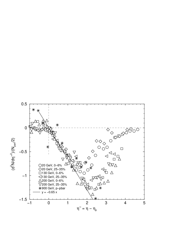
Figure 3: $d^{2}n/d{\eta^{\prime}}^{2}$ numerically calculated from the PHOBOS most central data and semi-central data Back:2002wb . Here $\eta^{\prime\prime}=\eta-{\eta_{p}}$ where ${\eta_{p}}$ is the location of the hump in $dn/d\eta$. The solid line is $g_{U}(\eta^{\prime\prime})=-0.65\,\eta^{\prime\prime}$.

If the universal behavior indeed extends up to 90 % of the plateau heightBack:2002wb , the height as well as the total multiplicity would be largely determined by the limiting function $f_{U}(\eta^{\prime})$ where $\eta^{\prime}\equiv\eta-{y_{\rm max}}$. In reality, the fragmentation region extend up to 50 % of the plateau height at RHIC energy. This fact is hard to see when comparing $dn/d\eta$’s but becomes apparent when comparing $d^{2}n/d\eta^{2}$’s. In Fig. 1, we plot $d^{2}n/d\eta^{2}$ for the most central collisions for $\sqrt{s}=200\,\hbox{\,GeV}$, $\sqrt{s}=130\,\hbox{\,GeV}$ and $\sqrt{s}=19.6\,\hbox{\,GeV}$ numerically calculated from the PHOBOS data. One can see that there are three distinct regions (we will ignore the hump). The limiting fragmentation region lies to the right of the minimum of $d^{2}n/d\eta^{2}$ ($\eta>{\eta_{f}}$) in which all data points merge together. To its left comes the transition region between the fragmentation and the plateau $({\eta_{p}}<\eta<{\eta_{f}})$. The zero of $d^{2}n/d\eta^{2}$ is where the plateau begins ($\eta={\eta_{p}}$). This is also the location of the hump in $dn/d\eta$.

It is clear from this figure that the true limiting fragmentation region starts from about half way between the plateau and ${y_{\rm max}}$. The area of the triangular shape is the height of the plateau. Therefore at these energies the limiting fragmentation region extends up to about 50 % of the maximum height. Apparent matching of data points below ${\eta_{f}}$ seen in $dn/d\eta^{\prime}$ is due to the slow change in the slope but it is not a true universal behavior.

What is even more interesting is that the transition region also exhibits a universal behavior. This is easily seen if one matches the zeros of $d^{2}n/d\eta^{2}$ curves (locations of the hump in $dn/d\eta$) as shown in Fig. 2. One can see that all data points again merge together. We will denote this ‘universal curve’ as

$$g_{U}(\eta^{\prime\prime})\equiv\left.{d^{2}n\over d\eta^{2}}\right|_{\eta={\eta_{p}}+\eta^{\prime\prime}}\ \ \ \ \ \ ({\eta_{p}}<\eta<{\eta_{f}})$$ (4)

In Fig. 3, we also show the semi-central data from PHOBOS together with the central collision data. The quality of the data is not as good as the central collision data, but the universal behavior is still evident. We do not plot very peripheral data in Fig. 3 since the participant scaling seems not to have been well established for them Back:2002wb . Instead, in Fig. 4, we plot the result of $p\bar{p}$ collisions at various high energies as measured at CERN together with a UrQMD calculation from Ref. Bleicher:1999pu and HIJING results. The quality of data for these measurements are not as clean as RHIC data from PHOBOS. However, there is a strong indication that there is a common transition curve. There is also an indication that the slope in $p\bar{p}$ $(-0.4)$ is different from the heavy ion result $(-0.65)$. As argued in Section II.2, this is most likely due to the nuclear modification which is also supported by the HIJING and UrQMD results shown in Fig. 4. From now on, we will focus our attention on the central heavy ion collisions.

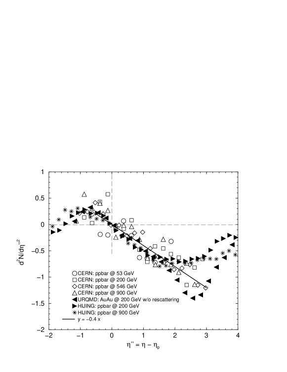
Figure 4: $d^{2}n/d{\eta^{\prime}}^{2}$ numerically calculated from CERN data as compiled by Particle Data GroupHagiwara:fs . Here $\eta^{\prime\prime}=\eta-{\eta_{p}}$ where ${\eta_{p}}$ is the location of the hump in $dn/d\eta$. The solid line is $g_{U}(\eta^{\prime\prime})=-0.40\,\eta^{\prime\prime}$.

The shape of $dn/d\eta$ is determined by the functional forms of $f^{\prime}_{U}(\eta^{\prime})=df_{U}/d\eta^{\prime}$ and $g_{U}(\eta^{\prime\prime})$ and the condition that these two curves meet at the transition point $\eta={\eta_{f}}$:

$$g_{U}({\eta_{f}}-{\eta_{p}})=f_{U}^{\prime}(-{y_{\rm max}}+{\eta_{f}})$$ (5)

This is the condition that connects the behavior of the fragmentation region to the plateau region. Once the value of ${\eta_{p}}$ is determined by the zero of $d^{2}n/d\eta^{2}$, the pseudo-rapidity distribution $dn/d\eta$ is fully determined by $f_{U}$, $g_{U}$ and the condition (5).

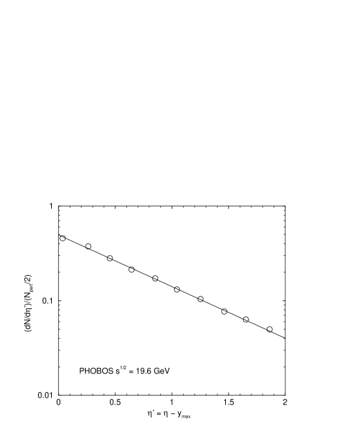
Figure 5: The tail part of the PHOBOS data on $dn/d\eta^{\prime}$ for the central 6 % of Au+Au collisions at $\sqrt{s}=19.6$ GeV. The straight line is $(dn/d\eta^{\prime})=0.492\,e^{-1.253\,\eta^{\prime}}$.

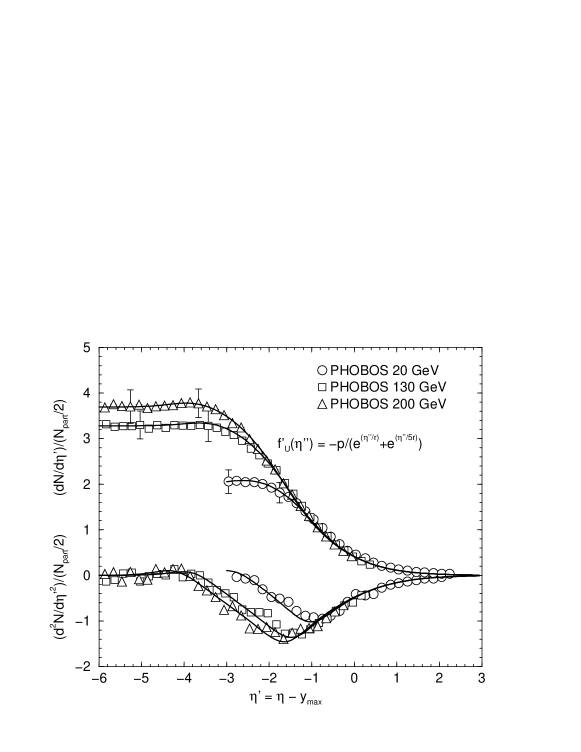
Figure 6: Pseudo-rapidity distribution for 6 % most central Au-Au collisions at $\sqrt{s}=200\,\hbox{\,GeV}$. Data are from Ref. Back:2002wb . Lower curves are $d^{2}n/d\eta^{2}$ calculated numerically from $dn/d\eta$ data. The solid lines are our fits. Here we used $\tilde{\theta}_{\rho}(x-x_{0})=1/(1+e^{-(x-x_{0})/\rho})$ with $\rho=0.25$ and the parameters are set to $p=0.95$, $1/r=0.308$, $q=r/5$, $\delta=0.3$ and $K=0.65$. The value of $p$ is different from 1.08 quoted in the text because a finite value of $\rho$ compensates it a little. Here ${\eta_{p}}$ is not free but fixed by the position of the hump. They are at $\eta^{\prime}=-3.96$, $\eta^{\prime}=-3.65$ and $\eta^{\prime}=-2.6$ for $\sqrt{s}=200,130,19.6\,\hbox{\,GeV}$ respectively.

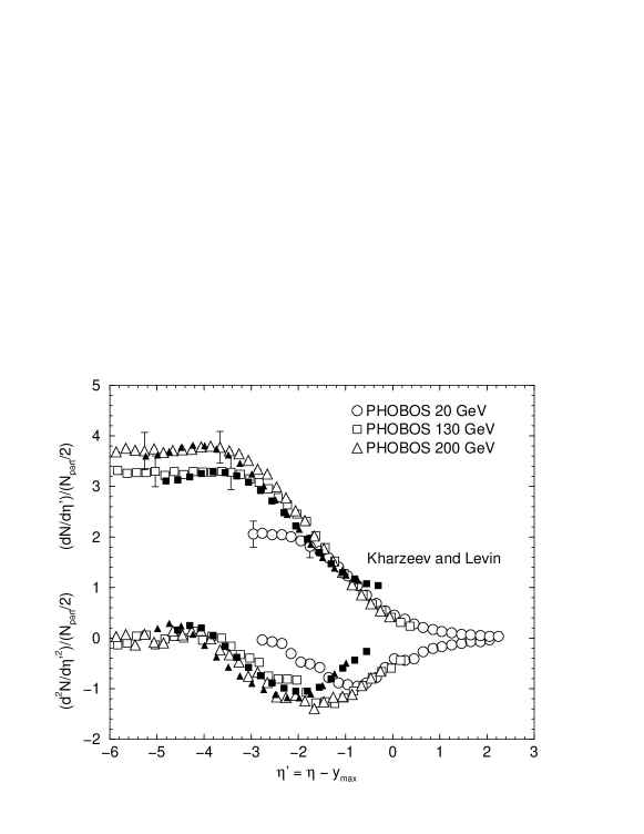
Figure 7: $dn/d\eta$ and $d^{2}n/d\eta^{2}$ calculated using Kharzeev and Levin’s resultKharzeev:2001gp . Open symbols are PHOBOS results and full symbols are the calculations.

Figure 8: $d^{2}n/d\eta^{2}$ calculated using Kharzeev and Levin’s resultKharzeev:2001gp up to the LHC energy.

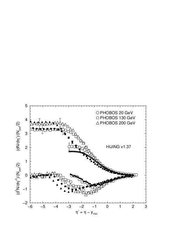
Figure 9: $dn/d\eta^{\prime}$ and $d^{2}n/d{\eta^{\prime}}^{2}$ from the central PHOBOS data compared with HIJING v1.37 (filled symbols) calculations with $dE/dx=-2$ GeV/fm ToporPop:2002gf .

Figure 10: $d^{2}n/d{\eta^{\prime}}^{2}$ numerically calculated from the central PHOBOS data compared with HIJING v1.37 calculations.

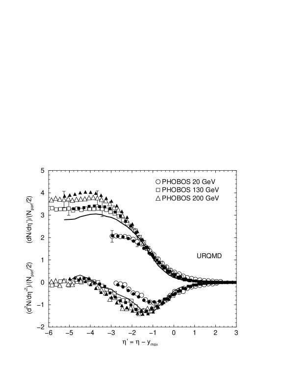
Figure 11: $d^{2}n/d{\eta^{\prime}}^{2}$ numerically calculated from the central PHOBOS data compared with UrQMD calculations (filled symbols). The solid line is UrQMD result for $\sqrt{s}=200\,\hbox{\,GeV}$ without rescatterings.

Figure 12: The derivative $(d^{2}N/d\eta^{2})/(N_{\rm part}/2)$ with respect to $\eta$. Data are taken from the PHOBOS websitephobosweb .

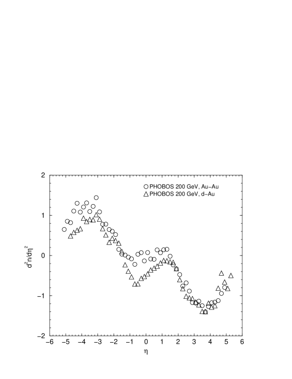
Figure 13: The same as Fig.12 but d+Au data is vertically scaled by a factor of 1.3 and shifted to the right by 0.4 unit of pseudorapidity (2 experimental bins).

Figure 14: The same as Fig.13 but for $dN/d\eta$.

Figure 15: The same as Fig.12 but d+Au data is vertically scaled by a factor of 1.9 and shifted to the right by 0.2 unit of pseudorapidity (1 experimental bin).

Figure 16: The same as Fig.15 but for $dN/d\eta$. d+Au result is shifted vertically down by 3.6.

Figure 17: Predictions for central collisions at LHC. Also shown are parametrized RHIC 200 result. We set $\sqrt{s}=5.5\,\hbox{TeV}$ and Pb+Pb for LHC.

A question then arises: What are the functional forms of the limiting fragmentation curve $f_{U}$ and the transition curve $g_{U}$? For the transition curve $g_{U}$, the current RHIC data shown in Fig. 2 suggest that it is a linear function of $\eta$ with a $\sqrt{s}$ independent slope. In this paper, we take this to be true and write

$$g_{U}(\eta^{\prime\prime})=-K\eta^{\prime\prime}$$ (6)

where $\eta^{\prime\prime}=\eta-{\eta_{p}}$. The value of $K$ we use is set to $0.65$ which is the slope of the straight line shown in Fig. (2).

As for the limiting fragmentation function, there is little doubt that $f_{U}$ is exponential for $\eta>{y_{\rm max}}$ as can be clearly seen in Fig. 5. But what about below ${y_{\rm max}}$? A current theoretical analysisJalilian-Marian:2002wq relates $f_{U}$ to the gluon distribution function at large $x$. At moderate $Q^{2}$, the gluon distribution function has the form

$$xG(x,Q^{2})\sim x^{-\lambda}\,(1-x)^{n}$$ (7)

With $x=e^{-2-{y_{\rm max}}+\eta}=e^{-2+\eta^{\prime}}$Jalilian-Marian:2002wq , this means that the limiting fragmentation function should behave like

$$f_{U}(\eta^{\prime})\sim e^{-\lambda\eta^{\prime}}(1-e^{-2+\eta^{\prime}})^{n}$$ (8)

Here $-2$ in the exponent is due to the mass difference between a proton and a pion. The behavior of the expression (8) is different from the exponential behavior shown in Fig. 5 in the $\eta^{\prime}>0$ $(\eta>{y_{\rm max}})$ region. However in the $\eta^{\prime}<0$ $(\eta<{y_{\rm max}})$ region,

$$f_{U}(\eta^{\prime})\sim e^{-\lambda\eta^{\prime}}$$ (9)

gives a reasonable description with $\lambda\sim 0.25$Jalilian-Marian:2002wq .

Combined, the above analysis indicate that the behavior of $dn/d\eta$ changes from one exponential form to another exponential form when $\eta$ crosses ${y_{\rm max}}$ (or $\eta^{\prime}$ crosses $0$). We may represent such behavior with

$$f^{\prime}_{U}(\eta^{\prime})\equiv{df_{U}\over d\eta^{\prime}}=-{p\over e^{\eta^{\prime}/r}+e^{\eta^{\prime}/q}}$$ (10)

In Fig. 1, the solid curve corresponds to this form fitted to $\eta^{\prime}>-1$ portion of the combined data set. The dashed curve corresponds to the extension of the exponential from $\eta^{\prime}>0$ region.

If the data points shown in Fig. 1 follow the true universal curve, then we have no choice but to conclude that $f_{U}$ changes its behavior once $\eta={y_{\rm max}}$ is crossed. On the other hand, we may also consider that RHIC energy is not high enough for the true universal curve to manifest and what we see in the current data is an accident. One such example is presented in Appendix B. For reasons explained in the Appendix, this accident is unlikely. However, only further experiments can give a definite verdict.

Using Eq. (6) for $g_{U}$, we write for $\eta>0$

$${d^{2}n\over d\eta^{\prime 2}}=-\left({p\over e^{\eta^{\prime}/r}+e^{\eta^{\prime}/q}}\right)\,\tilde{\theta}_{\rho}(\eta^{\prime}+{\chi_{f}})-K(\eta^{\prime}+{\chi_{p}})\,\tilde{\theta}_{\rho}(-{\chi_{f}}-\eta^{\prime})\,\tilde{\theta}_{\rho}(\eta^{\prime}+{\chi_{p}}-\delta)$$ (11)

where $\eta^{\prime}=\eta-{y_{\rm max}}$ and $\tilde{\theta}_{\rho}(x)$ is the smeared $\theta$ function with $\lim_{\rho\to 0}\tilde{\theta}_{\rho}(x)=\theta(x)$. The minimum of $d^{2}n/d\eta^{\prime 2}$ is located at $\eta^{\prime}=-{\chi_{f}}={\eta_{f}}-{y_{\rm max}}$ and the hump of $dn/d\eta^{\prime}$ is located at $\eta^{\prime}=-{\chi_{p}}={\eta_{p}}-{y_{\rm max}}$. The parameters $\delta$ and $\rho$ control the height and the width of the hump. The parameter $K=0.65$ is the slope of the transition region. By fitting the combined $\eta^{\prime}>-1$ data, we get $p=1.08$, $1/r=0.308$ and $1/q=1.566\approx 5/r$. We mention here that this $1/r$ value is fairly close to the value of a similar coefficient obtained from saturation model studiesJalilian-Marian:2002wq ; Kharzeev:2000ph ; Kharzeev:2001gp ; Kharzeev:2002pc ; Dumitru:2002wd ; Kovchegov:1999ep . The shape of $dn/d\eta$ obtained from Eq.(11) as well as $d^{2}n/d\eta^{2}$ itself is shown in Fig. 6. In the figure, $p=0.95$ is used because having finite $\rho$ changes the slope a little.

The transition between the fragmentation region and the transition region happens at $\eta^{\prime}=-{\chi_{f}}$ where the two lines meet. This yields the following condition

$$K({\chi_{p}}-{\chi_{f}})={p\over e^{-{\chi_{f}}/r}+e^{-{\chi_{f}}/q}}\approx p\,e^{{\chi_{f}}/r}$$ (12)

where the approximation works for large ${\chi_{f}}/r$. This is the condition which relates the limiting fragmentation to the plateau and ultimately determines the size of the fragmentation region. For large ${\chi_{f}}/r$, the solution is given by

$${\chi_{f}}\approx{\chi_{p}}-r\,W(e^{{\chi_{p}}/r}p/Kr)$$ (13)

where the Lambert function solves $w=W(w)\exp(W(w))$. With the values of the parameters from above, the approximation (13) is good within 1 % for RHIC and LHC but not for SPS. For future reference, we note that for large $w$, $W(w)\approx\ln w-\ln\ln w$. Hence

$${\chi_{f}}\sim\ln{\chi_{p}}\ll{\chi_{p}}$$ (14)

Integrating Eq.(11) from $\infty$ to $\eta^{\prime}$ gives the rapidity distribution $dn/d\eta^{\prime}$. Numerical integration yields excellent description of the existing data as shown in Fig. 6. Unfortunately, the form of $f_{U}^{\prime}(\eta^{\prime})$ in Eq.(10) does not allow analytic integration in general. However, note that $1/q\approx 5/r$. If $1/q=5/r$, the necessary integration can be carried out in the sharp $\theta$-function limit ($\tilde{\theta}_{\rho}\to\theta$). The resulting form is analytic but not very illuminating. Details can be found in Appendix A.

Now consider the height of the plateau, $(dn/d\eta)_{0}$. Note that the fragmentation region $d^{2}n/d\eta^{2}$ behaves exponentially while the transition region $d^{2}n/d\eta^{2}$ behaves linearly in $\eta$. Therefore in the large ${y_{\rm max}}$ limit, the contribution from the transition region dominates in $(dn/d\eta)_{0}$. Physically, this is what one would expect. At high enough energies, the dynamics of the central plateau region and the dynamics of the limiting fragmentation region should decouple and the height of the central plateau should not depend much on the exact form of $f_{U}$. The height of the plateau in the large ${y_{\rm max}}$ limit is then given by

$$\left(dn\over d\eta\right)_{0}\approx{K\over 2}\left({\chi_{f}}-{\chi_{p}}\right)^{2}+O({y_{\rm max}})$$ (15)

This implies

$$\left(dn\over d\eta\right)_{0}<{K\over 2}\ln^{2}(\sqrt{s}/m_{N})$$ (16)

since ${\eta_{p}}<{\eta_{f}}<{y_{\rm max}}$ and ${\chi_{f}}\sim\ln{\chi_{p}}$. Integrating once more, the total multiplicity can be obtained as

$$n_{\rm total} \approx {K\over 3}({\eta_{f}}-{\eta_{p}})^{2}(2{\eta_{f}}+{\eta_{p}})+O(y_{\rm max}^{2})$$ (17)

which implies

$$n_{\rm total}<{2K\over 3}\ln^{3}(\sqrt{s}/m_{N})$$ (18)

From Eqs.(15) and (17) we conclude that the central plateau cannot rise faster than $y_{\rm max}^{2}$ or $\ln^{2}s$ and the total multiplicity cannot rise faster than $y_{\rm max}^{3}$ or $\ln^{3}s$. The only possible way to get faster dependence is to have $\sqrt{s}$ dependent $K$, or faster rising $g_{U}$ (for instance an exponential). Judging from Fig. 4, this is not likely up to 900 GeV. Also there is an additional evidence from the CDF collaboration Abe:1989td that up to $\sqrt{s}=1.8\,\hbox{TeV}$, the central plateau in $p\bar{p}$ collisions rises only as fast as $\ln^{2}s$.

In many current models of heavy ion collisions, $n_{\rm total}$ grows faster than $\ln^{3}s$. For instance, Ref.Kharzeev:2001gp has $n_{\rm total}\sim s^{\lambda/2}$ and the $e^{+}e^{-}$ modelBack:2003xk has $n_{\rm total}\sim e^{c\sqrt{\ln s}}$ where $\lambda$ and $c$ are constants. Parametrization of $pp$, $pA$ and $AA$ data up to the SPS energy by Gazdzicki and HansenGazdzicki:ih gives $N_{\rm ch}\propto s^{1/4}$. At present energies, these are indistinguishable from polynomials in $\ln s$. However, as will be presented shortly, LHC will be able to tell whether the bound (18) indeed holds for high energy heavy ion collisions.

At this point, we can attempt a partial explanation of the appearance of the universal transition curve. Suppose that as the collision energy becomes larger the dynamics of plateau region largely decouples from the dynamics of the fragmentation region. This is certainly the case for the $f_{U}$ and $g_{U}$ given in this section as indicated by Eq.(14). Eq.(14) implies that in the large ${y_{\rm max}}$ limit, ${\eta_{f}}\gg{\eta_{p}}$ and

$${\eta_{f}}={y_{\rm max}}+O(\ln{y_{\rm max}})\,.$$ (19)

This is a consequence of having an exponential fragmentation curve and a polynomial transition curve. Note that the functional form of $g_{U}$ and $f_{U}$ enters only through the logarithmic correction.

At RHIC energies, the area under $f_{U}$ and $g_{U}$ looks like an isosceles triangle. This is because $\ln{y_{\rm max}}$ is still not that small compared to ${y_{\rm max}}$. However since an exponential rises fast, the area will look more and more like a right triangle as the energy grows and the area will become dominated by the transition part:

$$\left(dn\over d\eta\right)_{0} \approx \int^{{\eta_{p}}}_{{\eta_{f}}}d\eta\,g_{U}(\eta-{\eta_{p}})$$ (20)

$$= -\int^{{\eta_{f}}-{\eta_{p}}}_{0}d\eta^{\prime\prime}\,g_{U}(\eta^{\prime\prime})\approx-\int^{{y_{\rm max}}}_{0}d\eta^{\prime\prime}\,g_{U}(\eta^{\prime\prime})\,.$$

Therefore, to leading order in ${y_{\rm max}}$, $\left(dn/d\eta\right)_{0}$ is a function of ${y_{\rm max}}\approx\ln(\sqrt{s}/m_{N})$ and it is independent of the functional form of the fragmentation curve $f_{U}$. Denoting the functional dependence as $(dn/d\eta)_{0}=S({y_{\rm max}})$, the universality of $g_{U}$ follows if the following relationship holds

$$g_{U}(\eta^{\prime\prime})\approx-{dS(\eta^{\prime\prime})\over d\eta^{\prime\prime}}\,.$$ (21)

Once the dependence of $\left(dn/d\eta\right)_{0}$ on $\sqrt{s}$ is given, $g_{U}$ is totally determined and it is indeed universal up to logarithmic corrections. The relation (21) certainly holds for Eqs.(6) and (15) when ${y_{\rm max}}\gg 1$.

The hole in this argument is that the relationship (20) does not automatically imply Eq.(21). For instance, suppose $S({y_{\rm max}})=ay_{\rm max}^{2}$. In this case, any

$$g_{U}(\eta^{\prime})={a\,n\,y_{\rm max}^{2-n}}\,(\eta^{\prime\prime})^{n-1}$$ (22)

with $n>1$ satisfies Eq.(20). Unless $n=2$, however, $g_{U}(\eta^{\prime\prime})$ depends on ${y_{\rm max}}$ and hence it is not universal. Surprising fact is that the data seems to suggest $n$ is indeed 2 or at least very close to it.

The relationship (21) is remarkable. It relates an observable that is a function of colliding energy to an observable that is a function of the pseudo-rapidity at any fixed energy. Unfortunately, energies probed so far are too small for this to manifest. As seen in Figures 2-4, the transition region is not truly dominant yet. However, we should be able to test this relationship at LHC.

It is also instructive to compare some theory curves with RHIC data as shown in Figs. 7-11. As shown in Figs.7 the saturation model by Kharzeev and LevinKharzeev:2001gp gives a good description of the plateau and the transition region at RHIC energy although the fragmentation region is badly off. However, since the model is based on small $x$ picture, it is not supposed to be valid in the fragmentation region. From the expression of $dn/dy$ given in Ref.Kharzeev:2001gp , it is clear that the transition curve obtained by Kharzeev and Levin is exponential and this form of $dn/dy$ does not satisfy the relation (21). The reason Fig. 8 shows approximate universal behavior up to $\sqrt{s}=1000\,\hbox{\,GeV}$ is $\lambda$ is small. At LHC energy, the violation of the universality is clearly seen for this model.

HIJING results ToporPop:2002gf ; Wang:2000bf with shadowing and a parton energy loss of $dE/dx=-2$ GeV/fm and an energy dependent scale parameter $p_{0}$ as considered in Li:2001xa are shown in Fig.9. It is quite evident in the $d^{2}n/d\eta^{2}$ plot that the fragmentation region dominates in HIJING. Again to test the transition curve universality, one must go beyond the RHIC energy. Fig.10 shows $d^{2}n/d\eta^{2}$ up to the LHC energy. From the figure, it is quite clear that HIJING does not contain a universal transition curve. Furthermore, at higher energies, the central region develops a bump instead of a plateau. This feature is due to the abundance of the minijets. As can be seen in Fig. 17, by enhancing the parameter $p_{0}$ (equivalently, reducing the number of minijets) HIJING becomes closer to the other models. But the transition region universality is clearly not a feature in the HIJING model.

On the other hand, it is quite striking that the default UrQMD results get both $dn/d\eta$ and $d^{2}n/d\eta^{2}$ right at RHIC energies. It is also significant that without rescatterings, UrQMD does not describe the data well. Why UrQMD results in universal transition curve is not yet clear.

II.2 Analysis of RHIC d+Au

Recently the PHOBOS collaboration published the result of measuring the pseudorapidity distribution of produced particles in the deuteron-gold (d+Au) collisions at $\sqrt{s}=200\,\hbox{\,GeV}$Back:2003hx . At a first glance, it would seem that there is no common feature at all between the d+Au $dn/d\eta$ and Au+Au $dn/d\eta$, especially if one just looks at the participant-scaled results. However, when dealing with very asymmetric systems such as d+Au, one must be careful about the scaling behavior. As can be easily shown in a simple wounded nucleon model, the scaling of produced particles in the heavy ion side and the d side should be different. The number of wounded nucleons in the heavy ion side depends on the linear size of the heavy ion whereas the d side always have 1 or 2 wounded nucleons. Hence, the multiplicity in the heavy ion side should have an additional scale factor $\sim A^{1/3}$ compared to the d side.

To see whether there is a common feature between Au+Au and d+Au or not, again it is much better to look at the derivative $(d^{2}N/d\eta^{2})/(N_{\rm part}/2)$ as shown in in Fig.12. Judging from this figure, it is clear that there is a common feature. To bring it out more clearly, we vertically scale the d+Au result by a factor of 1.3 and shift it horizontally by 0.4 unit of rapidity (or 2 experimental bins). This results in Figs. 13 and 14 which leaves no room for doubt that the shape of $dN/d\eta$ for $\eta>1.5$ is common to both Au+Au and d+Au results. It is also interesting to see that different scaling (additional factor of 1.5 compared to Fig.13 and the rapidity shift of $0.2$ (or 1 experimental bin) instead of 0.4) brings the Au side of the spectrum together as shown in Fig.15. and Fig.16. Again, there is no room for doubt that there is a common curve. This implies that beside a constant component, the shape of $dn/d\eta$ for both Au+Au and d+Au is simply related by scaling even in the Au side.

III Prediction For LHC

Given the two forms of parametrization considered in the previous sections, it is possible to extrapolate and predict what should happen at LHC where $\sqrt{s}=5500\,\hbox{\,GeV}$ and ${y_{\rm max}}=8.68$. To do so, we need to parametrize the functional form of ${\eta_{p}}$ or ${\eta_{f}}$. The value of ${\eta_{p}}$ in the model from section II.1 is not a free parameter. The position of the hump clearly visible in $d^{2}n/d\eta^{2}$ as a zero is the value of ${\eta_{p}}$. From the PHOBOS data, one gets, ${y_{\rm max}}-{\eta_{p}}=3.96,3.65$ for $\sqrt{s}=200,130\,\hbox{\,GeV}$. For $\sqrt{s}=19.6\,\hbox{\,GeV}$ case, the data has ${y_{\rm max}}-{\eta_{p}}=2.75$. However, with our model, ${y_{\rm max}}-{\eta_{p}}=2.6$ describes the data better.

By fitting the above values of ${\eta_{p}}$ with ${y_{\rm max}}-{\eta_{p}}=\lambda y^{\nu}+\beta\ln y$ and ${y_{\rm max}}-{\eta_{p}}=\lambda y^{\nu}+C$, we get

$${y_{\rm max}}-{\eta_{p}}=\left\{\begin{array}[]{ll}0.60+0.73\,y_{\rm max}^{0.91}&\ \ (\hbox{Model I})\\ 0.33\ln{y_{\rm max}}+0.96\,y_{\rm max}^{0.75}&\ \ (\hbox{Model II})\end{array}\right.$$ (25)

These two parametrizations do not differ much up to ${y_{\rm max}}=10$. The LHC predictions from these two parametrizations are given in Table 1. The shape of $dn/d\eta$ is given in the Fig 17 together with the Kharzeev-Levin prediction and the HIJING predictions with two different minimum minijet energies. The results obtained for $p_{0}=3.5\,\hbox{\,GeV}$ suggested in reference Li:2001xa , is clearly very different from other models. Increasing the mini-jet scale parameter to a higher value $p_{0}=7.0\,\hbox{\,GeV}$ brings it to a better agreement with other models. Only data from LHC will allow us to draw a definite conclusion and to choose the right value for this parameter $p_{0}$.

One striking feature is that in both the Kharzeev-Levin model and the HIJING model with $p_{0}=3.5\,\hbox{\,GeV}$, the central plateau disappear. This is mainly due to the fact that these models do not contain rescatterings of the secondaries and hence cannot not undergo a Bjorken-like expansion.

	${y_{\rm max}}-{\eta_{p}}$	$(dn/d\eta)_{0}$	$n_{\rm total}$
Model I	5.8	6.9	87
Model II	5.6	6.5	83
K & L	–	10.7	110
HIJING w/ $p_{0}=3.5\,\hbox{\,GeV}$/c	–	21.4	160
HIJING w/ $p_{0}=7.0\,\hbox{\,GeV}$/c	–	11.6	100

Table 1: Predictions for LHC central collisions. We set $\sqrt{s}=5.5\,\hbox{TeV}$ and Pb+Pb for LHC.

.

IV Discussions and Conclusions

In this paper, we showed that there exists a second universal behavior in the rapidity distribution of produced particles. The data we have analyzed clearly indicate that $d^{2}n/d\eta^{2}$’s in the transition region taken at different energies follow a common curve. This is not easy to see when comparing $dn/d\eta$’s but clearly seen when comparing $d^{2}n/d\eta^{2}$’s.

We emphasize here that any model that purports to describe the rapidity distribution in the whole rapidity space must be able to reproduce not only the limiting fragmentation curve, but also the universal transition curve.

The existence of the two universal curves implies that the shape and the size of the rapidity distribution itself is mostly determined by (i) the limiting fragmentation curve $f_{U}$, (ii) the universal transition curve $g_{U}$ and (iii) the starting point of the plateau region ${\eta_{p}}$. Non-trivial physics resides in the $\sqrt{s}$ dependence of ${\eta_{p}}$ or equivalently the size the central plateau.

The physics behind the limiting fragmentation curve is well known to be the Feynman-Yang scaling which states that at high energy, large $x_{L}$ behavior of an inclusive cross-section is independent of $\sqrt{s}$. In this paper we argued that the physics behind the universal transition curve is in fact the decoupling between the dynamics of the plateau and the fragmentation region. We note that it is also intriguing that perhaps a connection to the gluon parton distribution can be made. In saturation models, $dn/d\eta$ is related to the gluon distribution functionKharzeev:2000ph ; Jalilian-Marian:2002wq ; Kharzeev:2001gp . In this case, the universal transition curve puts a severe restriction on the behavior of the gluon distribution at moderate $x$.

In this work, we found that the universal transition curve is linear in $\eta^{\prime\prime}=\eta-{\eta_{p}}$ based on $\sqrt{s}=20-200\,\hbox{\,GeV}$ RHIC data and UA5 $p\bar{p}$ data. A consequence of having a linear transition curve is that the plateau height $(dn/d\eta)_{0}$ cannot grow faster than $\ln^{2}s$ and the total charged multiplicity cannot grow faster than $\ln^{3}s$. This polynomial behavior in $\ln s$ is maintained if the transition curve is polynomial in $\eta^{\prime\prime}$. A power law growth $(dn/d\eta)_{0}\sim s^{\lambda}$ or an $e^{+}e^{-}$ type exponential growth is possible only if the transition curve is exponential. The available data does not show such exponential behavior. It does not, of course, rule out a change in the behavior at higher energies. As shown in the last section, these possibilities can be clearly distinguished at LHC.

What we have found in this study also impacts hydrodynamic studies. As can be seen in Eq.(25) the size of the plateau does not grow fast. Moreover as ${y_{\rm max}}\to\infty$, ${\eta_{p}}/{y_{\rm max}}\to 0$. Therefore, the relative region of validity for 2-D hydrodynamic calculation shrinks as the energy goes up and the need for 3-D hydrodynamic calculation becomes greater. Furthermore, the existence of the universal transition curve will tightly constrain the longitudinal evolution of the hydrodynamic system.

We have also analyzed the deuteron-gold result from RHIC and found that there is a single common curve that determines the shape of $dN/d\eta$ for both d+Au and Au+Au cases. A few conclusions can be drawn from our analysis. First of all, the different scaling factors for the deuteron side and the gold side indicate that the scaling of d+Au system is more complex than a simple participant scaling. This implies that using a simple participant scaling can potentially mislead the comparision between the d+Au result and Au+Au result. This is especially significant for the Au side where there appears to be a constant component on top of the two universal curves discussed in this paper. Again, these facts are much more transparent if one compares $d^{2}N/d\eta^{2}$.

Second, the existence of a function common to both Au+Au and d+Au indicates that the dynamics of the transition region and the fragmentation region in the Au+Au case cannot depend much on the final state interactions. It can only depend on initial state parton-nucleus dynamics. Especially, whether or not a hot and dense system is formed in Au+Au collisions does not influence the shape of $dN/d\eta$ beyond the plateau region.

The exact physical meaning of the rapidity shifts and the constant component in the d+Au data are under investigation.

Appendix A Integral over $df_{U}/d\eta^{\prime}$

To calculate $dn/d\eta$, we need

$$\int_{\infty}^{\eta^{\prime}}d\eta^{\prime\prime}\,{df_{U}\over d\eta^{\prime\prime}} = -p\int_{\infty}^{\eta^{\prime}}d\eta^{\prime\prime}\,{1\over e^{\eta^{\prime}/r}+e^{5\eta^{\prime}/r}}$$ (26)

Changing variable to $y=e^{\eta^{\prime\prime}/r}$ yields

$$-p\,r\int_{\infty}^{e^{\eta^{\prime}/r}}{dy\over y^{2}(1+y^{4})} = -p\,r\int_{\infty}^{e^{\eta^{\prime}/r}}dy\,\left({1\over y^{2}}-{y^{2}\over 1+y^{4}}\right)$$ (27)

These integrals can be found in integral tables, for instance Ref.integ:GR . We get

$$\int_{\infty}^{\eta^{\prime}}d\eta^{\prime\prime}\,{df_{U}\over d\eta^{\prime\prime}} = p\,r\,\Bigg{\{}e^{-\eta^{\prime}/r}+{p\over 2\sqrt{2}}\left(\tan^{-1}\left(1+\sqrt{2}e^{\eta^{\prime}/r}\right)-\tan^{-1}\left(1-\sqrt{2}e^{\eta^{\prime}/r}\right)-\pi\right)$$ (28)

$${}\qquad-{1\over 2}\log\left(1+\sqrt{2}e^{-\eta^{\prime}/r}+e^{-2\eta^{\prime}/r}\over 1-\sqrt{2}e^{-\eta^{\prime}/r}+e^{-2\eta^{\prime}/r}\right)\Bigg{\}}$$

Appendix B Universal Fragmentation Condition for Wood-Saxon

A popular choice of parametrization for $dn/d\eta$ is the Wood-Saxon function. Many models for hadron-hadron collisions developed in the 70’s Ranft:tf ; Bali:as ; Bali:ap ; Bali:rk ; Boggild:sh also had this type of $dn/d\eta$. As will be shortly shown, this Wood-Saxon form is not compatible with the transition region universality and hence it is unlikely that this is the right form of $dn/d\eta$. Nevertheless we feel that it is worth considering the Wood-Saxon form here because it gives an example of slowly changing (as opposed to universal) limiting fragmentation curve.

A reasonable description of the current data can be provided by the following combination of the Wood-Saxon (Fermi-Dirac) functions and a hyperbolic cosineEskola:2002qz

$${dn\over d\eta}={g\,\cosh(\eta/\zeta)\over[1+e^{-(\eta+{\eta_{f}})/\sigma}][1+e^{(\eta-{\eta_{f}})/\sigma}]}$$ (29)

where $g$, ${\eta_{f}}$, $\zeta$ and $\sigma$ are functions of ${y_{\rm max}}$. Here the parameter ${\eta_{f}}$ roughly corresponds to where the fragmentation region begins. The hyperbolic cosine is there to provide the dip in the middle. Since the dip is usually shallow, $\zeta\gg\sigma$.

Since we are not so much interested in the dip, we consider a simplified form

$${dn\over d\eta}={g\over 1+e^{(\eta-{\eta_{f}})/\sigma}}\ \ \ \ \ \hbox{for}\ \ \eta>0$$ (30)

Universal fragmentation behavior demands that for high enough energy

$$\left.{dn\over d\eta}\right|_{\eta={y_{\rm max}}+\eta^{\prime}}=f_{U}(\eta^{\prime})$$ (31)

where $f_{U}(\eta^{\prime})$ is indepdent of ${y_{\rm max}}$. If ${\eta_{f}}/\sigma\gg 1$, this just implies that $g=\kappa_{0}e^{({y_{\rm max}}-{\eta_{f}})/\sigma}$ so that it compensates the large exponential in the denominator. Near $\eta={y_{\rm max}}$ this yields $f_{U}(\eta^{\prime})=\kappa_{0}\,e^{-\eta^{\prime}/\sigma}$. However at SPS and RHIC energy, ${y_{\rm max}}$ is only about 3 to 5 and it can be easily shown that simply having $g=\kappa_{0}e^{({y_{\rm max}}-{\eta_{f}})/\sigma}$ with a constant $\sigma$ does not result in the universal limiting fragmentation. Instead, we must regard all parameters appearing in Eq.(30) as functions of ${y_{\rm max}}$ and look for a relationship among them by requiring

$${\partial\over\partial{y_{\rm max}}}{dn\over d\eta^{\prime}}\approx 0$$ (32)

near $\eta={y_{\rm max}}$ (or $\eta^{\prime}=\eta-{y_{\rm max}}=0)$.

The solution of Eq.(32) is obtained as follows. Set $\sigma=1/\tau$ and $\eta={y_{\rm max}}+\eta^{\prime}$ and ${\chi_{f}}={y_{\rm max}}-{\eta_{f}}$ and write

$$f\equiv{dn\over d\eta^{\prime}}={g\over 1+e^{(\eta^{\prime}+{\chi_{f}})\tau}}$$ (33)

Taking the derivative with respect to $y={y_{\rm max}}$ yields

$${\partial f\over\partial y} = {(dg/dy)(1+e^{(\eta^{\prime}+{\chi_{f}})\tau})-g\left[\eta^{\prime}(d\tau/dy)+d({\chi_{f}}\tau)/dy\right]e^{(\eta^{\prime}+{\chi_{f}})\tau}\over(1+e^{(\eta^{\prime}+{\chi_{f}})\tau})^{2}}$$ (34)

If this is to be independent of $\eta^{\prime}$ for small $\eta^{\prime}$, we must have

$$(dg/dy)\left[1+e^{-{\chi_{f}}\tau}(1-\eta^{\prime}\tau)\right]\approx g\left[\eta^{\prime}(d\tau/dy)+d({\chi_{f}}\tau)/dy\right]$$ (35)

which yields the following two conditions:

$$-\tau e^{-{\chi_{f}}\tau}{dg\over dy}=g{d\tau\over dy}$$ (36)

and

$${dg\over dy}\left[1+e^{-{\chi_{f}}\tau}\right]=g{d({\chi_{f}}\tau)\over dy}$$ (37)

Assuming monotonic functions, we can rewrite them as

$${dg\over g}=-{d\tau\over\tau}e^{{\chi_{f}}\tau}$$ (38)

and

$${dg\over g}={d({\chi_{f}}\tau)\over 1+e^{-{\chi_{f}}\tau}}$$ (39)

Solving the second equation first gives

$$g=\kappa_{0}(1+e^{({y_{\rm max}}-{\eta_{f}})/\sigma})$$ (40)

Combine the two equations to get

$${d({\chi_{f}}\tau)\over(1+e^{-{\chi_{f}}\tau})}=-{d\tau\over\tau}e^{{\chi_{f}}\tau}$$ (41)

Let $L=e^{-{\chi_{f}}\tau}$ and use $dL=-d({\chi_{f}}\tau)\,e^{-{\chi_{f}}\tau}$ to get

$$-{dL\over 1+L}=-{d\tau\over\tau}$$ (42)

Solving this equation, we finally get

$$\tau=C^{\prime}(1+e^{-{\chi_{f}}\tau})$$ (43)

which can be rearranged to yield

$$\sigma={\sigma_{0}\over 1+e^{-({y_{\rm max}}-{\eta_{f}})/\sigma}}$$ (44)

or

$${1\over\sigma}={1\over\sigma_{0}}+{1\over{\chi_{f}}}\,W\left(({\chi_{f}}/\sigma_{0})e^{-{\chi_{f}}/\sigma_{0}}\right)$$ (45)

where we used ${\chi_{f}}={y_{\rm max}}-{\eta_{f}}$ and $W(w)$ is the Lambert function that solves $w=xe^{x}$ for $x$. Hence given a value of ${\eta_{f}}$, the width and the height of the Wood-Saxon function is completely determined.

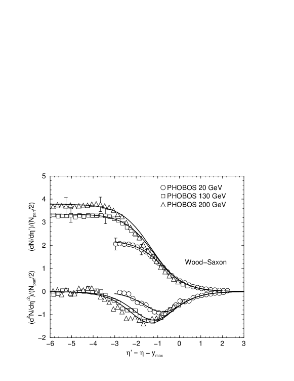
Figure 18: $\{{\chi_{f}},\sigma\}=\{1.32,0.694\}$ for 200 GeV, $\{1.20,0.681\}$ for 130 GeV and $\{0.77,0.619\}$ for 19.6 GeV. The limiting curve parameters are $\kappa_{0}=0.492$ and $1/\sigma_{0}=1.253$.

For large enough $({y_{\rm max}}-{\eta_{f}})/\sigma$,

$${1\over\sigma}\approx{1\over\sigma_{0}}(1+e^{-({y_{\rm max}}-{\eta_{f}})/\sigma_{0}})$$ (46)

ignoring terms of $O(e^{-2({y_{\rm max}}-{\eta_{f}})/\sigma_{0}})$. At an asymptotically high energy,

$$\lim_{{y_{\rm max}}\to\infty}\sigma=\sigma_{0}$$ (47)

Hence the limiting curve is given by

$$f_{U}(\eta^{\prime})=\kappa_{0}\,e^{-\eta^{\prime}/\sigma_{0}}$$ (48)

Fitting the $\eta>{y_{\rm max}}$ portion of $\sqrt{s}=19.6\,\hbox{\,GeV}$ data yields $1/\sigma_{0}=1.253$ and $\kappa_{0}=0.492$ as shown in Fig. 5. The height of the plateau and the total multiplicity can be now easily obtained from Eq.(30)

$$\left(dn\over d\eta\right)_{0} = {\kappa_{0}(1+e^{({y_{\rm max}}-{\eta_{f}})/\sigma})\over 1+e^{-{\eta_{f}}/\sigma}}$$ (49)

and

$$n_{\rm total}=2{\eta_{f}}\,\left({dn\over d\eta}\right)_{0}+O(e^{-{\eta_{f}}/\sigma})$$ (50)

The resulting $dn/d\eta$ and $d^{2}n/d\eta^{2}$ are shown in Fig. 18 together with PHOBOS data. Note that although fragmentation region universality is reasonably well described by the Wood-Saxon functions, the transition region universality is not. Again, we emphasize that it is the slope ($d^{2}n/d\eta^{2}$) that gives clearer criterion for the goodness of the description.

Unlike the previous case, the Wood-Saxon case has no separate ${\eta_{p}}$. This is because both the fragmentation and the transition behaves like an exponential $\sim e^{-|\eta-{\eta_{f}}|/\sigma_{0}}$ near ${\eta_{f}}$. Therefore the transition between the plateau and the limiting behavior happens within about $3\sigma_{0}$ around ${\eta_{f}}$. This fact also indicates that dynamics of the plateau and the dynamics of the fragmenation region does not decouple even at an asymptotically high $\sqrt{s}$.

This non-decoupling also allows us to put a severe condition on the transverse energy. To calculate the energy content of the plateau, we need to carry out an integral over the product of the Wood-Saxon and a hyperbolic cosine. This can be done, but the resulting form is not particularly illuminating. However, within the plateau we can approximate

$$E_{\rm plateau} \approx 2\left(dn\over d\eta\right)_{0}\left\langle m_{T}\right\rangle_{\rm pl.}\,\sinh({\eta_{f}})$$ (51)

Energy conservation demands that

$$\left\langle m_{T}\right\rangle_{\rm pl.}<{m_{N}\over\kappa_{0}}\,e^{-(1/\sigma-1)({y_{\rm max}}-{\eta_{f}})}$$ (52)

where we used Eq.(49). Since $\sigma<1$, this indicates that the average transverse energy in the plateau region must be a decreasing function of ${y_{\rm max}}$ if ${y_{\rm max}}-{\eta_{f}}$ is an increasing function of ${y_{\rm max}}$. This is an absurd result. One would expect that as $\sqrt{s}$ becomes larger, $\left\langle m_{T}\right\rangle_{\rm pl.}$ would also become larger or at least reach a limiting value, but not decrease. This, in our opinion, invalidates the Wood-Saxon description of $dn/d\eta$.

Nevertheless, it is instructive to also have the extrapolated Wood-Saxon result to LHC. For the Wood-Saxon form, we find that ${\chi_{f}}=1.32,1.20,0.77$ for $\sqrt{s}=200\,\hbox{\,GeV}$, $130\,\hbox{\,GeV}$, $20\,\hbox{\,GeV}$, respectively. These yield

$${y_{\rm max}}-{\eta_{f}}=\left\{\begin{array}[]{ll}0.59\,y_{\rm max}^{0.85}-0.68\,\ln{y_{\rm max}}&\ \ (\hbox{WS I})\\ -0.47+0.57\,y_{\rm max}^{0.69}&\ \ (\hbox{WS II})\end{array}\right.$$ (55)

The results for LHC are tabulated in Table 2. The values of $(dn/d\eta)_{0}$ and $n_{\rm total}$ are comparable to the saturation model (K & L) values in Table 1. Also one can easily see in Fig. 19 that the limiting fragmentation curve followed by the Wood-Saxon functions is not the same as the one followed by the interpolating-exponential ones.

	${y_{\rm max}}-{\eta_{f}}$	$(dn/d\eta)_{0}$	$n_{\rm total}$
WS I	2.3	10.6	130
WS II	2.1	8.5	110

Table 2: Predictions for LHC central collisions using the Wood-Saxon form. We set $\sqrt{s}=5.5\,\hbox{TeV}$ and Pb+Pb.

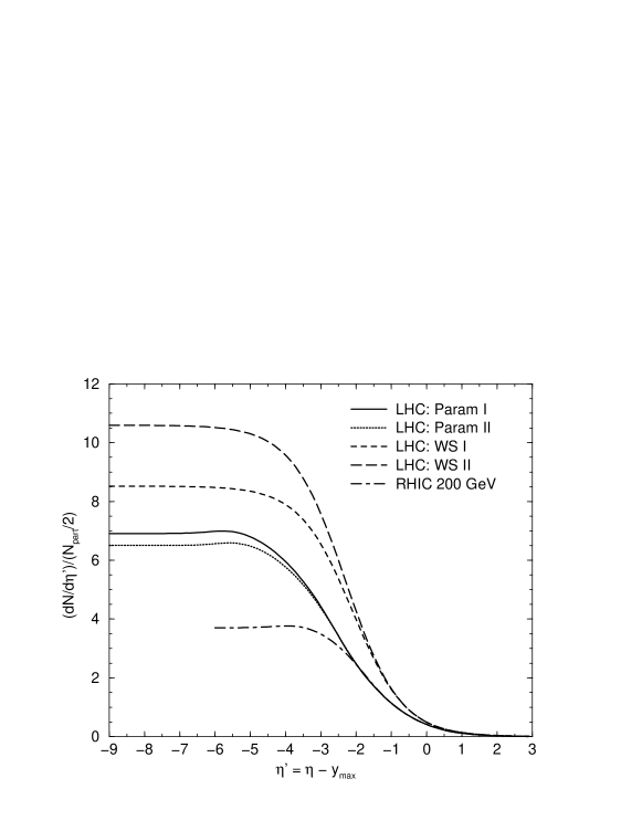
Figure 19: Predictions for central collisions at LHC. Also shown are parametrized RHIC 200 result. We set $\sqrt{s}=5.5\,\hbox{TeV}$ and Pb+Pb for LHC.