Nuclear Structure, Random Interactions and Mesoscopic Physics

Abstract

Standard concepts of nuclear physics explaining the systematics of ground state spins in nuclei by the presence of specific coherent terms in the nucleon-nucleon interaction were put in doubt by the observation that these systematics can be reproduced with high probability by randomly chosen rotationally invariant interactions. We review the recent development in this area, along with new original results of the authors. The self-organizing role of geometry in a finite mesoscopic system explains the main observed features in terms of the created mean field and correlations that are considered in analogy to the random phase approximation.

1 Introduction

It became a common place to claim that the basic facts of the nuclear ground state systematics, namely that all even-even nuclei have ground state spin $J_{0}=0$ and the lowest possible isospin $T_{0}=T_{{\rm min}}$, are due to the fundamental properties of residual nucleon-nucleon forces. The pairing phenomenon was known, in particular through the mass formula, from the beginning of nuclear spectroscopy. It was formulated by Racah in an elegant form with the use of the seniority quasispin formalism [1, 2]. The predictions of the simple shell model by Mayer and Jensen [3] would be uncertain for all nuclei, except magic ones and those with one particle or one hole on top of the magic core, if the pairing would not allow one to guess that the nuclear ground state spin in odd-$A$ nuclei is determined by the last unpaired nucleon. A. Bohr, Mottelson and Pines [4] found a profound analogy of nuclear pairing to superconducting pair correlations of electrons in metals, and Belyaev in his seminal paper [5] demonstrated how the pairing interaction creates correlations that modify not only the ground state energy but all single-particle and collective properties of low-lying nuclear states, in a good agreement with observed trends [6].

Following the advances in experiments and theory towards nuclei far from stability, the interest to pairing has recently increased. The pairing correlations play a decisive role in determining the nuclear drip-line; many nuclides can be stable only due to the pairing correlations between the outermost loosely bound nucleons. The pairing interaction is an inalienable and very important part of all modern shell model versions [7].

Therefore an unexpected observation by Johnson, Bertsch and Dean [8] was met with great interest and immediately put under the microscope of various tests. They noticed that even randomly taken two-body forces acting between the fermions in a restricted Hilbert space of few single-particle orbitals lead to the statistical predominance of the ground state spin $J_{0}=0$. The broad discussion that followed this discovery revealed that similar phenomena take place for interacting bosons as well. The natural questions arise: do we understand well the physics generated by random interactions under constraints of rotational symmetry and what is the reason for empirical regularities in nuclei? The problem is not limited to nuclear physics. Atomic clusters, particles in the traps, quantum dots and disordered systems, such as quantum spin glasses, are just a few examples where the same questions are to be answered.

From a more general theoretical viewpoint related to many-body quantum chaos [9, 10, 11], we deal with closed mesoscopic systems that generically display chaotization of motion due to intrinsic interactions. In the absence of a heat bath and external disorder, the interactions play the role of a randomizing or thermalizing factor. They create a very complicated structure of the eigenstates. However, the presence of exact symmetries (rotational, time-reversal, parity, isospin) leads to non-vanishing correlations between the classes of states with different exact quantum numbers since they are governed by a single deterministic (even if randomly picked) Hamiltonian with a relatively small number of parameters. Such correlations bring a new, hardly discussed before, element to theory of quantum chaos.

Below we describe the problem more in detail following the main ideas proposed for explanation by various authors. We show that a conventional notion of a mean field created by the interaction removes the main puzzling features of the problem and puts the whole story on a clear track. Of course, the open questions still remain leaving the room for future exciting studies.

2 Two-body interactions in an isolated many-body system and many-body quantum chaos

2.1 Hamiltonian

Our starting point is a standard shell-model approach to a many-body problem. $N$ particles are interacting through two-body forces within Hilbert space that is built on a certain number of single-particle orbitals. We label the single-particle states as $|1)$, incorporating all necessary quantum numbers in the unified label 1. Using the single-particle basis diagonalizing the independent particle part, the general Hamiltonian of the system can be written as

$$H=\sum_{1}\epsilon_{1}a^{\dagger}_{1}a_{1}+\frac{1}{4}\sum_{1234}V(12;34)a^{\dagger}_{1}a^{\dagger}_{2}a_{3}a_{4},$$ (1)

where we introduced the creation and annihilation operators with usual commutation (anticommutation) rules for bosons (fermions). The interaction matrix elements $V(12;34)$ are correspondingly symmetrized (antisymmetrized) with respect to permutations $1\leftrightarrow 2$ and $3\leftrightarrow 4$. Assuming time-reversal invariance, we can consider all matrix elements real. The restriction to two-body forces (“rank” of the interaction $r=2$) is not significant as long as the total particle number $N\gg r$, and can be removed. Note that the general form (1) does not explicitly carry any conservation law except for the particle number. Later we consider the requirements of rotational (or isospin) invariance.

Two physical formulations can be considered in parallel. In application to a realistic system, the Hamiltonian is derived from more general theory (for example, for nuclei it can be based on meson theory or quark models) or built empirically with the parameters, $\epsilon_{1}$ and $V(12;34)$, adjusted to experimental data. One can also consider ensembles of Hamiltonians that satisfy the requirements of Hermiticity and quantum statistics but the parameters, or part of them, are treated as random variables taken from some distribution. The explicitly introduced randomness of the Hamiltonian keeping the same form as that of actual mesoscopic systems was used with the purpose to bring the global description in terms of random matrices near to physical reality. It turns out that the local spectral statistics, starting from sufficiently high level density, are universal. They express generic properties of many-body quantum chaos (plus the assumption of time reversal invariance) and do not depend on the details of the interaction. Below we first characterize these universal features and then turn to the ground state problem.

2.2 Ensemble of random interactions

The studies of the random two-body interactions go back to Wigner-Dyson random matrix theory, see [12] and references therein. This stage of development was thoroughly reviewed by Brody et al. in Ref. [13]; see also the latest review [14]. The two-body random ensemble, TBRE [15, 16], in contrast to full canonical (Gaussian Orthogonal, GOE, or Gaussian Unitary, GUE) ensembles [17], considers matrices in many-body Hilbert space, where nonzero off-diagonal matrix elements link the independent particle states that can be connected by two-body processes but not constrained by any conservation laws, except for the symmetry dictated by the particle statistics. These matrix elements are taken in the TBRE as uncorrelated and normally distributed real random quantities. More general embedded ensembles [18] can be considered with $r$-body forces [19] for $r<N$; the case $r=N$ with a simultaneous interaction of all particles returns to the full GOE. The angular momentum conservation was, as a rule, ignored because of severe mathematical difficulties [13].

We see essential new properties of the TBRE as compared to the canonical random matrix ensembles. (i) The orthogonal, or unitary, invariance of the statistical distribution of random matrix elements is lost. (ii) The natural basis is that of independent particle configurations where only configurations that differ by not more than the occupancies of a pair of orbitals in the initial and final states can be connected by a single-step interaction. In this basis the many-body Hamiltonian matrix is sparse. (iii) The nonzero matrix elements of this matrix are strongly correlated. Indeed, a given two-body scattering process may occur on the background of many different spectator configurations of remaining particles; all many-body matrix elements in those cases are equal regardless of a random or deterministic character of the two-body interaction.

Before the work [8], the studies of the TBRE did not consider the consequences of rotational invariance so that the single-particle levels did not carry any additional quantum numbers being fully characterized by their energy. The most important conclusion of these studies was the “chaotic” character of local spectral statistics, essentially the same as predicted for the GOE in spite of a very different distribution of many-body matrix elements. Many results are insensitive to the exact form of the distribution function of random two-body matrix elements that can differ from the Gaussian still remaining symmetric with respect to the sign. It was established [20] that the global (“secular”) behavior of the level density in the given finite Hilbert space of a certain number of single-particle orbitals is close to Gaussian for $N>r$ while for $N=r$ it tends to the semicircle typical for the GOE or GUE. There are only few analytical results for the TBRE and its modifications [18], although significant numerical work has been done.

2.3 Complexity of many-body states

The detailed shell model studies for complex atoms [9] and nuclei [10] showed that realistic forces, Coulomb for atoms and semiempirical effective nucleon-nucleon interactions for nuclei, generate the local spectral statistics well described by the GOE and TBRE within each class of many-body states with fixed exact quantum numbers. Considering the dependence on the interaction strength, the chaotic statistics of nearest level spacings and the so-called $\Delta_{3}$ statistics of level number fluctuations emerge when the interparticle interactions are turned on with their strength still much weaker than the realistic value. This happens without any randomness in the Hamiltonian, in spite of correlations due to the two-body character of the forces and the fact that the realistic distributions of the many-body matrix elements are generically close to exponential rather than Gaussian [10]. The mechanism of spectral chaotization is provided by multiple avoided crossings of levels inside a fixed symmetry class.

As the interaction strength increases beyond threshold for onset of spectral chaos, and level dynamics with less frequent crossings loses its turbulent character, the main ongoing process is the growth of complexity of the eigenfunctions. The important question here is how one can quantify the degree of complexity of an individual wave function. The specification of a wave function is always related to a certain basis $|k\rangle$. In the eigenbasis of the Hamiltonian, each eigenfunction has just one component that obviously indicates the absence of complexity. In the above mentioned process of switching on interaction, it is natural to refer all eigenstates to the original basis of noninteracting particles and follow the gradual increase of complexity measured by the number of significant components in the wave function. This choice of the reference basis is also singled out by many-body physics. In a realistic system of the type we are interested in, the single-particle structure is determined by the self-consistent field due to all particles. The mean field embodies the most regular effects of the interaction. The residual interactions already do not contain such average components. Therefore one can think of the mean field basis as the best choice for separating regular and chaotic aspects brought in by the interaction [21].

The degree of complexity of an eigenstate $|\alpha\rangle$ with respect to the reference basis $|k\rangle$ can be quantified with the help of Shannon information entropy [22, 23, 10]. If the eigenfunction is given by the normalized superposition

$$|\alpha\rangle=\sum_{k}C^{\alpha}_{k}|k\rangle,$$ (2)

information entropy of the state $|\alpha\rangle$ in the basis $|k\rangle$ is defined in terms of the weights $w^{\alpha}_{k}=|C^{\alpha}_{k}|^{2}$ as

$$I_{\alpha}=-\sum_{k}w^{\alpha}_{k}\ln w^{\alpha}_{k}.$$ (3)

As the interaction strength increases, information entropy grows from zero in principle being able to reach the limit of $I_{{\rm max}}=\ln d$, where $d$ is the space dimension. This maximum possible value can be realized for the fully delocalized function with all equal weights $w^{\alpha}_{k}=1/d$. In the GOE the average value of $I_{\alpha}$ is lower than this limit, $I_{{\rm GOE}}=\ln(0.48d)$, because of the requirements of orthogonality of different eigenstates.

The shell model analysis [23, 10] shows that information entropy in all symmetry classes grows smoothly with the interaction strength and in the middle of the spectrum gets close to the $I_{{\rm GOE}}$. With the interaction strength artificially increased beyond its realistic value, one can reach the GOE limit uniformly in excitation energy [24, 10]. It is important that for the realistic, and therefore consistent with the mean field, interaction strength information entropy $I_{\alpha}$ is a smooth monotonously increasing to the middle of the spectrum function of excitation energy $E_{\alpha}$. This allows one to treat information entropy as a thermodynamic variable and build up the corresponding temperature scale [24, 10, 11] avoiding any reference to a heat bath or Gibbs ensemble. Thus, one can consider thermodynamics of a closed mesoscopic system based on typical properties of individual quantum states.

The physical foundation for that is given by the chaotic mixing of states as a result of the strong interaction at a high level density. This mixing makes statistical properties of closely located states uniform (thereby the question by Percival [25] on a generic relation between the complicated neighboring states is solved - “the states look the same”) and guarantees that macroscopic observables do not depend on the exact population of adjacent microscopic states and the corresponding phase relationships. This is exactly what is needed for the statistical description. Such considerations shed new light on a problem of justification of the thermodynamic approach for closed mesoscopic systems.

The quantity $d_{\alpha}=\exp(I_{\alpha})/0.48$ can be interpreted as an effective number of significant (“principal”) components of the wave function, or its localization length. The components $C_{k}^{\alpha}$ of a complicated wave function $|\alpha\rangle$ on average are uniformly distributed over a sphere of dimension $d_{\alpha}$. The fully uniform distribution on a $d$-dimensional sphere is restricted only by the normalization,

$$P_{d}(C_{1},...,C_{d})=\frac{\Gamma(d/2)}{\pi^{d/2}}\,\delta(\sum_{k=1}^{d}w_{k}-1),$$ (4)

which leads to the distribution function of any chosen component $C$

$$P_{1}(C)=\frac{\Gamma(d/2)}{\sqrt{\pi}\Gamma((d-1)/2)}\,(1-w)^{(d-3)/2},$$ (5)

where, as in eq. (4), $w=C^{2}$. In the asymptotic limit of large $d$, this distribution goes to the Gaussian. The square of the amplitude has a distribution

$$P_{1}(w)=\frac{\Gamma(d/2)}{\sqrt{\pi}\Gamma((d-1)/2)}\,\frac{1}{\sqrt{w}}\,(1-w)^{(d-3)/2}$$ (6)

that goes to the Porter-Thomas ($\chi^{2}$) distribution for large $d$. The realistic distributions of the components in the nuclear shell model [26, 10], except for the lowest and the highest states, are close to these predictions with local values of $d_{\alpha}$ smoothly changing along the spectrum, The strength distribution (6) along with the nearest level spacing distribution can serve as an experimental means for recovering the strength missing in the background of experiments that cannot resolve the invisible fine structure [27].

The complexity measure $I_{\alpha}$ or $d_{\alpha}$ gives a tool for estimating matrix elements of simple operators between a simple and complicated state or between two complicated states. In both cases, the typical reduction of the matrix element compared to that between two simple (let say, noninteracting) states is given by the factor $1/\sqrt{d}$ if one assumes that the two complex states have a similar degree of complexity. Since the corresponding level density, which determines energy denominators, increases on average $\propto d$, we come to the statistical enhancement of perturbations, $\propto\sqrt{d}$, in the region of many-body quantum chaos [28]. In light nuclei this enhancement can be seen directly in shell model calculations [29]. Remarkable examples are given by the strong enhancement of weak interactions in nuclear neutron resonances (parity violation in polarized neutron scattering [30, 31, 32] and fragment asymmetry in fission by polarized neutrons [33, 34]). Here again we see that statistical regularities in a mesoscopic system coexist with the opportunity to reveal, both theoretically and experimentally, properties of individual quantum states.

2.4 Chaos and thermalization

Another aspect of the same problem is the possibility to describe complicated eigenstates in the standard statistical language of single-particle occupation numbers. It was noticed, both for atoms [9], and nuclei [24, 10, 11], that expectation values of the occupation numbers $n_{j}$ of the mean field orbitals are close to what would be predicted by Fermi-Dirac statistics. Effective temperatures $T_{\alpha}$ extracted for individual states $|\alpha\rangle$ are in good correspondence with thermodynamic temperature determined by the level density as well as with the information temperature found from Shannon entropy. This shows that one can successfully use the notions of Fermi-liquid theory modeling the system as a gas of quasiparticles not only near the ground state, as it is usually assumed (in nuclei just in this region the description has to be modified because of pairing correlations [35]), but practically at any excitation energy below decay threshold. The finite lifetime of quasiparticles is simply translated into statistical occupation factors different from 0 and 1 and smoothly changing along the spectrum. The analytical description of the process of equilibration was given by Flambaum, Izrailev and Casati [36], and Flambaum and Izrailev [37] in the framework of the TBRE.

We need again to stress that information entropy is capable to characterize the degree of complexity only relative to a reference basis. This can be considered as an advantage of information entropy as a measuring tool since we are able to discover relations between the eigenbasis and various reference choices. The special role of the self-consistent mean field basis is now seen in the consideration of the occupation numbers defined with respect to this basis that forms a skeleton supporting all complications induced by the interaction. The equilibrating factor is the interparticle interaction rather than a heat bath. For the interaction of rigid spheres, which is known to generate chaotic dynamics, it was shown rigorously [38] that the equilibrium momentum distribution is that of Boltzmann, Bose-Einstein or Fermi-Dirac depending on the statistics of particles even if the interaction cannot be reduced to gaseous rare collisions. In realistic cases the interaction strength is in accordance with the parameters of the mean field. In the case of artificially enhanced interaction, all states go to the GOE limit of complexity, and the single-particle thermometer is not capable of resolving the spectral evolution [24, 10].

The description with the aid of information entropy does not take into account any phase correlations between the components of an eigenfunction. In a sense it gives a delocalization measure [10, 18] of the given state in the original basis of noninteracting particles. It cannot distinguish between an incoherently mixed chaotic state and collective state that is a regular superposition of many basis states with certain phase relationships. The information approach may be also inadequate for an unstable mean field or a phase transition occurring at some temperature (excitation energy). Here another way of characterizing the individual quantum states may be useful [39]. One can look at the response of a given state $|\alpha\rangle$ to external noise described by random parameters $\lambda$ in the Hamiltonian. The averaging over $\lambda$ determines the density matrix

$$\rho^{\alpha}_{kk^{\prime}}=\langle C^{\alpha}_{k}(\lambda)C^{\alpha\ast}_{k^{\prime}}(\lambda)\rangle_{{\rm av}}$$ (7)

that allows one to define von Neumann entropy

$$S_{\alpha}=-{\rm Tr}\{\rho^{\alpha}\ln(\rho^{\alpha})\}.$$ (8)

In contradistinction to information entropy, this quantity, that may be called invariant correlational entropy (ICE), does not depend on the choice of representation and takes into account correlations between the amplitudes of the wave function.

The ICE is very sensitive to quantum phase transitions. If the random parameter $\lambda$ fluctuates around the phase transition point, the strong variation of the structure of the state gives rise to a peak in the ICE as was shown in the interacting boson model (IBM) [40] and in the realistic shell model [41]. One can notice also a common physical aspects shared by the ICE and the notion of fidelity extensively studied recently in considerations of quantum dynamics related to quantum echo, decoherence, Zeno effect and quantum computing, see for example [42, 43, 44].

3 Rotational invariance

3.1 Role of symmetries

From the very beginning of studies of random matrices and quantum chaos, the crucial influence of global symmetries was repeatedly stressed by many authors. Random matrix ensembles make averaging over all Hamiltonians in a given universality class [12]. The classes are fully determined by the fundamental symmetries as Hermiticity, both for GOE and GUE, and time-reversal invariance (for GOE). The additional requirement for the canonical Gaussian ensembles is the invariance of the distribution of matrix elements under orthogonal or unitary basis transformations. This last demand expresses the limiting property of extreme chaos and brings at our disposal the necessary reference point, against which we can look at the realistic systems with their specific deviations from this limit. The ensembles as TBRE do not obey this requirement but this does not influence the local spectral statistics. In addition an exact permutational symmetry for fermions or bosons is also imposed here.

Self-sustaining mesoscopic systems reveal other exact symmetries, first of all rotational symmetry (in the absence of external fields). As a result, any eigenstate is a member of a degenerate rotational multiplet $|JM\rangle$ with total spin $J$ and its projection on the laboratory quantization axis $J_{z}=M$. The classes of states with different quantum numbers of $J$ and $M$ are not mixed, and one can study the onset of chaos, spectral characteristics, complexity of wave functions and so on for each class separately. The situation is similar, for example, to the Sinai billiard, where the studies responsible for a hypothesis [45] of the correspondence between quantum level statistics and classical chaos can be tested using one octant of the billiard and continuing wave functions to the entire area according to the symmetry class. Combining states of various classes into a common spectrum, one comes to the Poissonian level statistics [46, 13]. To the best of our knowledge, correlations between the states of different exact symmetry in the same billiard were not studied.

At the same time, serious efforts were applied to the problems of approximate symmetries, onset of chaos along with destruction of symmetry, transition from the GOE to GUE due to violation of time-reversal invariance by the magnetic field or $T$-odd nuclear forces, intermediate spectral statistics and so on [14]. The example most relevant to nuclear structure is given by the isospin invariance [47]. The classes of nuclear states with different isospin are mixed by electromagnetic interactions and strong forces violating charge symmetry, and this can be seen in transition probabilities and reaction amplitudes. In the shell model versions with exact isospin conservation and without weak interactions, the classes of states are characterized by exact quantum numbers $J^{\pi}T$.

The common Hamiltonian that governs nuclear dynamics certainly establishes correlations between the states of different classes even if they belong to the region of quantum chaos. One can imagine, for instance, a deformed system with extremely chaotic many-body dynamics inside. Nevertheless, the rotational invariance guarantees the existence of the rotational branch of the excitation spectrum with energy $E_{J}$ at least approximately given by $AJ(J+1)$. In a macroscopic system, this would be a continuous Goldstone mode that emerges because of the spontaneous orientational symmetry breaking by the choice of the body-fixed frame; in a finite system it is simply a rotational band, or, for a chaotic system, “compound band” as suggested by Mottelson [48]. Thus, we obtain a clear correlation between the states of the same band in different $J$-classes. The intrinsic structures of these states should also be close. In a sense, this might even be a classical rigid body with microscopic quantum chaos of interacting constituents.

3.2 Geometric chaoticity

Consider a finite many-body system with exact angular momentum conservation. The total spin of the system,

$${\bf J}=\sum_{a}{\bf j}_{a},$$ (9)

is built up of spins of individual constituents. As a number of particles grows, so does the number of independent ways of building a many-body state of a given total spin $J$. This number determines the dimension of a given $J$-class, $d_{J}$; a similar construction is necessary for a total isospin $T$. Those independent combinations correspond to various recouplings of spins in the process of constructing the full state:

$$\{[(j_{1}j_{2})j_{12}j_{3}]j_{123}j_{4}\}j_{1234}...J.$$ (10)

Different paths to the same values of $J$ can be distinguished by high $nj$-symbols or coefficients of fractional parentage.

In the shell model, even with a particle number of the order of 10, the number of different paths, eq. (10), is large, and the resulting products of many consecutive Clebsch-Gordan coefficients (CGC) determine the orthogonal combinations within the same class. Let us, for example, look at the class $J=0$ in a system of an even particle number. We can start with a simple state of seniority $s=0$, when we couple particles pairwise to $j_{12}=j_{34}=...0$ (to guarantee the full permutational symmetry it is more convenient to use the pair operators in secondary quantization, as we do below). Here all CGC are trivial, and the state has a very regular structure. Each new state should be orthogonal to all previous ones, so that at some point we have to employ another combination (a closed loop or few loops of vectors ${\bf j}_{a}$) that proceeds through different intermediate stages. At a sufficiently large dimension, the majority of paths look as a random walk process of vector coupling. This source of randomness we call geometrical chaoticity.

The property of geometrical chaoticity was practically used long ago by Bethe [49], see also [50], to derive the partial nuclear level density $\rho(E;J)$ for a given angular momentum in the model of noninteracting fermion gas. Assuming that the projections $j_{z}=m$ of particle spins are coupled into the total projection $M$ in a random walk process, one can apply the central limit theorem and come to the Gaussian probability $w(M)$ of a given value of $M$ with zero mean and the variance

$$(\Delta M)^{2}=N\langle m^{2}\rangle,$$ (11)

expressed in terms of the (energy-dependent) number $N$ of active fermions (particles and holes) and average single-particle value of $m^{2}$ in space of available orbitals. The level density with given $M$ is then given by $\rho(E;M)=\rho(E)w(M)$, where $\rho(E)$ is the total level density. Using the standard trick, one can get the approximate expression for the multiplicity $d_{J}$ of states with given spin $J$,

$$\frac{d_{J}}{d}=w(J)-w(J+1)\approx\frac{2J+1}{2\sqrt{2\pi}(\Delta M)^{3}}e^{-J(J+1)/2(\Delta M)^{2}}.$$ (12)

This result, invalid for the largest values of $J$, shows that the maximum of the multiplicity is near $J=\Delta M-1/2$. From eq. (11) we see that it grows $\propto\sqrt{N}$.

Regrettably, it is very hard to develop a statistical theory for a random process with quantized vectors as ${\bf j}_{a}$ that are coupled not algebraically. This would be equivalent to developing statistical theory of fractional parentage coefficients. In spite of various attempts and some useful results that can be extracted from works by Wigner [51], Ponzano and Regge [52] and others [53, 54], such theory still does not exist.

The reality of geometric chaoticity is clearly seen in the nuclear shell model [10]. Prior to any diagonalization, one can derive important characteristics of the energy spectrum directly from the Hamiltonian matrix. A basis state $|JT;k\rangle$ of independent particles projected onto certain values of spin and isospin is a superposition of the stationary states $|JT;\alpha\rangle$ with the same real amplitudes $C^{\alpha}_{k}$ that determined the composition of the eigenstate in eq. (2). The weights $w^{\alpha}_{k}$ define the strength function $F_{k}(E)$ of the simple state $|JT;k\rangle$ according to

$$F_{k}(E)=\sum_{\alpha}w^{\alpha}_{k}\delta(E-E_{\alpha}),$$ (13)

where $E_{\alpha}$ are energies of the eigenstates. The strength function (since $\sum_{k}F_{k}(E)=\rho(E)$, it is called local density of states in condensed matter theory, where the basis states $|k\rangle$ are localized ones) determines the time evolution of the state $|k\rangle$ prepared at the initial moment. The centroid of the strength function $F_{k}(E)$ is given by the diagonal matrix element of the Hamiltonian, $H_{kk}$. The energy dispersion $\sigma_{k}$ of the state $|JT;k\rangle$ can be found as

$$\sigma^{2}_{k}=\langle k|(H-H_{kk})^{2}|k\rangle=\sum_{l\neq k}H_{kl}^{2},$$ (14)

the sum of all off-diagonal matrix elements in the $k^{{\rm th}}$ row of the Hamiltonian matrix. A remarkable fact is that in a given shell model class $(JT)$ the dispersions $\sigma_{k}$ are nearly constant, $\sigma_{k}\approx\bar{\sigma}$, for all states $|JT;k\rangle$. This equilibration for noninteracting particles comes only from the $JT$-projection, and therefore is the direct output of geometric chaoticity that accompanied the projection algorithm. Parenthetically we can mention that the constant magnitude of the dispersion (14) is important for determination of the spreading width of the strength function [55] that approaches the limit of $2\bar{\sigma}$ in the case of strong fragmentation.

3.3 Rotationally invariant two-body Hamiltonian

Now we explicitly introduce the requirements of rotational invariance in the Hamiltonian (1), both for single-particle states and the interaction. We assume spherical symmetry of the mean field with orbitals characterized by the angular momentum $j$, its projection $j_{z}=m$, and isospin projection $\tau_{3}$. For definitiveness we consider fermions with isospin 1/2 and assume that every value of $j$ appears only once. The Hamiltonian of the system is determined by the set of single-particle energies $\epsilon_{j}$ that, under conditions of rotational and isospin invariance, do not depend on $m$ and $\tau_{3}$, and by the interaction that preserves the total angular momentum $L$ and total isospin $t$ of the interacting pair. The eigenstates of the Hamiltonian have exact quantum numbers of total angular momentum, $J$ and $J_{z}=M$, and total isospin, $T$ and $T_{3}$.

The most general form of the two-body interaction under such conditions is

$$H_{int}=\sum_{L\Lambda,tt_{3};\{j\}}V_{Lt}(j_{1}j_{2};j_{3}j_{4})P^{\dagger}_{L\Lambda,tt_{3}}(j_{1}j_{2})P_{L\Lambda,tt_{3}}(j_{3}j_{4}).$$ (15)

Here we use the pair annihilation and creation operators for each $Lt$-pair channel,

$$P_{L\Lambda,tt_{3}}(j_{1}j_{2})=\frac{1}{\sqrt{1+\delta_{j_{1}j_{2}}}}[a_{j_{1}}a_{j_{2}}]_{L\Lambda,tt_{3}},$$

$$P^{\dagger}_{L\Lambda,tt_{3}}(j_{1}j_{2})=\frac{1}{\sqrt{1+\delta_{j_{1}j_{2}}}}[a^{\dagger}_{j_{2}}a^{\dagger}_{j_{1}}]_{L\Lambda,tt_{3}},$$ (16)

where the vector coupling with the appropriate CGC to the total rotational ($L\Lambda$) and isospin ($tt_{3}$) quantum numbers of the pair is implied, Fig. 1. One can also remove isospin invariance taking different values for proton and neutron single-particle levels and interaction matrix elements but still preserving angular momentum conservation.

Figure 1: The diagram of the two-body interaction in particle-particle and particle-hole channels characterized by the total spins, $L$ and $K$, respectively.

In this formulation, the numerical parameters of the Hamiltonian are, apart from the single-particle energies, the interaction amplitudes $V_{Lt}$ that do not depend on projections $\Lambda$ and $t_{3}$. The number $k$ of these amplitudes is typically much smaller than the number $d_{JT}$ of levels in the $JT$-class (the classes with the largest possible values of $J$ and $T$ might be exceptional in this respect). Thus, the well studied nuclear $sd$ shell model includes $d_{5/2},s_{1/2}$ and $d_{3/2}$ orbitals for neutrons and protons. This model is completely defined by three single-particle energies and 63 interaction matrix elements $V_{Lt}$ while, for example, with 12 valence fermions, there are 839 states in the class with lowest quantum numbers $JT=00$ [10], the largest class in this model appears with $JT=31$ and has $d_{JT}=6706$.

It is always possible to recouple the creation and annihilation operators from the particle-particle channel used in eqs. (1) and (15) to the particle-hole channel, see Fig. 1, where the Hamiltonian would have the multipole-multipole structure $\{[a^{\dagger}a]_{K}[a^{\dagger}a]_{K}\}_{00}$ with the spin $K$ of the particle-hole pairs; the similar recoupling is performed for isospins. The corrections to the orbital energies (one-body terms) appear in this process. The transformation can be done in two ways which correspond to the crossing transition from the $s$-channel to $t$- and $u$-channels in quantum field theory. It is important to stress that, although not seen immediately, the number of parameters is the same in different channels because of the permutational symmetry of identical particles, as will be shown better in the next subsection.

The typical class dimensions of few hundred up to few thousand make the nuclear shell model a perfect tool for studying the exact solution of a many-body problem. With dimensions of this size, the diagonalization is straightforward and we obtain all individual eigenfunctions while the statistical regularities are already clearly pronounced. Thus, we are in a typical realm of mesoscopic physics. Again we stress that all classes of states are described by the same matrix elements and therefore have to be correlated.

The particle-particle interaction channel with $L=0$ and $t=1$, when $j_{1}=j_{2}$ and $j_{3}=j_{4}$, represents conventional isospin-invariant isovector pairing. This component of the interaction is, as a rule, considered to be responsible for the main pairing effects in binding energy. It is possible that around the $N=Z$ line the isoscalar pairing, $t=0$, is important, especially in nuclei far from stability; for classification of various types of pairing see, for example [56] and references therein. According to the generalized Pauli principle for a two-nucleon system, the symmetries in spin-spatial variables and in isospin are complementary. The symmetry relation for the pair operators (16) reads

$$P_{L\Lambda,tt_{3}}(j_{1}j_{2})=(-)^{j_{1}+j_{2}+L+t}P_{L\Lambda,tt_{3}}(j_{2}j_{1}).$$ (17)

In particular, for $j_{1}=j_{2}$, only even values $L=0,2,...,2j-1$ are allowed for $t=1$ (or for identical fermions without isospin) while $t=0$ requires the odd values $L=1,3,...,2j$. With time reversal invariance, the parameters $V_{Lt}$ can be chosen real.

3.4 Single $j$-level

Here we give the formalism for the simplest fermionic space, namely that of $\Omega=2j+1$ single-particle states $|jm)$ of a single $j$-level for one kind of particles. With this simplification, it will be possible to see the core of the problem. In this case the mean field part is just a constant proportional to the particle number, and the Hamiltonian takes the form

$$H=\epsilon N+\sum_{L}V_{L}\sum_{\Lambda}P^{\dagger}_{L\Lambda}P_{L\Lambda},$$ (18)

where the pair operators are defined in terms of the $3j$-symbols as

$$P^{\dagger}_{L\Lambda}=\frac{1}{\sqrt{2}}\sum_{m_{1}m_{2}}\sqrt{2L+1}(-)^{L-\Lambda}\left(\begin{array}[]{ccc}j&L&j\\ m_{1}&-\Lambda&m_{2}\end{array}\right)a^{\dagger}_{1}a^{\dagger}_{2}.$$ (19)

Only even $L$ pairs are present in eq. (18) so that the number of independent interaction parameters $V_{L}$ is $k=j+1/2$; all unnecessary labels are omitted.

We define the multipole operators in the particle-hole channel, Fig. 1, as

$$M_{K\kappa}=\sum_{m_{1}m_{2}}(-)^{j-m_{1}}\left(\begin{array}[]{ccc}j&K&j\\ -m_{1}&\kappa&m_{2}\end{array}\right)a^{\dagger}_{2}a_{1}.$$ (20)

Here any integer value of $K$ from 0 to $2j$ is allowed. The Hermitian conjugation gives

$$M^{\dagger}_{K\kappa}=(-)^{\kappa}M_{K-\kappa}.$$ (21)

The special important cases are the particle number operator

$$N=\sum_{m}a^{\dagger}_{m}a_{m}=\sqrt{\Omega}\,M_{00},$$ (22)

and the angular momentum (in spherical components)

$$J_{\kappa}=\sum_{mm^{\prime}}(m|j_{\kappa}|m^{\prime})a^{\dagger}_{m}a_{m^{\prime}}=\sqrt{j(j+1)\Omega}\,M_{1\kappa}.$$ (23)

The alternative, particle-hole, form of the Hamiltonian is

$$H=\tilde{\epsilon}N-\frac{1}{2}\sum_{K}\tilde{V}_{K}\sum_{\kappa}M^{\dagger}_{K\kappa}M_{K\kappa},$$ (24)

where the single-particle energy is renormalized,

$$\tilde{\epsilon}=\epsilon+\frac{1}{2\Omega}\sum_{K}\tilde{V}_{K},$$ (25)

and the interaction parameters are transformed according to

$$\tilde{V}_{K}=(2K+1)\sum_{L}(2L+1)\left\{\begin{array}[]{ccc}j&j&L\\ j&j&K\end{array}\right\}V_{L}.$$ (26)

Inversely,

$$V_{L}=\sum_{K}\left\{\begin{array}[]{ccc}j&j&K\\ j&j&L\end{array}\right\}\tilde{V}_{K}.$$ (27)

Since a reversible algebraic transformation cannot increase the number of independent parameters, there should exist constraints that reduce the number of independent constants $\tilde{V}_{K}$ from $2j+1$ to the number $k=j+1/2$ of the original parameters $V_{L}$. Indeed, the particle-hole amplitudes $\tilde{V}_{K}$ are interrelated through

$$\tilde{V}_{K}=(2K+1)\sum_{K^{\prime}}(-)^{K+K^{\prime}}\left\{\begin{array}[]{ccc}j&j&K\\ j&j&K^{\prime}\end{array}\right\}\tilde{V}_{K^{\prime}}.$$ (28)

These relations expressing the symmetry of recoupling between the $t$- and $u$-channels are important for the dynamics of the model. They were discussed more in detail by one of the authors [57]. In particular, we note the results for the pairing interaction, $L=0$,

$$V_{0}=-\frac{1}{\Omega}\sum_{K}(-)^{K}\tilde{V}_{K},$$ (29)

and monopole interaction, $K=0$,

$$\tilde{V}_{0}=-\frac{1}{\Omega}\sum_{K}\tilde{V}_{K}.$$ (30)

To conclude this section, we write down the commutator algebra of the pair and multipole operators (we use the abbreviation $g_{K}=\sqrt{2K+1}$),

$$[P_{L^{\prime}\Lambda^{\prime}},P^{\dagger}_{L\Lambda}]=\delta_{LL^{\prime}}\delta_{\Lambda\Lambda^{\prime}}+2\sum_{K\kappa}g_{K}^{2}X^{LL^{\prime};K}_{\Lambda\Lambda^{\prime}\kappa}M^{\dagger}_{K\kappa};$$ (31)

$$[P^{\dagger}_{L\Lambda},M_{K\kappa}]=2\sum_{L^{\prime}\Lambda^{\prime}}X^{LL^{\prime};K}_{\Lambda\Lambda^{\prime}\kappa}P^{\dagger}_{L^{\prime}\Lambda^{\prime}};$$ (32)

$$[M^{\dagger}_{K\kappa},M_{K^{\prime}\kappa^{\prime}}]=\sum_{S\sigma}[1-(-)^{K+K^{\prime}+S}]\frac{g_{S}^{2}}{\sqrt{g_{K}g_{K^{\prime}}}}X^{KK^{\prime};S}_{\kappa\kappa^{\prime}\sigma}M^{\dagger}_{S\sigma}.$$ (33)

We introduced here the common geometric factor

$$X^{LL^{\prime}:K}_{\Lambda\Lambda^{\prime}\kappa}=g_{L}g_{L^{\prime}}\left\{\begin{array}[]{ccc}L&L^{\prime}&K\\ j&j&j\end{array}\right\}(-)^{\Lambda}\left(\begin{array}[]{ccc}L&L^{\prime}&K\\ -\Lambda&\Lambda^{\prime}&\kappa\end{array}\right).$$ (34)

In the right hand side of eq. (31), we did not indicate explicitly the symmetry factors $\Theta_{L}=[1+(-)^{L}]/2$ and $\Theta_{L^{\prime}}$; similarly eq. (32) contains $\Theta_{L}$.

The closed algebra of particle-particle and particle-hole operators is too complicated for a general analysis. However, it contains closed subalgebras with simpler properties. The operators $P_{00},\,P^{\dagger}_{00}$ and $M_{00}\propto N$ form the well known from seniority theory [1, 2] quasispin algebra isomorphic to $SU(2)$ and widely used for the solution of the pairing problem, approximate in BCS theory [5] or exact [58]. The odd-$K$ multipoles $M_{K\kappa}$ form the algebra $U(2j+1)$, and the three components of angular momentum proportional to $M_{1\kappa}$ give a standard $SU(2)$. The algebraic properties of the operators will be used in the equations of motion.

4 Ordered spectra from random interactions?

4.1 Main evidence

As mentioned in Introduction, the shell model calculations with random two-body interactions (15) provide unexpected results. Using the $sd$- and $pf$-shell model for even-even nuclei with various particle numbers and an ensemble of random parameters $V_{Lt}$, the authors of Ref. [8] found a surprisingly large fraction of cases with the ground state spin $J_{0}=0$. Being later confirmed and studied by many authors for different ensembles and different fermion and boson single-particle spaces, the effect seems to be generic, see for example [59, 60, 61, 62, 63, 64, 65, 66, 67, 68, 69, 70, 71, 72, 73, 74, 75, 76, 77, 78, 79, 80, 81, 82, 83, 84, 85].

The naive idea of what should be the ground state spin of a system governed by random rotationally invariant interactions comes from a simple counting of multiplicities $d_{J}(N)$ of states with a given spin $J$ and particle number $N$ in Hilbert many-body space spanned by a given set of single-particle orbitals. As stated in Subsection 3.2, as a result of a random spin coupling, the spin value with the largest multiplicity increases with the particle number $\propto\sqrt{N}$. However, the empirical probabilities $f_{J}$ of the ground state spin $J$ turn out to be very different from a simple estimate $d_{J}/d$, where $d$ is the total dimension of space. The original paper [8] gives the following results of direct repeated diagonalization and averaging over the ensemble (we discuss the choice of the ensemble later on): for $N=6$ identical particles in the $sd$-shell ($\Omega=12$) they found $f_{0}=76\%$ and for the $pf$-shell ($\Omega=20$) $f_{0}=75\%$, whereas the corresponding Hilbert space multiplicities are equal to $d_{0}/d=9.8\%$ and 3.5%, respectively. Similar results were found for two kinds of particles, the state with $J_{0}=T_{0}=0$ had a predominant probability to be found as the ground state.

$$\begin{array}[]{|r||r|r|r|r|r|r|r|r|r|}\hline\cr J&(a)&(b)&(c)&(d)&(e)&(f)&(g)&(h)&(i)\\ \hline\cr 0&0.61&12.7&65.4&61.9&65.3&54.5&80.5&55.2&64.1\\ 2&1.45&3.6&&0.8&0.8&&&0.6&\\ 4&2.38&5.4&1.9&2.5&2.7&&1.0&3.7&2.2\\ 5&2.15&1.8&&&&9.1&&&\\ 6&3.18&6.4&4.8&6.5&14.7&9.1&1.7&6.5&4.9\\ 8&3.74&3.6&3.4&2.6&2.2&&1.8&4.7&3.3\\ 10&4.41&4.1&2.6&3.0&5.8&9.1&1.2&3.5&2.4\\ 12&4.53&4.4&&&1.3&&&1.0&\\ 13&4.07&2.6&&&&&&0.6&0.6\\ 16&4.49&3.0&&&0.7&&&0.7&\\ 18&4.31&3.1&1.0&1.7&&&&1.3&1.0\\ 28&2.05&1.4&0.9&1.2&&9.1&&0.9&1.0\\ 33&0.94&0.9&&&&&&0.6&\\ 36&0.66&0.9&&0.7&&&&&\\ 42&0.19&0.5&0.8&0.6&&&&0.9&0.7\\ 46&0.05&0.3&0.8&1.0&&&&0.8&0.7\\ 48&0.05&0.3&11.8&11.5&1.4&9.1&9.2&12.4&11.7\\ \hline\cr\end{array}$$

Table 1: Statistics of ground state spins $J_{0}$ for $N=6$ identical particles on a single $j=21/2$ orbital: $(a)$ multiplicity $d_{J}/d$; (b) predictions from approximating fermion pairs with non-interacting bosons; $(c)$ fractions $f_{J}$ for a random ensemble with the uniform distribution of all $V_{L}$ in the interval [-1,1]; $(d)$ for a Gaussian random ensemble of $V_{L}$ with zero mean and dispersion equal to 1; $(e)$ for the uniform distribution of $V_{L}$ scaled by $(2L+1)^{-1}$; $(f)$ predictions according to a recipe of Ref. [75]; $(g)$ for the uniform ensemble of $V_{L\neq 0}$ and fixed attractive pairing, $V_{0}=-1$; $(h)$ the same as in $(g)$ but with repulsive pairing, $V_{0}=+1$; $(i)$ the same as in $(g)$ and $(h)$ but without pairing, $V_{0}=0$. Except for columns $(a)$ and $(b)$, only fractions $f_{J}>0.5\%$ are included.

To display the universality of the effect we show in Table 1 the results of the diagonalization for various random ensembles for a system of $N=6$ identical fermions on a single level $j=21/2$. Comparing the column $(a)$ with $(c)$ and $(d)$, we see that the approximately the same predominance of $J_{0}=0$ (it exceeds the statistical multiplicity by an order of magnitude) occurs for the uniform and Gaussian ensembles of the parameters $V_{L}$. Moreover, even the suppression of high-$L$ components of the interaction by a factor $(2L+1)^{-1}$ does not change $f_{0}$, column $(e)$. Contrary to the statement of Ref. [8] that the choice of ensemble is crucial, we come to the conclusion confirmed by other works that the predominance of $J_{0}=0$ is insensitive to the specific features of the random ensemble.

The Gaussian ensemble used in [8] assumed that the interaction parameters are normally distributed uncorrelated random variables with zero mean and the variance that has an extra factor of 2 for the diagonal matrix elements. The latter property was borrowed from canonical Gaussian ensembles and in reality does not matter. An assumption was also made concerning the choice of the variance $\overline{V_{L}^{2}}$ scaled as a function of $L$ as $(2L+1)^{-1}$. According to the original idea of Ref. [8], this choice was made in order to obtain the most random interaction with analogous statistical properties in the particle-particle and particle-hole channels (“Random Quasiparticle Ensemble”, RQE). Regrettably, this idea cannot be implemented since such a scaling is not invariant under the transformation (26) and (27). The reason is in a formally different number of parameters in the two channels that is equalized by extra constraints on the parameters in the particle-hole channel that are not independent, eq. (28). The non-equivalence of the channels could be easily seen if the definition for the variance would be written in the way explicitly including the factor $[1+(-)^{L}]/2$ necessary for Fermi statistics, eq. (17). Therefore, the RQE is just one of possible choices without preferential meaning.

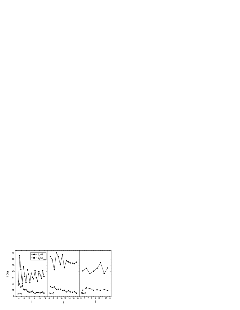
Figure 2: Fractions of states with ground state spins $J_{0}=0$ (circles connected by solid lines) and $J_{0}=J_{{\rm max}}$ (squares connected by dashed lines) for the single$-j$ models as a function of $j$. The three panels correspond to particle numbers $N=4,6$ and 8, from left to right, respectively. The uniform distribution of interaction parameters $V_{L}\in[-1,1]$ was used.

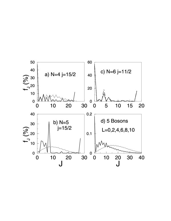
Figure 3: Distributions $f_{J}$ of ground state spins: $(a)$ 4 fermions on the $j=15/2$ level; $(b)$ 5 fermions on the $j=15/2$ level; in this odd-$N$ system, in accordance to panel $(a)$, the maximum of the probability corresponds to $J=j$; $(c)$ 6 fermions on the $j=11/2$ level; $(d)$ 5 bosons with interaction in the pair states with $L=0,2,4,6,8,10$, see Section 5. The uniform distribution of $V_{L}$ was used. The dotted lines in panels $(a),(b)$ and $(d)$ indicate the statistical distribution of multiplicities $d_{J}/d$; the dashed line in panel $(c)$ corresponds to the case with no pairing, $V_{0}=0$.

Various assumptions concerning the choice of ensemble lead to quite similar results for $f_{J}$ although details can differ. Along with this, it was observed [61, 66] that in many cases the fraction of the ground state spins equal to the largest possible— spin $J_{{\rm max}}$ is also considerably enhanced, see the last line of Table 1. Note that in the single-$j$ model (the results for $f_{0}$ and $f_{J_{{\rm max}}}$ in this case are shown in Fig. 2 as a fluctuating function of $j$) the state with $J=J_{{\rm max}}$ is unique being constructed by full alignment of the particles along the quantization axis (no random walk in this case). The effects persist for odd-$A$ [66], see also Fig. 3$b$, and odd-odd [68] nucleonic systems and for interacting bosons [61], see also Fig. 8. Typical examples are shown in Fig. 3. Structures of the wave functions, properties of the observables and excitation spectra also were studied in a multitude of models. We will discuss the most important findings as we go step by step testing the explanations put forward by various authors.

4.2 Induced pairing?

The first idea suggested for the explanation of the ground state spin effects [8, 59] was related to Cooper-type pairing induced by random interactions through some high-order mechanism. For a single $j$-level there are deep symmetry reasons to presume a special role of pairing since the seniority quantum number is only broken by about $1/3$ of $k=j+1/2$ linearly independent combinations of interaction parameters [57, 86]. The pairing idea was supported [8] by the enhanced gap between the ground and first excited states in the case of $J_{0}=0$, presence of odd-even staggering and the large pair transfer matrix element $\langle N-2|P|n\rangle$ between the ground states of adjacent even nuclei. The pair transfer operator $P$, however, was taken in such a form (different in different realizations) that in fact predetermined the result.

Table 1 contains important information about the role of explicit pairing (parameter $V_{0}$ in the Hamiltonian) in the single-$j$ case. Eliminating pairing completely from the dynamics, column $(i)$, does not noticeably change the fraction $f_{0}$. Even the transition to “antipairing” (fixed $V_{0}=+1$) only slightly reduces the value of $f_{0}$, column $(h)$. The attractive fixed pairing, $V_{0}=-1$, however, increases the fraction $f_{0}$ to 80%, column $(g)$. Similar results can be seen in Fig. 3$c$: in this case, $N=6$ and $j=11/2$, fully random interactions lead to $f_{0}=55.9$%, setting pairing to zero $V_{0}=0$ reduces fraction of $J_{0}=0$ ground states to $f_{0}=51.9$%, in “antipairing” case $f_{0}=44.4$% and finally, forced pairing with $V_{0}=-1$ leads to $f_{0}=82.7$%.

The fact that, as a rule, the ground state with $J_{0}=0$ does not contain considerable pairing correlations, can be seen from the observation based on the ICE, Section 2.4. Indeed, with forced pairing (by means of large negative $V_{0}$), many random realizations change the ground state structure undergoing a transition to the superconducting paired state. The ICE can be used here to study such transitions in each individual realization. In Fig. 4, left, the behavior of ICE for a few randomly selected realizations is shown as a function of the pairing strength $V_{0}$, around which the fluctuations necessary to obtain the ICE are imposed. All selected realizations had $J_{0}=0$ even without pairing, i.e. at $V_{0}=0.$ The peaks are observed in the ICE curves for all random realizations. The location of the peak roughly indicates the critical point of the phase transition with the maximum sensitivity to noise, while the sharpness of the peak and ICE magnitude reflect the size of the critical region. As one would expect, the properties of the pairing phase transition vary significantly from one sample to another. It is however clear that, in order for a significant fraction of random realizations to exhibit developed pairing, an average coherent attraction in the $V_{0}$ channel must be added, see right panel in Fig. 4, an analog of a displaced ensemble [80, 82].

Figure 4: On the left panel the invariant correlational entropy (ICE) for randomly selected realizations of ensemble is plotted as a function of pairing strength $V_{0}$. The system of six particles on $j=15/2$ level is chosen. Right panel shows the distribution of critical values $V_{0}$ defined as peaks on each ICE curve.

To find out if there is an important role of induced pairing, we compare directly the empirical ground state wave functions $|0\rangle$ with $J_{0}=0$ from the diagonalization in the random ensemble to the fully paired state $|s=0\rangle$ of seniority zero and the same particle number that can be built uniquely for a single-$j$ level. Fig. 5 shows with shaded histograms the distribution $P(x)$ of the overlaps

$$x=|\langle 0|s=0\rangle|^{2},\quad 0\leq x\leq 1,$$ (35)

for 4 and 6 fermions on the $j=15/2$ level, left and right panels, respectively, that have $d_{0}=3$ and $d_{0}=4$ states of $J=0$. The overlap (35) is one of the weights $w$ of the wave function, namely the one for the paired basis state. The paired structure would give a peak of $P(x)$ at $x\rightarrow 1$ while a random wave function is characterized by the distribution $P(x)$ of eq. (6). For $d=3$, left panel,

$$P_{d=3}(x)=\frac{1}{2\sqrt{x}},$$ (36)

with a peak at $x\rightarrow 0$ shown with solid line. This distribution appears in the problem of pion multiplicity from a disordered chiral condensate [87, 88], where isospin 1 determines the dimension $d=3$. Similarly, in the right panel, with a bigger space, $d_{0}=4$, the chaotic distribution is $P_{d=4}(x)\propto(1-x)^{3/2}x^{-1/2}$, and the empirical distribution displays only a slight excess near $x=1$, of the order of 1% in the total normalization.

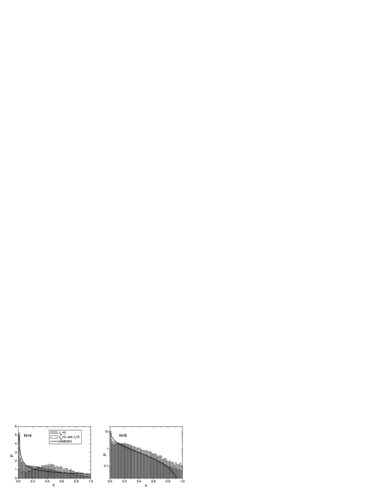
Figure 5: The distributions of overlaps $x$ between the ground states of spin zero in the random ensemble and states of seniority zero, for $N=4$, left, and $N=6$, right, fermions on the $j=15/2$ level, shaded histograms, for the ensemble of all random $V_{L}$. The solid lines show the statistical distributions expected for a chaotic system of dimensions $d=3$, left, and $d=4$, right. The unshaded distributions are calculated for the parts of the ensemble that give a ground state $J=0$ and the first excited state $J=2$.

A similar analysis with similar results was also carried out for the $sd$ shell model space [67], where the geometry is much richer and includes also isospin. The calculation of information entropy (3) revealed the chaotic character of eigenstates; even the ground state always has a high degree of complexity exceeding that for the realistic shell model. One can compare the ground state wave functions $|JT=00\rangle$ obtained with random interactions to those corresponding to the realistic system. With the standard effective interaction for this shell [89] (and the results were shown to change only slightly for different interactions), the comparison for ²⁴Mg ($N=8$ nucleons) provides the following average overlaps $x$ with the ground state wave functions for different random ensembles: (a) degenerate single-particle energies and all 63 two-body matrix elements generated as random uniformly distributed quantities: $f_{0}=0.591,\,x=0.020$; (b) realistic single-particle energies and random interaction matrix elements: $f_{0}=0.493,\,x=0.053$; (c) realistic single-particle energies and six pairing interaction matrix elements with $L=0$ and $t=1$, and random remaining 57 matrix elements: $f_{0}=0.678,\,x=0.106$; (d) single-particle energies and 57 non-pairing matrix elements set to zero, while the pairing matrix elements taken as random variables: $f_{0}=0.922,\,x=0.052$. In the cases of realistic single-particle levels and random interactions, the ensembles of two-body amplitudes were chosen in such a way that have a realistic ratio of their magnitude to the single-particle level spacings [67] in order to allow for fair comparison.

Although the large value of $f_{0}$ is common for all variants, we see again that the presence of regular pairing, case (c), increases the fraction $f_{0}$. The largest $f_{0}$ is observed in case (d), where the off-diagonal pair transfer amplitudes make quantum numbers $J=T=0$ preferable for an even number of pairs, whereas the competing influence of incoherent interactions and the mean field level splitting is absent. The average overlaps $x$ are small in confirmation of the conclusion carried over from the single-$j$ model that the ground state wave functions with random interactions are far away from realistic ones which are up to high extent determined by pairing, although presence of deformation in realistic nuclei is another factor reducing average $x$.

In systems with many double degenerate orbitals for spins $j=1/2$ [84], the fraction $f_{0}$ turns out to be close to 100%, which, at least partly, is, like in the previous case (d), induced by a great preponderance of off-diagonal pair transfers. Here one should mention that such a system reminds a quantum spin glass with random spin-spin interactions. In that case [90] the ground state spin increases $\propto\sqrt{N}$ as expected for random spin coupling. The crucial difference as compared to shell-model systems is in the type of random coupling. For quantum spin glasses the spin-spin interaction $({\bf s}_{1}\cdot{\bf s}_{2})$ is usually assumed. This is equivalent to a fixed relation 3:1 between the singlet and triplet parts of the interaction. Contrary to that, in shell-model systems those parts are fully uncorrelated.

One can notice that even in case (a) the average overlap of 2% is higher than what we would expect, eq. (2.6), from the uniform distribution of the components, $\sim 1/d\sim 0.3\%$ for the actual dimension $d=325$. The maximum effect of 11% is reached in case (c) due to the combination of two effects. First, the presence of realistic pairing lowers energies of states with paired particles. Second, the effective dimension $d^{\ast}$ is now smaller than $d$ because the contributions of non-paired states to the ground state are appreciably reduced. The stabilizing presence of the mean-field orbitals, case (b), also increases the overlap with the shell model ground state. To conclude, a small effect of induced pairing should be present but not as a main reason for the statistical predominance of $f_{0}$.

4.3 Time-reversal invariance?

The normal pairing ($Lt=01$ channel) is believed to be singled out as the most important part of residual nucleon-nucleon forces due to the maximum overlap of spatial wave functions of the paired particles [4]. The coherent effects of this residual attraction are enhanced by a greater density of states for such pairs since in this case any single-particle state $|1)$ is coupled to its time-reversed counterpart $|\tilde{1})$ that has, in the absence of external magnetic or Coriolis fields, exactly the same single-particle energy (Kramers degeneracy). The same reasoning is behind the assigning a special role to the Cooper pairs with zero total momentum and singlet spin state in superconductors.

Since the dynamical specificity of pairing forces converts the ground state into a condensate of time-reversed pairs, it is natural to invert the problem and hypothesize that the time-reversal invariance can imply the preponderance, at least in the statistical sense, of the ground states with $J_{0}=0$ [80]. This idea was checked by Bijker, Frank and Pittel [60] who explicitly included in the random two-body interaction a Hermitian but not $T$-invariant part assuming the interaction Hamiltonian in the form that was earlier studied as an example of the transition from the GOE to the GUE,

$$H=\cos\alpha\,H^{R}+i\sin\alpha\,H^{I},$$ (37)

where $H^{R}$ and $H^{I}$ are uncorrelated Gaussian variables with zero mean and the same variance of off-diagonal elements. Here, because of Hermiticity, the matrix elements of $H^{R}$ should be real and symmetric, and those of $H^{I}$ real antisymmetric (therefore no diagonal elements in $H^{I}$) with respect to the initial and final pair state of an interacting pair. Note that such a modification is impossible for the single-$j$ model and therefore is irrelevant for the explanation of the effect at least for this particular case.

As shown in Ref. [60], the violation of $T$-invariance in the form (37) slightly enhances the effect of predominance of $f_{0}$ rather than reduces it. This might be understood since the Gaussian ensemble with zero mean averages out all odd powers of $H^{I}$, eliminating whatever the direct result of its presence could be and leaving on average only a renormalization of the real part. Although eq. (37) keeps intact the total variance of the random Hamiltonian, the higher even moments are increased. Thus, if there was a trend (of different origin) of pushing a state with $J=0$ down, this trend would be amplified by the inclusion of $H^{I}$.

Nevertheless, the concept of $T$-invariance may be relevant for the problem we are interested in. Indeed, any state with $J\neq 0$ appears as a multiplet of degenerate states $|JM\rangle$ with various projections. For any given $M\neq 0$, the state $|JM\rangle$ violates the $T$-invariance by choosing the sense of precession of the angular momentum vector around the quantization axis. This is nothing but a spontaneous symmetry breaking when the symmetry of the ground state is lower than that of the Hamiltonian. As always in such situations, the symmetry is restored by the degeneracy with other states of the same multiplet. A physical branch of the excitation spectrum that restores the symmetry is rotation that change the orientation with no price in energy (Goldstone mode). In this sense the state with $J=0$ is indeed singled out.

4.4 Statistical widths?

Many authors, starting with Ref. [60], explored the idea that the statistical predominance of $J_{0}=0$ states is associated with the shape of the level density $\rho(E;J)$ for a given value of $J$. We have already mentioned that two-body interactions in a finite Hilbert space produce the level density close to Gaussian in each $J$-class around the centroid of all strength functions (13) $F_{k}(E)$ for the basis states $|k\rangle$ of this class. Then the spectrum has a centroid

$$\bar{E}_{J}=\frac{1}{d_{J}}{\rm Tr}_{J}H\equiv\langle H\rangle_{J},$$ (38)

and the statistical width

$$\sigma^{2}_{J}=\langle(H-\langle H\rangle_{J})^{2}\rangle_{J}.$$ (39)

The widths found as a result of statistical spectroscopy [18, 54] for a given realization, have to be averaged over the random ensemble.

It is natural to assume that the $J$-class with a larger statistical width has a greater chance to contain the ground state (that does not mean that the inverse statement is also correct). The results of Ref. [60] show that in the $sd$ shell model for 4 and 6 particles the statistical widths for $J=0$ are by approximately 10% larger than for $J=2$ and for other low values of $J$. Here one needs to notice that, even if this correlation of $\sigma_{J}$ and $f_{J}$ would be universally correct, we actually would simply reformulate the original question in another language, namely what is the reason for the greater statistical width of the $J=0$ class. But, moreover, the correlation is not sufficiently strong and not universal [70].

Figure 6: The average width $\sigma_{J}$ of the level distribution in the $J$ class as a function of $J$ for 6 particles in a single level $j=15/2$, solid line; predictions of the statistical formula, dashed line.

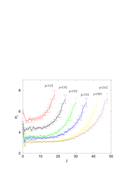
Figure 7: Widths $\sigma_{J}$ for various values of the level spin $j$ in the single-$j$ model as a function of $J$ for 6 particles.

Figs. 6 and 7 illustrate the situation with statistical widths in the single-$j$ models. Typically, $\sigma_{0}$ is greater than the widths of competing low values of $J$ but the widths $\sigma_{J}$ invariably grow higher than $\sigma_{0}$ for many large values of $J$. However, only the fraction of $J_{0}=J_{{\rm max}}$ is noticeably enhanced (still never on the level more than 15%) against multiplicity expectations. One can show that the difference in the widths has to be much greater, than it is in reality, in order to ensure, at comparable multiplicities $d_{J}$, the observed predominance of $J_{0}=0$ states. More subtle effects might be related [84] with deviations of higher moments of the statistical distribution from Gaussian ones, especially for a system of spins 1/2.

The comparisons based on pure statistical characteristics of individual $J$-classes are dangerous since they do not account for correlations between the classes which are at the core of the effect. If, for a given realization of the Hamiltonian, $g_{J}(E)=\rho(E;J)/d_{J}$ is the level density for the $J$-class normalized to unity, the probability of finding the levels of a given class at energy higher than $E$ can be written as

$$\chi_{J}(E)=\left(\int_{E}^{\infty}dE^{\prime}\,g_{J}(E^{\prime})\right)^{d_{J}}.$$ (40)

Then the probability of having the state $J$ below all other states will be

$$f_{J}=\int_{-\infty}^{\infty}dE\,\left[-\frac{d}{dE}\chi_{J}(E)\right]\prod_{J^{\prime}\neq J}\chi_{J^{\prime}}(E).$$ (41)

The densities of different classes in this formula are strongly correlated being determined by the same interaction. The task of averaging this many-point correlation function over the ensemble of random interactions is hardly solvable.

5 Mesoscopic effects of geometry

5.1 General idea

To find out how geometry of Hilbert space and of the random angular momentum coupling can induce the observed effects, we can first think of even simpler many-body problems [66, 71]. Take, for instance, a set of $N$ identically interacting spins,

$$H=\frac{1}{2}A\sum_{a\neq b}({\bf s}_{a}\cdot{\bf s}_{b}).$$ (42)

The energy spectrum of this system depends only on the total spin, ${\bf S}=\sum_{a}{\bf s}_{a}$,

$$E(S)=\frac{A}{2}[S(S+1)-Ns(s+1)],$$ (43)

where $s$ is the single-particle spin. If in a random ensemble the interaction strength $A$ is symmetrically distributed with respect to zero we see immediately that the ground state spin will be either $0$ (antiferromagnetic ordering, $A>0$) or the maximum spin $S=Ns$ (ferromagnetic ordering, $A<0$), both values appearing with probability $f_{0}=f_{{\rm max}}=1/2$.

In this primitive example the answer is simple because the spectrum of the system is pure rotational and all other quantum numbers, except for the exact constant of motion, $S$, are not differentiated by the interaction. We can expect that in all cases, when the coupling of individual spins plays a role, rotational modes (as we discussed above, they are Goldstone excitations restoring the orientational invariance) with the most ordered spin coupling schemes will bring in an enhanced probability for the lowest and the highest value of the ground state spin. The resulting probabilities are decided by the statistical weights of regions in the parameter space with positive and negative signs of the moment of inertia. The similar situation takes place in the case of pairing that is in fact rotation in gauge space: the energy of a state of seniority $s$ (a number of unpaired fermions) in the degenerate model for $N$ particles is [2]

$$E(s)=\frac{G}{4}(N-s)(2\Omega-s-N+2),$$ (44)

where $\Omega$ is the space capacity. Again, the ground state is either fully paired one, $s=0$, or “antipaired” one, $s=N$, depending on the sign of the pairing constant $G$. Instead of the rotation operator one has here quasispin that is the generator of $SU(2)$ algebra made of the pair transfer operators $P,P^{\dagger}$ and particle number operator $N$.

The situation is very similar in the case of isovector pairing on a single level. Here the problem can also be solved exactly with the use of $R(5)$ group formed by six isovector pair creation and annihilation operators, three components of isospin vector and total particle number [91, 92, 93]. The Hamiltonian

$$H_{{\rm i.p.}}=V_{0\,1}\,\sum_{\tau=0,\pm 1}P^{\dagger}_{\tau}\,P_{\tau}\,,$$ (45)

has energy eigenvalues

$$E=\frac{V_{0\,1}}{\Omega}\left[\frac{1}{4}(N-s)(2\Omega-N-s+6)+t(t+1)-T(T+1)\right]\,,$$ (46)

here as before $s$ is a number of unpaired nucleons while $t$ denotes their total isospin. The presence of the exactly conserved $SU(2)$ subgroup of isospin makes this example particularly interesting. The correlations between states with different isospin are represented by the term $T(T+1)$ which indicates the presence of rotational $V_{0\,1}<0$ or antirotational $V_{0\,1}>0$ bands with 50-50% probability. In quadrupole boson models a similar situation occurs often [61] with the presence of two “rotational” Casimir operators, three-dimensional, $\propto J(J+1)$, and five-dimensional, $\propto v(v+3)$, where the boson seniority $v$ characterizes the $O(5)$ group.

In a general case of complicated fermion dynamics, we can expect that the geometric chaoticity will on average single out global rotational modes, so that one can speak about an average Hamiltonian that describes the relative positions of the classes of states with different exact quantum numbers, such as total spin and isospin. The same logic works in the case of a similar problem of the ground state spin in chaotic quantum dots [94]. In our case the effective Hamiltonian $\tilde{H}$ of classes will take the form of the expansion in powers of the scalar constant of motion ${\bf J}^{2}$,

$$\tilde{H}=H_{0}+H_{2}{\bf J}^{2}+H_{4}({\bf J}^{2})^{2}+\,...$$ (47)

The coefficients in this expansion are functions of the random parameters in the original Hamiltonian. In the presence of additional conserved quantities, as isospin, a similar expansion in powers of ${\bf T}^{2}$ is to be added to (47). The problem is in (approximate) calculation of the coefficients in this expansion and their averaging over random parameters. If, as happens in reality, the quadratic term $H_{2}$ dominates, it determines a rotational band with a random moment of inertia, and the situation is analogous to that in eq. (43). For $J_{{\rm max}}$, the expansion (47) may not work, and a special treatment may be needed. This program was first implemented in Refs. [66, 68, 71]. A very similar consideration independently and with different ideology was carried out for interacting bosons [61]; we first comment on the boson problem.

5.2 Boson correlations

Complicated fermion dynamics generate boson-like collective excitations. Various types of phonons, magnons and plasmons are just a few examples for macroscopic systems; shape vibrations and giant resonances are well studied in mesoscopic physics of nuclei and atomic clusters. Because only few branches of the spectrum of elementary excitations are collectivized, the bosonization of the many-fermion problem can lead to significant simplifications of the formalism and a more transparent physical picture. This is confirmed by many successes of the IBM [95], where the boson model is postulated including certain collective modes although their exact relation to the original fermion interaction is not rigorously derived. The regular methods of boson expansion of fermion operators were introduced in nuclear physics long ago, [96] for a single-$j$ level and [97] for a general level scheme, see the detailed review article [98]. The application of the boson picture to our problem seems promising, especially because numerous studies of the IBM with random interactions [61, 62, 63, 64, 65, 75] found a similar pattern of the predominance of $J=0$ ground states.

The IBM with two types of interacting bosons has [95] the parameter space sharply divided between the spheres of influence of different symmetries. For example, this can be illustrated by the peaks of the ICE [40] clearly marking the narrow transitional regions between the symmetries. Using an ansatz of the axially symmetric coherent intrinsic state generated by a mixture of bosons, $sp$ for the vibron model and $sd$ for a conventional nuclear IBM, as a trial function for the ground state [61], one can find the boundaries between the domains of different symmetry. The coherent state corresponds to the body-fixed frame with a certain orientation and undetermined spin; parity is also violated in the vibron intrinsic state. Then one needs to project out correct angular momentum states (it would be better but more complicated to minimize the trial energy after this projection) and find the energy spectrum in the space-fixed frame. A system of $p$-bosons is especially simple since here quantum numbers $N$ and $J$ determine the state uniquely (allowed total spins have the same parity as the boson number and each spin appears once). A similar geometrical pattern takes place with respect to isospin in odd-odd nuclei [68], where the same statistics is valid for quasideuteron pairs with $L=0,\,t=1$; as a result some empirical regularities emerge with random interactions.

As follows from Ref. [61], the different intrinsic shapes of the ground state, markedly separated in the space of trial parameters, correspond to different coupling schemes of angular momentum. Typically one gets, for an even boson number, the condensate of scalar bosons with the only value $J=0$ possible, condensate of deformed bosons with the rotational spectrum and the probability divided between $J_{0}=0$ and $J_{0}=J_{{\rm max}}$ according to the sign of the moment of inertia, and the condensate of multipole, dipole or quadrupole, quanta again with the same alternative. Taking into account the corresponding areas in the parameter space, one comes to a good agreement with “empirical” (numerical) data for the random ensemble. One can think of the used procedure as of a variational method of constructing the effective Hamiltonian $\tilde{H}$, eq. (47). In the $sd$ model $\tilde{H}$ includes, apart from the rotational term $H_{2}J(J+1)$, also an above mentioned term $H^{\prime}_{2}v(v+3)$. This picture does not account for the cases with $J_{0}$ or $v_{0}$ different from the edge values but the fraction of such cases is low. The IBM is however much simpler than fermion systems because the Bose-statistics creates condensates that in many cases regularize the angular momentum coupling.

Going to the fermion system, we can try to use the boson expansion method. The boson representation of pair operators should be a reasonable approximation at least for a dilute system [66, 63, 84] with particle number $N$ much smaller than the space capacity $\Omega$. It follows from the commutator (31) (for simplicity we use the single-$j$ model) that indeed under such conditions the pair operators $P$ and $P^{\dagger}$ have quasiboson properties:

$$[P_{L^{\prime}\Lambda^{\prime}},P^{\dagger}_{L\Lambda}]=\delta_{LL^{\prime}}\delta_{\Lambda\Lambda^{\prime}}+\;{\rm terms\;of\;order}\;\frac{N}{\Omega}.$$ (48)

Thus, we can introduce the ideal bosons $B_{L\Lambda}$ [$L$ even from 0 to $L=2j-1=\Omega-2$] and find the boson expansion in the (symbolically written) form

$$P_{L\Lambda}\approx B_{L\Lambda}+[B^{\dagger}BB]_{L\Lambda}+\,\dots.$$ (49)

In the crudest boson approximation, the boson image of the fermionic Hamiltonian is therefore the gas of $N_{B}=N/2$ noninteracting bosons with quantum numbers $L,\Lambda$ and energies equal to $V_{L}$,

$$H_{B}^{(0)}=\sum_{L({\rm even})}V_{L}B^{\dagger}_{L}B_{L}.$$ (50)

The ground state of $H_{B}^{(0)}$ is a condensate of all $N$ bosons in a mode with spin $L$ corresponding to the minimum $V_{L}$. With random choice of $V_{L}$, this leads to a preference for the ground state spin $J_{0}=0$ [66]. Indeed, assume that every $V_{L}$ has the same chance $1/k$ to be the smallest one. If the value of $L$, $L({\rm min})$, corresponding to the smallest $V_{L}$ equals zero, the total spin $J$ can be only zero as well, the case analogous to the $s$-condensate in the IBM. All other choices of $L({\rm min})$ create many degenerate states with energy $E=N_{B}V_{L({\rm min})}$ and various values of total $J$ allowed for a given number of bosons with $L=L({\rm min})$, including again $J=0$ on more or less equal footing. Summarizing all cases, we should obtain a $J_{0}=0$ preference. The degeneracy will be lifted by the interactions coming from higher boson expansion terms.

The situation is illustrated by Fig. 3d, where the distribution of ground state spins is shown, solid line, for an ensemble of 5 noninteracting bosons with random energies $V_{L}$ for $L=0,2,4,6,8$ and 10. The dotted line shows that the statistical distribution of multiplicities is similar to that in the Fermi-case. The predominance of $f_{0}$ is clearly seen being however lower here than for fermions. Since the fraction $\sim 1/k$ of the pure $s$-condensate falls off for larger systems, we conclude that the simple bosonic effect does exist but cannot explain the entire picture. A similar result is seen in Table 1 where the approximation of a 6-fermion system on a $j=21/2$ level with 3 bosons is shown in column $(b)$.

Figure 8: The distribution of ground state spins for bosons, $N=6,\,j=4$, left, and $N=7,\,j=6$ in the uniform ensemble of interaction parameters.

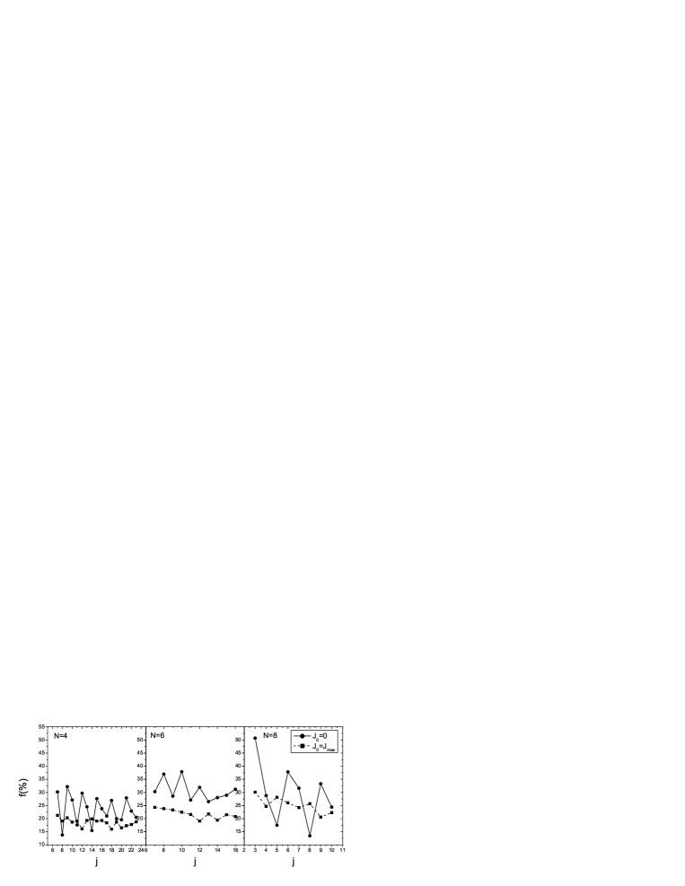
Figure 9: The systematics of probabilities $f_{0}$ for ground state spins $J_{0}=0$ (circles) and $J_{0}=J_{\rm max}$ (squares) in various systems of bosons; panels from left to right show $N=4,6$, and 8 cases as a function of integer single-boson spin $j$.

We can look also at the real interacting many-boson system constructed in analogy to our single-$j$ fermionic cases, Figs. 8 and 9. The situation here is similar to the IBM and shows that a considerable probability $f_{J}$ appears only for $J=0$, $J=J_{max}=Nj$, and $J=j$, which can be explained in the same way as in the IBM although the number of free parameters grows with $j$. Despite similarities, the overall boson statistics has some differences compared to the fermion case, see Figs. 2 and 9, in particular the probability $f_{0}$ is generally lower, averaging around 25-35 %. At the same time the probability of an “aligned” ground state with $J_{0}=J_{\rm max}$ is higher and for $N\ll 2j+1$ seem to stabilize at around 20-25%.

5.3 Sampling method and integrable systems

Table 1, column (f), shows the predictions for ground state spins in a system of $N=6,\,j=21/2$ obtained with the use of the practical recipe suggested by Zhao, Arima and Yoshinaga [74]. The results here are produced by the consecutive choice of the realizations of the random ensemble with only one nonzero parameter $V_{L}<0$. In these cases, the absolute value of this parameter is irrelevant. Thus, one performs the sampling of the “corners” of the parameter space. For each such extreme case, the diagonalization determines the ground state spin. The final prediction for the fraction $f_{J}$ comes as a fraction of the corners leading to $J_{0}=J$. Although this idea can be used for fast numerical estimates, it does not shed light on the physical reasons for the predominance of $J_{0}=0$ just adding another interesting observation.

The closest analysis of the recipe suggested in ref. [74] shows that the results of this procedure are nor always right, even qualitatively. A hard problem for such an empirical approach emerges for the ensembles with different weights for different matrix elements. The procedure does not indicate how the empirical fractions obtained for the corners are to be modified for such cases.

On the other hand, the corner evaluation indeed works in specific cases of integrable systems. Those are the cases when the eigenstates of the Hamiltonian can be labeled by exact quantum numbers as the consequence of rotational and some additional symmetries. It is known, for example, that for the single level $j=7/2$ all possible interactions preserve seniority, and the eigenstates are uniquely characterized by spin and seniority. Since the eigenfunctions do not depend on the interaction, the energy eigenvalues are linear functions of the interaction constants [73], and the coefficients of the linear form are still determined by geometry of angular momentum coupling. The search for the set of quantum numbers which provide the minimum of such a function is reduced to a problem of linear programming. An elegant geometric method of solving this problem was suggested by Chau et al. [85]. It is clear that the knowledge of corner energies is sufficient for this purpose.

The situation similar to that for fermions on $j=7/2$ orbit appears in systems of $p,d$ or $f$ bosons with interaction conserving the boson number. Again the appropriate quantum numbers are total spin and boson seniority. The analogous case was mentioned in the section on boson correlations for the systems that were not pure in boson composition (for example, $s$ and $p$ or $s$ and $d$ bosons) but were considered with the aid of the coherent variational function that introduced the condensate of a specific boson mixture. The result was more complicated because the proportions of mixture could depend on the interaction that would make the problem nonlinear. Almost in all cases one again sees the predominance of the states with extreme values of total spin or/and seniority.

6 Statistical approach

6.1 Effective Hamiltonian

In order to come to an estimate of average ground state energy for randomly interacting fermions we make a simple assumption that there is a mean field generated by the interactions in each realization of the ensemble and the field keeps axial symmetry so that one can speak about mean occupation numbers $n_{m}$ for fermions in an orbital with $j_{z}=m$ along the symmetry axis (again we limit ourselves by a formally simpler case of a single-$j$ level that still keeps the main features of the general problem). As discussed in Section 2.4, the interaction leads to equilibration so that the complicated states still can be characterized by the single-particle occupation numbers. We do not assume in advance thermal or other specific form of the equilibrium distribution; instead we can derive it from the simplest statistical arguments minimizing the ground state energy. In fact, we just assume that the ground state is as chaotic as excited states for the majority of realizations. This assumption is in line with what we had seen in the analysis of the overlaps of the actual ground state wave functions with fully paired functions and with the realistic shell model.

In the mean field approximation, the expectation value of the Hamiltonian (18) in a statistical state described by the occupation numbers $n_{m}$ can be written as

$$E(\{n_{m}\})=\frac{1}{2}\sum_{mm^{\prime}}V_{mm^{\prime}}\langle n_{m}n_{m^{\prime}}\rangle,$$ (51)

where the amplitudes $V_{mm^{\prime}}$ include the CGC,

$$V_{mm^{\prime}}=2\sum_{L\Lambda}V_{L}\left(C^{L\Lambda}_{jm\,jm^{\prime}}\right)^{2}.$$ (52)

Strictly speaking, eq. (51) contains the correlated occupation numbers taken for a given realizations and then averaged. In the simplest approximation we substitute this by the product $\langle n_{m}\rangle\langle n_{m^{\prime}}\rangle$ of mean occupation numbers; later the sign of averaging will be omitted.

The occupation numbers are subject to constraints due to the conservation laws of the particle number $N$ and total angular momentum projection $M$,

$$\sum_{m}n_{m}=N,\quad\sum_{m}mn_{m}=M.$$ (53)

Considering fully aligned states we identify the projection $M$ with total spin $J$. This is similar to what is routinely done in the nuclear cranking model when applied to the “rotation” around the symmetry axis, see for example [99]. In this case the angular momentum is explicitly built up by individual momenta of the constituents, in keeping with the main idea of geometrical chaoticity. Thus, we need to minimize the functional

$$\tilde{E}=\frac{1}{2}\sum_{mm^{\prime}}V_{mm^{\prime}}n_{m}n_{m^{\prime}}-\mu\sum_{m}n_{m}-\gamma\sum_{m}mn_{m},$$ (54)

where we added the constraints (53) with Lagrange multipliers of chemical potential, $\mu$, and cranking frequency (or magnetic field), $\gamma$.

The extremum of the functional $\tilde{E}(\{n_{m}\})$ is at the set $\{n_{m}\}$ that satisfies a system of linear algebraic equations

$$\sum_{m^{\prime}}V_{mm^{\prime}}n_{m^{\prime}}-\mu-\gamma m=0.$$ (55)

By solving for $n_{m}(\mu,\gamma)$ and applying the constraints (53), we find the appropriate values of the Lagrange multipliers $\mu(N,M)$ and $\gamma(N,M)$. The kernel (52) of this inhomogeneous equation contains random parameters and therefore in general can be inverted. The solution has a form of a linear polynomial in $m$ (constant occupation for $M=J=0$ and constant tilt for nonzero $J$). Finally, the value of energy for this solution is

$$E(N,M)=\tilde{E}(\{n_{m}(\mu(N,M),\gamma(N,M))\})+\mu(N,M)N+\gamma(N,M)M.$$ (56)

Moreover, since eq. (55) is still satisfied by this specific choice of $\mu$ and $\gamma$, it leads to

$$\sum_{mm^{\prime}}V_{mm^{\prime}}n_{m}(N,M)n_{m^{\prime}}(N,M)=\mu(N,M)N+\gamma(N,M)M,$$ (57)

that determines the energy at the extremum in the simple form

$$E(N,M)=\frac{1}{2}[\mu(N,M)N+\gamma(N,M)M]$$ (58)

that does not require an explicit expression for the occupation numbers. Of course, we just applied a standard procedure used in thermodynamics for the Legendre transformation between different potentials.

The value of the chemical potential can be found in a general way without actually solving the set of equations (55). Summing those equations for all $m$ and taking into account that

$$\sum_{m}1=2j+1\equiv\Omega,\quad\sum_{m}m={\rm Tr}\,j_{z}=0,$$ (59)

we obtain

$$\mu=\frac{1}{\Omega}\sum_{mm^{\prime}}V_{mm^{\prime}}n_{m^{\prime}}=\frac{2N}{\Omega^{2}}\sum_{L}(2L+1)V_{L},$$ (60)

where we used the normalization of the CGC,

$$\sum_{m\Lambda}\left(C^{L\Lambda}_{jm\,jm^{\prime}}\right)^{2}=\frac{2L+1}{\Omega}.$$ (61)

In a similar way we can calculate the cranking parameter $\gamma$. Multiplying eqs. (55) by $m$ and summing over $m$, we come to

$$\gamma=\frac{\sum_{mm^{\prime}}mV_{mm^{\prime}}n_{m^{\prime}}}{\sum_{m}m^{2}}=\sum_{L}V_{L}\sum_{m^{\prime}}n_{m^{\prime}}y_{L}(m^{\prime}),$$ (62)

where the geometric factor can be calculated as

$$y_{L}(m^{\prime})\equiv 2\sum_{m\Lambda}m\left(C^{L\Lambda}_{jm\,jm^{\prime}}\right)^{2}=\alpha_{L}m^{\prime},$$ (63)

$$\alpha_{L}=\frac{{\bf L}^{2}-2{\bf j}^{2}}{{\bf L}^{2}}\,\frac{\sum_{\Lambda}\Lambda^{2}}{\sum_{m}m^{2}}.$$ (64)

Since

$$\sum_{m}m^{2}=\Omega\,\frac{{\bf j}^{2}}{3},\quad\sum_{\Lambda}\Lambda^{2}=(2L+1)\,\frac{{\bf L}^{2}}{3},$$ (65)

the final result reads

$$\gamma=\frac{3}{\Omega^{2}{\bf j}^{4}}\sum_{L}(2L+1)({\bf L}^{2}-2{\bf j}^{2})\,M.$$ (66)

The geometric meaning of the combination in eq. (66) that determines the sign of the contribution of pairs with spin $L$ can be easily understood. By definition (6.4), for $M>0$, the energy (58) in the laboratory system goes to minimum for negative $\gamma$. The inequality ${\bf L}^{2}>2{\bf j}^{2}$ means that the constituents of the pair are aligned, and this contributes to the reduction of energy if there is attraction, $V_{L}<0$, for this component of the interaction. Vice versa, there should be repulsion, $V_{L}>0$, for antialigned pairs, ${\bf L}^{2}>2{\bf j}^{2}$.

Identifying $M$ with the magnitude $J$, we come to the effective Hamiltonian (47). In the statistical approximation, $\tilde{H}$ consists of only two terms, $H_{0}$ and $H_{2}$. The rotational term $H_{2}$ is in this approximation linear in random parameters. Therefore the crude prediction is that the probability of having the ground state spin $J_{0}=0$ is 1/2. Although the effective moment of inertia given by the inverse coefficient in front of $M$ in the parameter $\gamma$, eq. (66), does not depend on particle number, the statistical approach has to work better for a larger $N$. This is indeed seen in Fig. 2 where we juxtapose the results for $f_{J}$ in the systems of $N=4,6$ and 8.

One can also note [71] that the resulting prediction for the two items in energy, eq. (58), picks up the monopole, $K=0$, and dipole, $K=1$, terms in the Hamiltonian written in the multipole-multipole form (24) with an additional factor of two and the interaction parameters given by the transformation to the particle-hole channel (26); the $L$-dependence in the effective moment inertia (66) comes from the $6j$-symbol in eq. (3.17) for $\tilde{V}_{1}$. The extra factor of two originates from two possible recouplings of single particle operators in the two-body Hamiltonian on the way to the statistical approximation (51). The $K=0$ and $K=1$ multipole interactions are not independent from higher multipoles [eq. 28]. In the statistical limit the monopole term is produced in half by $\tilde{V}_{0}$ in eq. 24, while the other half comes from all higher $\tilde{V}_{K}$ combined via eq. 30, see also discussions and examples in [57].

The quality of the statistical description can be inferred from correlations of actual ground state energy in a given copy of the ensemble with the statistical value, Fig. 10. For the maximum possible momentum the statistical formula works nearly perfect, for the $J=0$ states the overall correlation is very good. However, exact energy is shifted down by a constant, which indicates correlations beyond the statistical description. This energy shift is shown in Fig. 11 as a function of the size of the space $j$ for a six particle system.

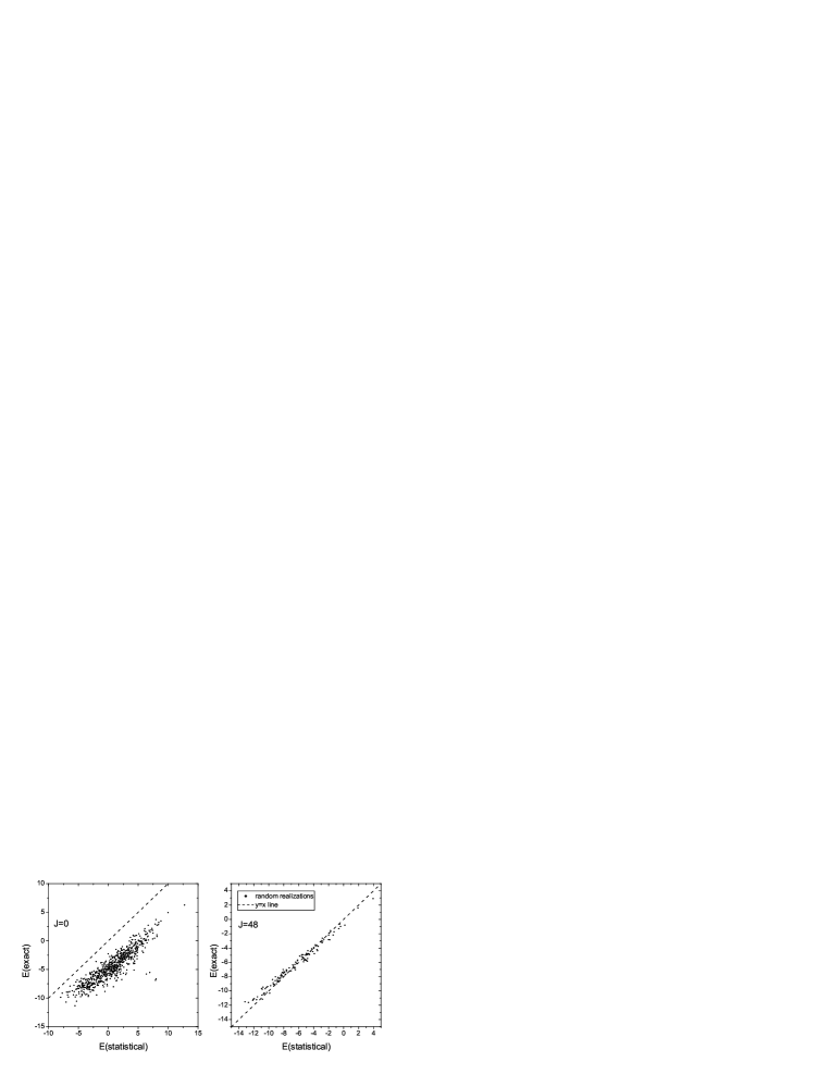
Figure 10: For a system of $N=6,\,j=21/2$, individual realizations with $J_{0}=0$, left panel, and $J_{0}=J_{{\rm Max}}$, right panel, are presented as points with coordinate $x$ equal to the value of energy from the statistical prediction and $y$-coordinate corresponding to the exact energy from diagonalization.

Figure 11: Average difference in energy between exact diagonalization and statistical prediction for systems of $6$ particles as a function of $j$.

6.2 Occupation numbers

The equivalence of the “monopole + dipole” truncation to the results of the lowest statistical approximation means that higher multipole interactions, being not associated with any conserved quantities, on average do not influence the equilibrium occupation numbers. This cannot be always true. Higher multipole interactions responsible for real deformation of the mean field lift the remaining degeneracies, compare the bosonic case. However, as $N$ and $\Omega$ grow, many competing multipoles tend to cancel each other. Therefore we expect the validity of the statistical approximation to improve as well. Essentially the same result can be derived by the direct calculation of the cranking model moment of inertia.

At the same time, the result above does not mean that the probability of $J_{0}=J_{{\rm max}}$ also goes to 50%. The multiplicity of the class with $J=J_{{\rm max}}$ is very low - in the single-$j$ model there exists only one such state with the unique full alignment of all available particles. Although this state by itself can be described well with the statistical approach, we cannot reliably compare the energy of this state with energies of states with other spins split due to the higher multipole interactions. The fact that the statistical description works for $J=J_{{\rm max}}$ is seen from Fig. 10 and Fig. 12, where the average values of the parameters, $\langle V_{L}\rangle$, obtained from the ensemble copies that resulted in $J_{0}=J_{{\rm max}}$, are compared to the statistical predictions.

Figure 12: Mean values $\langle V_{L}\rangle$ of interaction parameters for the cases with $J_{0}=J_{{\rm max}}$ in the $N=6,\,j=17/2$ system; numerical simulations, solid line, and statistical predictions, dashed line.

In Ref. [66] a stronger statistical assumption was made. The occupation numbers $n_{m}$ were modeled by those in a Fermi gas with high temperature when one can neglect dynamical splitting of single-particle orbitals $|jm)$, and the occupation numbers are determined solely by the constraints (53). In this case one can take

$$n_{m}=\frac{1}{1+\exp(-\alpha-\beta m)},$$ (67)

which ensures the statistical demands, $0\leq n_{m}\leq 1$, and includes, as in eq. (54), two parameters associated with the conservation laws (53). For any state with $J=M=0$, all orbitals $|jm)$ must have the same occupancy,

$$n_{m}=\langle 00|a^{\dagger}_{m}a_{m}|00\rangle=\frac{N}{\Omega}\equiv\bar{n}.$$ (68)

$\beta=0$, and the corresponding constant $\alpha_{0}$ is related to the particle number as

$$\alpha_{0}=\ln\,\frac{\bar{n}}{1-\bar{n}},$$ (69)

vanishing for the half-filled shell when $\bar{n}=1/2$. We usually try to avoid such systems which are exceptional, see for example [74], because of particle-hole symmetry that eliminates even-$K$ multipole moments.

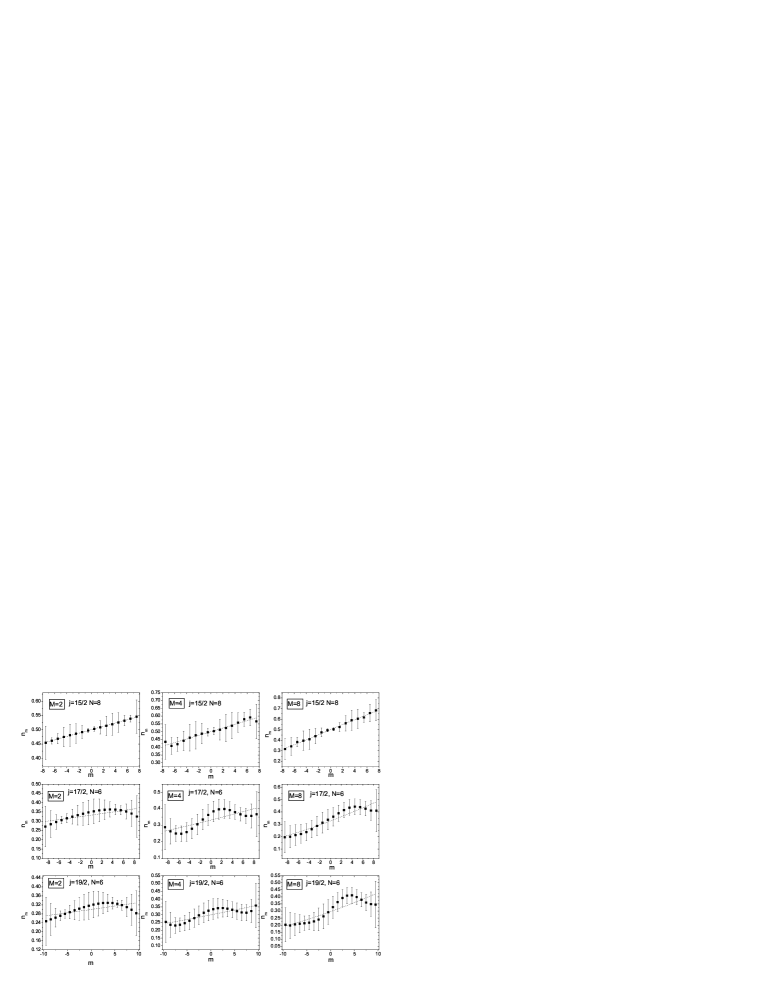
Figure 13: Average occupation numbers of yrast states of a given spin $J$ and projection $J_{z}=M=J$ for the $N=8,\,j=15/2$ system, top row; for $N=6,\,j=17/2$, middle row; and $N=6,\,j=19/2$, lowest row. Numerical results are shown with squares with error bars indicating rms deviations; statistical predictions are indicated with dotted lines.

For a nonzero total spin projection $M$, the parameter $\beta$, similar to the cranking frequency $\gamma$, creates a tilt of the function $n_{m}$. As shown in [66], the main effect is caught by the expansion of the distribution function (67) in powers of $\beta$. Due to time-reversal invariance, the parameter $\alpha$ acquires a correction in the second order, and the results are

$$\beta=\frac{M}{\bar{n}(1-\bar{n})}\sum m^{2},$$ (70)

$$\alpha=\alpha_{0}+\alpha_{2},\quad\alpha_{2}=\left(\bar{n}-\frac{1}{2}\right)\beta^{2}\frac{\sum m^{2}}{\Omega}.$$ (71)

In accordance with chaotic angular momentum coupling, a nonzero spin $M$ is created by the fluctuations of occupancies, $\propto\bar{n}(1-\bar{n})$, as in standard theory of level density of a Fermi-gas [49, 50]. The occupancies now can be written as

$$n_{m}=\bar{n}+\frac{mM}{\Omega\langle m^{2}\rangle}-\frac{\bar{n}-1/2}{\bar{n}(1-\bar{n})}\,\frac{M^{2}}{\Omega^{2}\langle m^{2}\rangle^{2}}\,(m^{2}-\langle m^{2}\rangle).$$ (72)

This approach works for bosons in the same way. In the case of $N$ bosons on a single $j$ level (integer $j$), the occupation numbers in the same approximation are given by

$$n_{m}=\frac{1}{\exp(-\alpha-\beta m)},$$ (73)

and the parameters can be found as

$$\alpha=\alpha_{0}+\alpha_{2},\quad\alpha_{0}=\ln\,\frac{\bar{n}}{\bar{n}+1},\quad\bar{n}=\frac{N}{\Omega},$$ (74)

$$\beta=\frac{M}{\bar{n}(1+\bar{n})}\sum m^{2},$$ (75)

$$\alpha_{2}=-\left(\bar{n}+\frac{1}{2}\right)\beta^{2}\frac{\sum m^{2}}{\Omega}.$$ (76)

The final result is analogous to (72):

$$n_{m}=\bar{n}+\frac{mM}{\Omega\langle m^{2}\rangle}+\frac{\bar{n}+1/2}{\bar{n}(1+\bar{n})}\,\frac{M^{2}}{\Omega^{2}\langle m^{2}\rangle^{2}}\,(m^{2}-\langle m^{2}\rangle),$$ (77)

which predicts the change of curvature compared to the Fermi expression (72). Note that the real condensate of bosons at a single $m$ value is impossible being in contradiction to the angular momentum requirement.

The expansion (72) is rapidly converging because of the powers of the “volume” $\Omega$ in the denominator. Using this for evaluating energies (51) of the states along the yrast line [66], one again comes to the effective Hamiltonian in the form (47), where the scalar and quadratic terms coincide with those found in the variational approach. The second order correction in (72) adds the quartic term $H_{4}\propto({\bf J}^{2})^{2}$. This contribution, which is small at not very high $J$, was taken in [66] to account for the difference between the observed fraction $f_{0}$ and its limiting statistical value of 1/2. Such corrections can be obtained with an improved variational ansatz of the previous subsection. As seen from Fig. 13, the actual occupation numbers for given $J=M$, averaged over the ensemble of yrast states with given $J$, indeed quite well follow the linear $m$-dependence. There are deviations from the simplest statistical and variational predictions. The last term in (72) includes kinematic correlations due to the Fermi-statistics, eq. 67, however it does not describe fully dynamical effects. The case of a half-occupied system is particularly interesting: here the fluctuations are significantly suppressed, see first row in Fig. 13; accordingly, the term proportional to $(m^{2}-\langle m^{2}\rangle)$ in eq. (72) disappears. However, a regular oscillatory behavior of the occupancies around the mean statistical behavior survives.

6.3 Multipole collectivity

We have seen earlier that the structure of the ground state is far from that of the paired condensate. The question if the set of random interactions generates, along with the ground states of zero spin, some collective structure of the excitation spectrum was put forward already in the original paper [8]. To find out the answer, the authors looked at the saturation of transitions from the ground state of $J_{0}=0$ to the first excited state of $J=2$ for a particle-hole operators of quadrupole type. They observed that it is possible to construct the quadrupole operator that maximally connects two states, and the resulting transition accumulates more than 50% of the corresponding sum rule, in similarity to the well known collectivity of the first $2^{+}$ states in non-magic even-even nuclei. In essence, this emphasizes a particle-hole nature of the transition with the operator adjusted to each copy of the random ensemble.

Actual quadrupole collectivity in nuclei is usually considered [100] as a result of coherent interactions in the particle-hole channel with $K=2$. The background created by pairing is important since the low-lying phonon collective excitation should be located within the energy gap due to pairing [5]. In a normal Fermi gas low-lying modes have nearly pure single-particle character. In contrast to that, in superfluid systems the presence of the gap stabilizes collective modes as coherent superpositions of two-quasiparticle excitations. At sufficiently strong collectivity, the mode found in the random phase approximation (RPA) becomes unstable, and then effects of anharmonicity lead to static deformation. In deformed nuclei, the low-lying quadrupole modes give rise to rotations and new vibrations around the deformed equilibrium point.

A comparison of “normal” quadrupole collectivity with data from the random interaction ensemble shows [67] that collective effects are strongly suppressed. One needs to ”displace” the ensemble including explicitly a coherent attractive part in order to reproduce the collectivity [80, 82], as was illustrated long ago by Cortes, Haq and Zuker [101]. The fractional collectivity suggested in Ref. [8] was calculated for 8 particles in the $sd$-shell model for ²⁴Mg using the realistic interaction [89] and various random ensembles mentioned above, Sect. 4.2. The degree of collectivity was defined as

$$f.c.=\frac{B({\rm E2};0_{1}\rightarrow 2_{1})}{\sum_{n}B({\rm E2};0_{1}\rightarrow 2_{n})},$$ (78)

where the reduced probability $B({\rm E2})$ of the quadrupole transition was determined with the fixed quadrupole operator rather than with different operators maximized for each set of random parameters. This quantity is significantly smaller than found in Ref. [8] for adjusted operators.

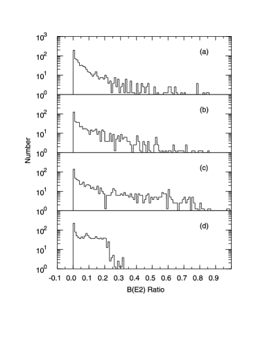
Figure 14: Distribution of probabilities $B({\rm E2};0_{1}\rightarrow 2_{1})$ in random ensembles $a-d$, Sect. 4.2, in units of the probability in realistic shell model for ²⁴Mg [89].

Fig. 14 shows calculated distributions of $B({\rm E2})$ for different ensembles (in units of the transition probability of 69.5 $e^{2}{\rm fm}^{4}$ found in the $sd$-shell model [89]) for ²⁴Mg. Typically, the $B({\rm E2})$ values from random interactions are by more than an order of magnitude weaker than in realistic calculations. Even the maximum $B({\rm E2})$ values out of 1000 samples for all four models are smaller than the realistic value, although is few copies they come close. The distribution of the $B({\rm E2})$ values for models (a) and (b) is close to the Porter-Thomas (6) as expected for matrix elements of a simple operator between two chaotic states [13, 28, 11]; the first excited state is even less regular than the ground state. The model (c) with realistic pairing generates a hint of collectivity. This agrees with what we have said above concerning the role of pairing correlations supporting the multipole collectivity. The sharp cutoff at small values of $B({\rm E2})$ in model (d) happens close to the value that can be obtained for the pure $(d_{5/2})_{p}^{4}(d_{5/2})_{n}^{4}$ configuration since here the multipole-multipole correlations generated by the higher-$L$ components of interaction are absent.

We have seen, Fig. 5, that, in spite of mainly chaotic nature of eigenstates for random interactions, there exists a slight excess of cases with a significant overlap between the ground state wave function and the fully paired state. This excess is particularly noticeable in cases when the sequence of the lowest states is $J_{0}=0,\,J_{1}=2$ (such cases appear also with a higher probability than could be expected from the statistical multiplicity). This means that there is a probability, exceeding the expectation of pure random models, that random interactions indeed create collective effects. To illustrate this point, we consider the dynamical quantity, which we call Alaga ratio, that can distinguish between different collective structures,

$$A=\frac{{Q}^{2}}{B(\rm E2)}.$$ (79)

Here the numerator is the expectation value squared of the quadrupole moment of the first excited state $2_{1}$,

$${Q}=\langle JM=J|{M}_{20}|J\,M=J\rangle\,$$ (80)

and the $B({\rm E2})$ transition strength in the denominator is defined as

$$B{\rm(E2)}=\sum_{M_{f}\kappa}\,|\langle JM_{f}|{M}_{2\kappa}|J\,M_{i}\rangle|^{2}\,.$$ (81)

Thus, limiting ourselves by the sequences $J_{0}=0,\,J_{1}=2$, we are looking at the ratio of diagonal to off-diagonal matrix elements of the quadrupole operator.

If random coupling of individual spins results in average spherical shape, and the ground and the first excited state are of similar structure, the Alaga ratio (79) should be small. On the other hand, if this random coupling creates a more or less rigid structure, one can expect the fulfillment of Alaga intensity rules [100],

$$A=\frac{4}{49}\equiv A_{0}\,.$$ (82)

For the two lowest states without any genetic interconnection, the Alaga ratio can take any value. In the case of single $j=15/2$ model, the sequences of interest appear in 6.7% for $N=4$ and in 9.2% cases for $N=6$. The distribution of the Alaga ratio for these systems, Fig. 15, reveals two peaks at $A=0$ and $A=A_{0}$. The peaks are pronounced stronger at a larger particle number. The idea that such structure can arise from random interactions is not that surprising. It was proven long ago [102] that the effects of interactions in large non-superfluid rotating Fermi-systems cancel leaving the rigid-body moment of inertia. In agreement with this, the statistical dependence of the level density, based on the geometrical chaoticity, also gives the same value of the moment of inertia, see [50] and eq. (12). The Alaga ratio seems to be a more sensitive signature of rotational behavior than the standard ratio of energies involving the next $J=4$ state.

Figure 15: The Alaga ratio for 6 and 4 particles in a single $j=15/2$ level; the histogram includes the states with the sequence $J_{0}=0,J_{1}=2$ of lowest spins.

6.4 Multipole dynamics

The multipole dynamics can be studied analytically starting with the operator equations of motion for the multipole operators $M_{K\kappa}$ and using the Hamiltonian in a suitable form (24) and commutation relations (33). The exact equations of motion are

$$[M_{K\kappa},H]=-g_{K}\sum_{K^{\prime}S}g_{K^{\prime}}g_{S}\tilde{V}_{K^{\prime}}[1-(-)^{K+K^{\prime}+S}]\left\{\begin{array}[]{ccc}K&K^{\prime}&S\\ j&j&j\end{array}\right\}$$

$$\times\sum_{\kappa^{\prime}\sigma}(-)^{\sigma}\left(\begin{array}[]{ccc}K&K^{\prime}&S\\ \kappa&\kappa^{\prime}&-\sigma\end{array}\right)\frac{1}{2}[M_{S\sigma},M^{\dagger}_{K^{\prime}\kappa^{\prime}}]_{+},$$ (83)

where $[...\,,\,...]_{+}$ denotes an anticommutator, and $g_{K}=\sqrt{2K+1}$. Note that zero values $K^{\prime}$ and $S$ do not contribute to these equations, and $K=0$ or 1 give trivial zero results because of the conservation laws.

We take in eqs. (83) the matrix element between the ground state $|0\rangle$, assumed to have zero spin, and a hypothetical collective state $|K\kappa\rangle$. After separating the dependence on magnetic quantum numbers by the Wigner-Eckart theorem,

$$\langle S\sigma|M_{K^{\prime}\kappa^{\prime}}|K\kappa\rangle=(-)^{\sigma+\kappa^{\prime}}\left(\begin{array}[]{ccc}S&K^{\prime}&K\\ -\sigma&-\kappa^{\prime}&\kappa\end{array}\right)M^{K^{\prime}}_{SK},$$ (84)

we come to the set of nonlinear equations for the matrix elements

$$M_{K}\equiv\langle 0|M_{K\kappa}|K\kappa\rangle\equiv(-)^{K}\frac{1}{g_{K}}\,M^{K}_{0K},$$ (85)

that contain the excitation energy $E_{K}$ of the collective state,

$$E_{K}g_{K}M_{K}=\sum_{K^{\prime}S}g_{K^{\prime}}g_{S}(\tilde{V}_{K^{\prime}}-\tilde{V}_{S})\frac{1-(-)^{K+K^{\prime}+S}}{2}\left\{\begin{array}[]{ccc}K&K^{\prime}&S\\ j&j&j\end{array}\right\}M_{K^{\prime}}M^{S}_{K^{\prime}K}.$$ (86)

Those equations are still exact if the sum runs over all allowed intermediate states of spin $K^{\prime}$.

In the spirit of the RPA we make here truncation leaving only the most coherent contributions with $K^{\prime}=K$ when the multipole $K$ does not share its angular momentum with other excitations. Thereby the equation gets linearized, and we obtain a closed expression for the excitation energy

$$E_{K}=\sum_{S({\rm odd})}g_{S}(\tilde{V}_{K}-\tilde{V}_{S})\left\{\begin{array}[]{ccc}K&K&S\\ j&j&j\end{array}\right\}M^{S}_{KK}.$$ (87)

The result (87) depends on expectation values $M^{S}_{KK}$ of odd-spin multipoles; the whole dynamics is concentrated in the differences $\tilde{V}_{K}-\tilde{V}_{S}$ of multipole coupling constants. The diagonal matrix elements of odd multipoles of rank $S$ can be constructed as those of irreducible tensors made of the $S$ components of angular momentum ${\bf J}$, another manifestation of fractional parentage or quasi-random geometrical coupling.

Using again the commutators (33) for odd $K^{\prime}$ and applying the same RPA-like approximation, we come to

$$M^{S}_{KK}=2g_{K}^{2}g_{S}\left\{\begin{array}[]{ccc}K&S&K\\ j&j&j\end{array}\right\},\quad S=\,{\rm odd}.$$ (88)

In the semiclassical limit of large $j$ the $6j$-symbol in eq. (88) is proportional to the Legendre polynomial $P_{S}(\cos\theta)$, where $\theta$ is the angle between ${\bf j}$ and ${\bf K}$. This describes the reorientation of the occupation numbers in the process of collective excitation by the multipole $K$. In this approximation, the collective excitation energy is given by

$$E_{K}=2g_{K}\sum_{S({\rm odd})}g_{S}^{2}(\tilde{V}_{K}-\tilde{V}_{S})\left\{\begin{array}[]{ccc}K&K&S\\ j&j&j\end{array}\right\}^{2}.$$ (89)

The earlier discussed statistical limit, $E_{K}\approx\tilde{V}_{1}K(K+1)$, is given by the contribution of the $S=1$ term. The other terms determine the collectivity corrections.

Figure 16: Transition energies between the ground state $J_{0}=0$ and the yrast state $J=K$ for a system $N=6\,j=15/2$ in a random ensemble compared to the RPA approximation, eq. (89).

Fig. 15 shows the correspondence between the excitation energies found in many runs with random interactions for the $N=6,\,j=15/2$ system and the RPA prediction (89). The strong correlation observed here confirms that, even for random interactions, the geometry of space and spin coupling forms coherent combinations that can be assessed with the regular methods of many-body theory. Also a horizontal line of point accumulation is seen that corresponds to the situation when the low-lying states are nearly degenerate. It would be interesting to study what part of the random parameter space corresponds to such absence of collective correlations.

7 Conclusion

The idea to study the physics of a finite mesoscopic system with random interactions turned out to be very fruitful. Many theoreticians responded to the challenge; many new things were learned even for the simplest systems of few identical particles; many questions are not answered yet. After four years of extensive studies the main result can be formulated as following: standard textbook ideas of the factors that form the low-lying structure of a closed self-sustaining mesoscopic systems are insufficient. The quantum numbers of the ground states and some regularities of spectra emerge not necessarily due to the corresponding coherent parts of the interparticle interaction. Up to a large extent, these characteristics are predetermined by the conservation laws and geometry of available single-particle space.

The angular moment $J_{0}=0$ of the ground state in even-even nuclei appears with a probability of the order 50% with any randomly taken rotationally invariant residual interaction. The underlying mechanism may be related to chaotic coupling of individual spins that creates an average yrast line described by the effective Hamiltonian with mainly quadratic dependence on total angular momentum. The time-reversible $J=0$ state turns out to have an exceptional ability of coming at the bottom or at the top end of the average spectrum. The strong attractive $L=0$ pairing of identical particles amplifies this effect and leads in reality to a 100% probability of $J_{0}=0$. Similar regularities are associated with odd-$A$ and odd-odd systems. We relied mostly on the nuclear structure as the basic and the best studied object of applications. However, the similar physics of random interactions and chaotic spin coupling certainly plays a role in other mesoscopic systems, such as atomic clusters, metallic grains, quantum dots and quantum spin glasses.

The new avenue were opened for general studies of quantum chaos. From extremes of random matrix theory based on the most general canonical Gaussian ensembles and later on the two-body random ensemble, we proceed to investigation of random interactions fully compatible with exact symmetries of finite systems. The new effects that enter the game now are correlations between the classes of states of different symmetry being governed by the common Hamiltonian with a relatively small number of random parameters. These correlations bring in the traces of new order and collectivity solely created by random interactions along with exact symmetries.

The pioneering paper [8] on the subject was concluded by the words that their studies “have barely scratched the surface of possible questions”. Now we know more and perhaps can say that we started to penetrate that surface. Nevertheless the problem is not entirely solved, and the future advances seem to be quite exciting and promising.

8 Acknowledgments

The authors are indebted to B.A. Brown, M. Horoi, D. Mulhall and J. Roebke for creative collaboration. Constructive discussions with G.F. Bertsch, R. Bijker, P. Cejnar, D. Dean, V.V. Flambaum, A, Frank, F.M. Izrailev, D. Kusnezov, T. Papenbrock, N.A. Smirnova, O.P. Sushkov, P. Van Isacker, H.A. Weidenmüller, Y.M. Zhao and A.P. Zuker at various stages of the work are gratefully acknowledged. We acknowledge support from the NSF, Grants Nos. PHY-0070911 and PHY-0244453, and from the US Department of Energy, Nuclear Physics Division, under Contract No. W-31-109-ENG-38.

References

- [1] G. Racah, Phys. Rev. 62 (1942) 438; 63 (1943) 367.
- [2] I. Talmi, Simple Models of Complex Nuclei (Harwood, New York, 1993).
- [3] M.G. Mayer and J.H.D. Jensen, Elementary Theory of Nuclear Shell Structure (Wiley, New York, 1955).
- [4] A. Bohr, B.R. Mottelson and D. Pines, Phys. Rev. 110 (1958) 936.
- [5] S.T. Belyaev, Mat. Fys. Medd. Dan. Vid. Selsk. 31 (1959) No. 11.
- [6] L.S. Kisslinger and R.A. Sorensen, Mat. Fys. Medd. Dan. Vid. Selsk. 32 (1960) No. 9.
- [7] B.A. Brown, Prog. Part. Nucl. Phys. 47 (2001) 517.
- [8] C.W. Johnson, G.F. Bertsch and D.J. Dean, Phys. Rev. Lett. 80 (1998) 2749.
- [9] V.V. Flambaum, A.A. Gribakina, G.F. Gribakin and M.G. Kozlov, Phys. Rev. A 50 (1994) 267.
- [10] V. Zelevinsky, B.A. Brown, N. Frazier and M. Horoi, Phys. Rep. 276 (1996) 85.
- [11] V. Zelevinsky, Annu. Rev. Nucl. Part. Sci. 46 (1996) 237.
- [12] Statistical Theories of Spectra: Fluctuations, ed. C.E. Porter (Academic Press, New York, 1965).
- [13] T.A. Brody, J. Flores, J.B. French, P.A. Mello, A. Pandey and S.S.M. Wong, Rev. Mod. Phys. 53 (1981) 385.
- [14] T. Guhr, A. Müller-Groeling, and H.A. Weidenmüller, Phys. Rep. 299 (1998) 189.
- [15] J.B. French and S.S.M. Wong, Phys. Lett. B 33 (1970) 449.
- [16] O. Bohigas and J. Flores, Phys. Lett. B 34 (1971) 261.
- [17] M.L. Mehta, Random Matrices (Academic Press, Boston, 1991).
- [18] V.K.B. Kota, Phys. Rep. 347 (2001) 223.
- [19] J.B. French, Rev. Mex. Fis. 22 (1973) 221.
- [20] K.K. Mon and J.B. French, Ann. Phys. (N.Y.) 95 (1975) 90.
- [21] V.G. Zelevinsky, Nucl. Phys. A555 (1993) 109.
- [22] F.M. Izrailev, Phys. Rep. 196 (1990) 299.
- [23] V. Zelevinsky, M. Horoi and B.A. Brown, Phys. Lett. B350 (1995) 141.
- [24] M. Horoi, V. Zelevinsky and B.A. Brown, Phys. Rev. Lett. 74 (1995) 5194.
- [25] I.C. Percival, J. Phys. B 6 (1973) L229.
- [26] J.J.M. Verbaarschot and P.J. Brussard, Phys. Lett. B87 (1979) 155.
- [27] G. Kilgus et al., Z. Phys. A326 (1987) 41.
- [28] O.P. Sushkov and V.V. Flambaum, JETP Lett. 32 (1980) 353; Sov. Phys. Usp. 25 (1982) 1.
- [29] N. Auerbach and B.A. Brown, Phys. Lett. B340 (1994) 6.
- [30] V.P. Alfimenkov et al., Nucl. Phys. A398 (1983) 93.
- [31] J.D. Bowman et al., Phys. Rev. Lett. 65 (1990) 1192; C.M. Frankle et al., Phys. Rev. Lett. 67 (1991) 564.
- [32] G.E.Mitchell, J.D.Bowman and H.A.Weidenm ller, Rev. Mod. Phys. 71 (1999) 445.
- [33] G.V. Danilyan et al., JETP Lett. 26 (1977) 186.
- [34] G.A. Petrov, Nucl. Phys. A502 (1989) 297.
- [35] V. Zelevinsky and A. Volya, Yad. Fiz. 66 (2003) 1829 [Phys. At. Nucl. 66 (2003) 1781].
- [36] V.V. Flambaum, F.M. Izrailev and G. Casati, Phys. Rev. E 54 (1996) 2136.
- [37] V.V. Flambaum and F.M. Izrailev, Phys. Rev. E 55, (1997) R13; E 56 (1997) 5144.
- [38] M. Srednicki, Phys. Rev. E 50 (1994) 888.
- [39] V.V. Sokolov, B.A. Brown and V. Zelevinsky, Phys. Rev. E 58 (1998) 56.
- [40] P. Cejnar, V. Zelevinsky and V.V. Sokolov, Phys. Rev. E 63 (2001) 036127.
- [41] A. Volya and V. Zelevinsky, Phys. Lett. B, in press (2003).
- [42] A. Peres, Quantum theory: Concepts and Methods (Kluwer, Dordrecht, 1995).
- [43] M.A. Nielsen and I.L. Chuang, Quantum Computation ands Quantum Information (Cambridge University Press, 2000).
- [44] T. Prosen and M. Z̆nidaric̆, J. Phys. A 35 (2002) 1455.
- [45] O. Bohigas, M.J. Giannoni and C. Schmit, Phys. Rev. Lett. 52 (1984) 1.
- [46] I.I. Gurevich and M.I. Pevzner, Nucl. Phys. 2 (1957) 575.
- [47] H.L. Harney, A. Richter and H.A. Weidenmüller, Rev. Mod. Phys. 58 (1986) 607.
- [48] T. Døssing et al., Phys. Rep. 268 (1996) 1.
- [49] H. Bethe, Phys. Rev. 50 (1936) 332.
- [50] T. Ericson, Adv. Phys. 9 (1960) 425.
- [51] E.P. Wigner, Am. J. Math. 63 (1941) 57.
- [52] G. Ponzano and T. Regge, in Spectroscopic and Group Theoretical Methods in Physics (North Holland, Amsterdam, 1968) p. 1.
- [53] L. Biedenharn and J.D. Louck, Angular Momentum in Quantum Physics (Addison-Wesley, Reading, 1981).
- [54] S.S.M. Wong, Nuclear Statistical Spectroscopy (Oxford University Press, New York, 1986).
- [55] N. Frazier, B.A. Brown and V. Zelevinsky, Phys. Rev. C 54 (1996) 1665.
- [56] A.L. Goodman, Phys. Rev. C 58 (1998) R3051.
- [57] A. Volya, Phys. Rev. C 65 (2002) 044311.
- [58] A. Volya, B.A. Brown and V. Zelevinsky, Phys. Lett. B 509 (2001) 37.
- [59] C.W. Johnson, G.F. Bertsch, D. J. Dean and I. Talmi, Phys. Rev. C 61 (1999) 014311.
- [60] R. Bijker, A. Frank, and S. Pittel. Phys. Rev. C 60 (1999) 021302.
- [61] R. Bijker and A. Frank, Phys. Rev. Lett. 84 (2000) 420; Phys. Rev. C 62 (2000) 014303; Phys. Rev. Lett. 87 (2001) 029201; Phys. Rev. C 64 (2001) 061303; Phys. Rev. C 65 (2002) 044316.
- [62] R. Bijker, nucl-th/0303069,
- [63] D. Kusnezov, N.V. Zamfir and R.F. Casten, Phys. Rev. Lett. 85 (2000) 1396.
- [64] D. Kusnezov, Phys. Rev. Lett. 85 (2000) 3773; 87 (2001) 029202.
- [65] L.F. Santos, D. Kusnezov and P. Jacquod, Phys. Lett. B 537 (2002) 62.
- [66] D. Mulhall, A. Volya and V. Zelevinsky. Phys. Rev. Lett. 85 (2000) 4016.
- [67] M. Horoi, B.A. Brown and V. Zelevinsky, Phys. Rev. Lett. 87 (2001) 062501.
- [68] M. Horoi, A. Volya and V. Zelevinsky, Phys. Rev. C 66 (2002) 024319.
- [69] D. Mulhall, A. Volya and V. Zelevinsky, Nucl. Phys. A 682 (2001) 229c.
- [70] V. Zelevinsky and A. Volya, in Challenges of Nuclear Structure, ed. A. Covello (World Scientific, Singapore, 2002) p. 261.
- [71] V. Zelevinsky, D. Mulhall and A. Volya, Phys. Atom. Nucl. 64 (2001) 525.
- [72] D. Mulhall, V. Zelevinsky and A. Volya, Acta Phys. Polonica B 32 (2001) 2491.
- [73] Y.M. Zhao and A. Arima, Phys. Rev. C 64 (2001) 041301.
- [74] Y.M. Zhao, A. Arima and N. Yoshinaga, Phys. Rev. C 66 (2002) 034302.
- [75] Y.M. Zhao, A. Arima and N. Yoshinaga, Phys. Rev. C 66 (2002) 064322, 064323.
- [76] A. Arima, N. Yoshinaga and Y.M. Zhao, Eur. Phys. J. A 13 (2002) 105,
- [77] N. Yoshinaga, A. Arima and Y.M. Zhao, J. Phys. A 35 (2002) 8575.
- [78] Y.M. Zhao, A. Arima and N. Yoshinaga, Phys. Rev. C 68 (2003) 014322.
- [79] S. Drozdz and M. Wojcik. Physika A 301 (2001) 291.
- [80] V. Velázquez and A.P. Zuker, Phys. Rev. Lett. 88 (2002) 072502.
- [81] Y.M. Zhao and A. Arima, nucl-th/0202056.
- [82] V. Velázquez, J.G. Hirsch, A. Frank and A.P. Zuker, Phys. Rev. C 67 (2003) 034311.
- [83] L. Kaplan and T. Papenbrock, Phys. Rev. Lett. 84 (2000) 4553.
- [84] L. Kaplan, T. Papenbrock and C.W. Johnson, Phys. Rev. C 63 (2001) 014307.
- [85] P. Chau Huu-Tai, A. Frank, N.A. Smirnova and P. Van Isacker, Phys. Rev. C 66 (2002) 061302.
- [86] G. Rosensteel and D. J. Rowe Phys. Rev. C 67 (2003) 014303.
- [87] A.A. Anselm, Phys. Lett. B 217 (1989) 169.
- [88] A. Volya, S. Pratt and V. Zelevinsky. Nucl. Phys. A671 (2000) 617.
- [89] B.A. Brown and B.H. Wildenthal, Annu. Rev. Nucl. Part. Sci. 38 (1988) 29.
- [90] J. Oitmaa and O.P. Sushkov, Phys. Rev. Lett. 87 (2001) 167206.
- [91] K. T. Hecht, Nucl. Phys. 63 (1965) 177.
- [92] K. T. Hecht, Phys. Rev. 139 B (1965) 794.
- [93] J. N. Ginocchio, Nucl. Phys. 74 (1965) 321.
- [94] J.A. Folk, C.M. Markus, R. Berkovits, I.L. Kurland, I.L. Aleiner and B.L. Altshuler, Phys. Scr. T90 (2001) 26.
- [95] F. Iachello and A. Arima, The Interacting Boson Model (Cambridge University Press, 1987).
- [96] S.T. Belyaev and V.G. Zelevinsky, Sov. Phys. JETP 15 (1962) 1004.
- [97] S.T. Belyaev and V.G. Zelevinsky, Nucl. Phys. 39 (1962) 582.
- [98] A. Klein and E.R. Marshalek, Rev. Mod. Phys. 63 (1991) 375.
- [99] A.L. Goodman, Phys. Rev. Lett. 73 (1994) 416, 1734.
- [100] A. Bohr and B. Mottelson, Nuclear Structure (Benjamin, N.Y., 1974) vol. 2.
- [101] A. Cortes, R.U. Haq and A.P. Zuker, Phys. Lett. 115B (1982) 1.
- [102] R.M. Rockmore, Phys. Rev. 124 (1961) 27.