Simulating the scalar glueball on the lattice

Abstract

Techniques for efficient computation of the scalar glueball mass on the lattice are described. Directions and physics goals of proposed future calculations will be outlined.

1 Introduction

Along with the mesons of the quark model, QCD allows for the existence of bound-states of gluons, the glueballs. The scalar glueball is the lightest state in the spectrum of strongly interacting gluons (described by the $SU(3)$ Yang-Mills theory) and in this consistent, confining quantum field theory, it is stable. The world of gluons alone thus provides an attractive starting point for investigations of glueballs. Confinement is not described at all within QCD perturbation theory and so computing properties of the glueballs requires a non-perturbative technique for studying strong interactions. As a result, no unambiguous identification of the scalar glueball has been made, although there is broad agreement that an extra state in the family of scalar resonances, unaccounted for by the quark model, exists between 1.5 and 1.8 GeV. In QCD, the glueball states will mix with the isoscalar resonances of the quark model, and will also decay strongly so to claim a complete understanding of the scalar mesons below 2 GeV therefore requires reliable knowledge of the masses and other properties of glueballs.

In order to disentangle the complex picture presented by experiments much more detailed and precise theoretical prediction from QCD must be made. At present, the only practical ab initio method for computing the non-perturbative properties of strongly interacting field theories such as QCD is through Monte Carlo simulation of the lattice regularisation of the theory. The glueballs of $SU(3)$ Yang-Mills theory have been studied extensively in lattice simulations Michael and Teper (1989); Bali et al. (1993); Morningstar and Peardon (1999), and this spectrum is becoming increasingly accurately determined. This is the first step in understanding the appearance of glueballs among the light scalar resonances of QCD. In spite of the limitation of these calculations, their output is proving to be very valuable in the construction and validation of phenomenological models.

In this article, we describe the state-of-the-art calculation of the glueball spectrum of the Yang-Mills theory. Investigations of further properties of these fascinating states, including their behaviour in QCD (with the dynamics of quark fields included) are then outlined.

2 Lattice QCD

Lattice QCD solves two key problems arising from strongly interacting gauge theories at a stroke; it provides both a non-perturbative regularisation of QCD and a means by which observables in the theory can be predicted by computer. This inherently gauge invariant regularisation is manifest through a direct cut-off of momenta at the Brillouin zone boundaries of the lattice.

To begin, the path-integral formulation of the theory in Euclidean space is taken. The four dimensions of space and time are discretised with a regular lattice of points separated by a spacing, $a$. In the gauge-invariant formulation defined by Wilson nearly 30 years ago Wilson (1974), the quark fields of QCD are defined at sites of the lattice, while the gluonic degrees of freedom are represented by parallel transporters (usually in the fundamental representation of the gauge group) connecting nearest-neighbouring sites. A definition of the Yang-Mills action is constructed from the trace of path-ordered products of the link variables around small loops on the lattice. The smallest non-trivial loop on the lattice circumnavigates a square of side-length $a$, usually called a plaquette. Similarly, a number of different definitions of the quark bilinear action, coupled to the gluons, can be made.

Path integral expectation values can then be estimated by numerical methods. If the theory is considered for space and time inside a finite-sized box, the path integral at non-zero lattice spacing is reduced to a very-high-dimensional ordinary integral. This type of problem can normally only be addressed by Monte Carlo methods, where a stochastic sampling of points inside the phase space to be integrated over is made.

2.1 Stochastic estimation methods for quantum field theory

After Wick rotation, the path integral for field theories such as QCD (at least at zero chemical potential) can be regarded as a statistical mechanical partition function. The Boltzmann weight for a particular field configuration is real and positive definite, and so can be interpreted as a statistical probability of the configuration appearing. In these circumstances, the natural Monte Carlo method to employ is importance sampling. An update algorithm is defined which generates configurations of the gluon fields, $U$ with probability density given by the Boltzmann weight, $\exp\{-S(U)\}$. The method is employed on the computer to generate an ensemble of gluon field configurations. Expectation values are then estimated from ensemble averages.

To compute the physical properties of the theory appropriate observation functions on the underlying fields are defined with the required quantum numbers, and these observables are measured on all members of the stochastic ensemble. Careful analysis allows a reliable determination of statistical uncertainties.

2.2 Controlling simulation artefacts

In order to make contact with the continuum field theory, a number of artefacts of the method must be controlled. The most obvious of these is the need to use a finite-sized box for numerical work. In practical simulations, boxes with side lengths of the order of 2 fm are feasible.

In many cases, the qualitative behaviour of states in increasingly large-but-finite volumes can be predicted. Simulations are run for a range of box sizes, and the data matched to this predicted form to allow safe extrapolation to the infinite volume limit. In most studies of glueballs these effects are now extremely small and do not constitute the dominant systematic error.

More difficult is the need to extrapolate data to the limit of zero lattice spacing (usually called the continuum limit). Again, the most natural procedure is to compute the physics of interest on a set of lattices with different grid spacings, and extrapolate. In many cases, the expected leading-order behaviour of these finite lattice spacing effects can be predicted, and this can be used to control data fitting. The problem with this direct approach is that the cost of computer simulations rises rapidly as the lattice spacing is diminished, at least in proportion to $a^{-4}$ and generally worse than this. Since the continuum limit exists at a critical point corresponding to a second order phase transition, where the correlation length of the system diverges in units of the lattice spacing, critical slowing down makes this cost higher. It is clear that the cheapest computer simulations are those run on the coarsest grids, which are furthest from the continuum.

2.3 Symanzik improvement

The effects of a finite grid spacing can be understood in the language of quantum field theory as arising from irrelevant operators appearing in the lattice action. These operators are of higher dimension than the relevant operator of the continuum theory, Tr $F_{\mu\nu}F_{\mu\nu}$ and are multiplied in the action by dimensionful couplings proportional to (positive) powers of the lattice spacing. For the simplest description of the gauge action, proposed by Wilson and consisting of the trace of the plaquette, the leading irrelevant operator appears at ${\cal O}(a^{2})$. Odd powers are prohibited by exact parity symmetry, which is preserved by the discretisation.

Universality suggests that there is a broad class of lattice representations of the continuum action, whose members all have the identical continuum limit: QCD. This implies that different lattice actions can be engineered which have smaller contributions from higher-dimensional operators. For asymptotically free theories, like QCD and the $SU(3)$ Yang-Mills theory of gluons, these discretisations of the action can be designed within the framework of perturbation theory. This concept is termed Symanzik improvement Symanzik (1983).

The idea has been widely exploited in lattice calculations, both in discretisations of gluon fields as well as the quark fields. For the gluon action, taking appropriate linear combinations of traces of larger closed loops, such as the $2\times 1$ rectangle means terms at ${\cal O}(a^{2})$ can be eliminated Luscher and Weisz (1985); Lepage (1996). This allows lattice investigations to be carried out with grid spacings as coarse as 0.25 fm, while remaining sufficiently close to the continuum limit to explore the physics reliably.

2.4 The anisotropic lattice

At the point in the calculation where measurements are made, these coarse lattices present new disadvantages. The mass of a state is extracted from the decay of a two-point correlation function in Euclidean space

$$C(t)=\langle\Phi(t)\Phi(0)\rangle\propto e^{-Mt}$$ (1)

where $\Phi(t)$ is a lattice operator that creates or annihiliates the state of mass $M$ at time $t$. This correlator falls exponentially as the two operators are moved further apart, and for a heavy state (such as the glueballs) the fall-off is rapid. Also, since the correlation function is being estimated in a Monte Carlo simulation, the statistical variance of the operators determines the accuracy to which these correlations can be measured. For the glueballs, these operators are the traces of closed Wilson loops on the underlying gauge fields and have rather large vacuum fluctuations, so a critical signal-to-noise problem arises. Since the operators can only be measured on points of the grid, little information can be extracted from coarse lattice measurements before the signal is lost in the noisy vacuum.

A solution that combines the economy of the coarse lattice with the good resolution of a fine grid is to use an anisotropic lattice, where the temporal lattice spacing is made small, while the three spatial dimensions are discretised more coarsely. Note that time-like correlation functions are used in extracting the masses of states. This method is particularly efficient for glueball simulations Morningstar and Peardon (1997). The two natural length scales in the problem, the mass and size of the glueball set the optimal temporal and spatial lattice spacings for numerical investigation.

Fig. 1 describes the output from just such an investigation. The figure shows the effective mass,

$$a_{t}M_{\rm eff}=\frac{\ln\;C(t)}{\ln\;C(t+1)}$$ (2)

for the scalar glueball measured on a highly anisotropic lattice, where the ratio of scales is $a_{s}/a_{t}=6$. The operator, $\Phi$ is constructed from a large basis set of the trace of closed Wilson loops built from smoothed link variables. A single operator for each state is made by taking linear combinations from the basis set of operators, with this combination chosen to optimise the overlap with the state of interest. The graph shows data for the ground-state scalar and the first excited state with the same quantum numbers. It illustrates the method is capable of precise determinations of the energies of both these levels. In the simulation presented in Fig. 1 these energies are measured to $1\%$ statistical precision.

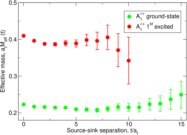
Figure 1: The effective mass plot of the scalar glueball channel, including data for the first excited state.

In Fig. 2, the dependence on the lattice cut-off of the scalar glueball mass in units of a physical scale $r_{0}$, derived from the static potential Sommer (1994), is presented. The data points represented with crosses are from a range of simulations performed using the Wilson plaquette action Michael and Teper (1989); Bali et al. (1993). The circles are from simulations with an anisotropic lattice action, improved according to the Symanzik programme with parameters determined from tree-level perturbation theory after the tadpole graphs in the lattice weak-coupling expansion have been resummed Morningstar and Peardon (1997, 1999). The quality of a lattice action should be judged by how strongly the mass (in physical units) depends on the cut-off; “better” actions should show a weaker dependence on the lattice spacing. By this assessment, the Symanzik improved action is superior to the simplest action, however a strong dependence on the cut-off still remains. The scalar glueball mass (in units of $r_{0}^{-1}$) falls as the lattice spacing is increased to reach a minimum from which it begins to rise again. We term this effect the “scalar dip.”

2.5 Curing the “scalar dip”

The lattice theory is not necessarily QCD; the physics of this theory is only recovered once the discretised version is “close” to the critical point on which QCD exists. If the space of lattice theories contains other critical points, simulations performed near to these points will be probing the properties of other continuum quantum field theories. Remarkably, this apparently abstract problem in non-perturbative renormalisation seems to arise in the simulation of $SU(3)$ Yang-Mills.

It has been recognised for some time that there is a line of “bulk” first-order phase transitions in the two-dimensional plane of lattice theories in which both a coupling to the fundamental and adjoint representations of the link variables is made Heller (1995). This line ends in a critical point at which some unknown continuum theory resides. If the physics of the lattice theory close to this critical point is investigated, it will be predominantly governed by the properties of this other theory. One suggestion is that the continuum theory at this critical point is a free scalar one, and if this was the case, the mass of the scalar particle in the lattice theory would be artificially light in comparison to the higher spin states. Precisely this artefact is observed.

The data represented by squares in Fig. 2 are from a new discretisation of the gluon action on an anisotropic lattice. In this prescription, the lattice action includes terms that trace over the link variables in the adjoint representation, as well as the fundamental. The links stored on the computer are in the fundamental representation, but the trace in the adjoint can be computed using the identity

$$\mbox{Tr }A(g)=\mbox{Tr }U(g)\;\mbox{Tr }U^{\dagger}(g)-1,$$ (3)

with $A(g)$ the adjoint representation of an element, $g\in SU(3)$ and $U(g)$ its corresponding fundamental representation.

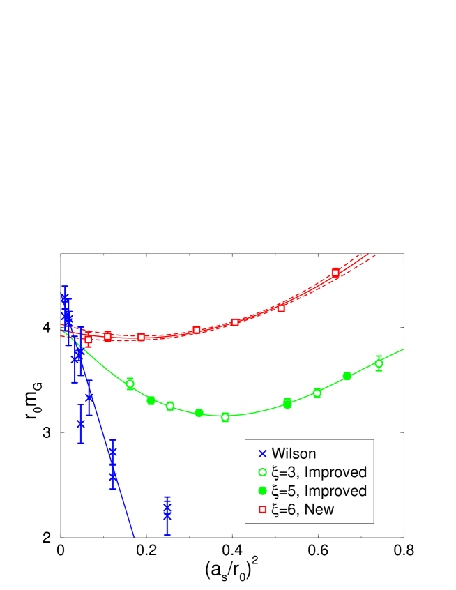
Figure 2: Extrapolating simulation data at finite lattice spacing to the continuum limit.

These simulation results are extremely encouraging and clearly show very weak lattice spacing dependence out to coarse spatial lattices ($a\approx 0.25$ fm). A very reliable extrabolation to the continuum limit can be made.

2.6 Spin on the lattice

In a scattering experiment, the spin of resonances is determined from a partial wave analysis. Revealing the spin of states in a lattice calculation requires similar care. Putting quarks and gluons onto a lattice breaks the continuum rotation group $SO(3)$ to the discrete cubic point group, $O_{h}$. As a result, states are no longer classified according to a spin quantum number which describes the irreducible representation (irrep) of $SO(3)$ they transform under. They have instead one of five labels corresponding to the five irreps of $O_{h}$: $A_{1},A_{2},E,T_{1}$ and $T_{2}$. Table 1 describes how the representation of $O_{h}$ subduced from spin irreps of $SO(3)$ subsequently decompose into irreps of $O_{h}$.

J	$A_{1}$	$A_{2}$	$E$	$T_{1}$	$T_{2}$
0	1
1				1
2			1		1
3		1		1	1
4	1		1	1	1

Table 1: The irreducible content of the representations of $O_{h}$ subduced from the spin irreps of $SO(3)$

To identify the spin of the state in the continuum, degeneracies across lattice states must be found and compared to the table. For example, tagging a spin 2 state on the lattice requires finding degenerate states in the $E$ and $T_{2}$ channels (and no others) in the continuum limit. For the scalar state, this procedure is quite straightforward; a state in the trivial representation, $A_{1}$, which is not degenerate with any other state in the spectrum can be uniquely identified with a continuum $J=0$ scalar. This spin analysis was carried out in Ref. Morningstar and Peardon (1999) for the glueball spectrum, and the spins of many continuum states were identified.

3 The $SU(3)$ Yang-Mills spectrum

Following the procedures outlined in the previous sections, the simulations of the Yang-Mills theory of strongly interacting gluons (without quarks) have reached high levels of precision. Fig. 3 shows the lightest six states in this spectrum of gluon bound-states. Note that both the ground-state and first-excited state in the scalar channel has been determined more reliably after removing the artefacts of the scalar dip and performing a continuum extrapolation. The masses of the scalar glueballs are consistent within errors with earlier determinations.

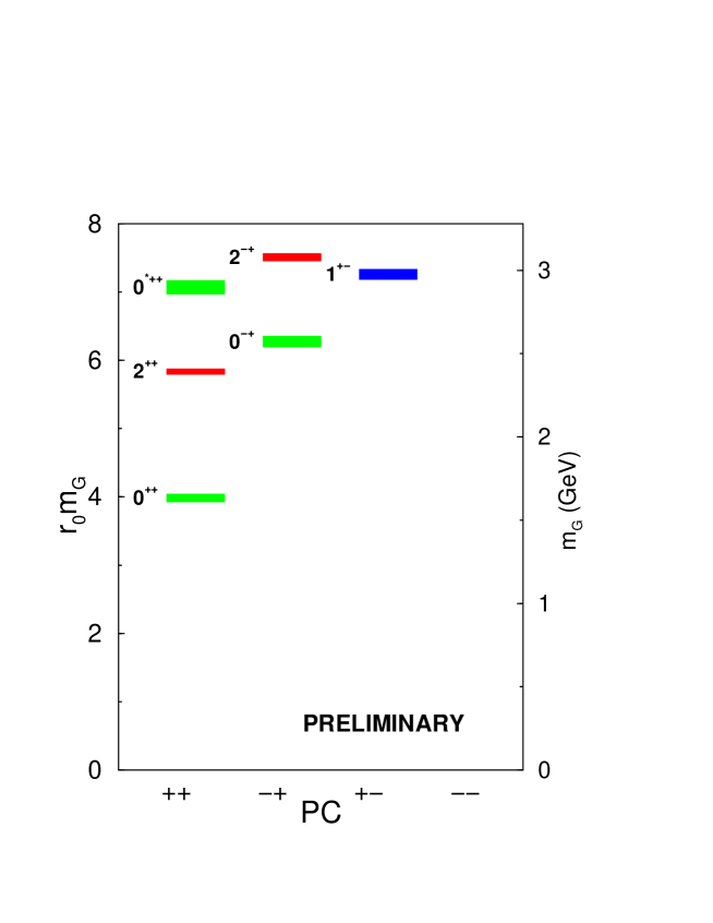
Figure 3: The lightest six states in the spectrum of the $SU(3)$ Yang-Mills theory.

4 Current and future directions

While the simulation of the Yang-Mills theory is now well understood, the inclusion of quantum fluctuations of quark fields is significantly more difficult. Since the Grassmann algebra of fermions in a path integral can not be handled directly by computers, the quark bilinear in the QCD action must be integrated out analytically, leaving a non-local effective action in the gluons alone. The non-local nature of these interactions means the simpler Monte Carlo algorithms used to generate ensembles of gauge field configurations for the Yang-Mills theories become inefficient. More sophisticated techniques are used, but they add a large numerical overhead; QCD simulations including quark dynamics are a factor of 100-1000 times more expensive than those of the Yang-Mills theory.

This issue of including the quark field dynamics remains a topic of a good deal of research in the lattice community and optimal simulation strategies are still actively under investigation. It seems likely that within the near future, the physics of glueballs that can decay into and mix with quark mesons will be investigated. Progress in this direction has begun by other lattice groups Hart et al. (2002) although lattice calculations involving unstable particles are in their infancy and remaind a challenging topic of research. Also, extending the anisotropic lattice technology, which proved so useful for scanning the pure gauge theory, to QCD simulations with dynamical quarks is under investigation.

5 Conclusions

Scalar mesons seem to constantly challenge theorists and phenomenologists by turn. At this meeting we heard of the difficulties in finding a convincing picture of the broad range experimental data and in this article, some of the quite distinct problems presented by the scalar glueball to lattice theorists have been outlined. Significant progress in this field is still being made and the Yang-Mills theory has now been mapped out. Full QCD dynamics, with the quark fields playing their role, is a major challenge under investigation by many members of the lattice community Lat03 . At the same time, more detailed properties of the gluonic theory are now being examined, including calculations of the chromoelectric and magnetic matrix elements Dong:Lat03 and the structure form factors.

References

- Michael and Teper (1989) Michael, C., and Teper, M., Nucl. Phys., B314, 347 (1989).
- Bali et al. (1993) Bali, G. S., et al., Phys. Lett., B309, 378–384 (1993).
- Morningstar and Peardon (1999) Morningstar, C. J., and Peardon, M. J., Phys. Rev., D60, 034509 (1999).
- Wilson (1974) Wilson, K. G., Phys. Rev., D10, 2445–2459 (1974).
- Symanzik (1983) Symanzik, K., Nucl. Phys., B226, 187 (1983).
- Luscher and Weisz (1985) Luscher, M., and Weisz, P., Phys. Lett., B158, 250 (1985).
- Lepage (1996) Lepage, G. P., Nucl. Phys. Proc. Suppl., 47, 3–16 (1996).
- Morningstar and Peardon (1997) Morningstar, C. J., and Peardon, M. J., Phys. Rev., D56, 4043–4061 (1997).
- Sommer (1994) Sommer, R., Nucl. Phys., B411, 839–854 (1994).
- Heller (1995) Heller, U. M., Phys. Lett., B362, 123–127 (1995).
- Hart et al. (2002) Hart, A., McNeile, C., and Michael, C., Nucl. Phys. Proc. Suppl., 119, 266–268 (2002).
- (12) See for example the proceedings of the XXI International Symposium on Lattice Field Theory (Lattice 2003), Tsukuba, Japan.
- (13) Chen, Y., et al., presentation by Dong, S-J. to the XXI International Symposium on Lattice Field Theory (Lattice 2003), Tsukuba, Japan.