Phenomenology of the $pp\to pp\eta$ reaction close to threshold

Abstract

The recent high statistics measurement of the $pp\to pp\eta$ reaction at an excess energy Q=15.5 MeV has been analysed by means of partial wave decomposition of the cross section. Guided by the dominance of the final state $\mbox{}^{1}S_{0}$ pp interaction (FSI), we keep only terms involving the FSI enhancement factor. The measured pp and $\eta$p effective mass spectra can be well reproduced by lifting the standard on-shell approximation in the enhancement factor and by allowing for a linear energy dependence in the leading $\mbox{}^{3}P_{0}\to\mbox{}^{1}S_{0},s$ partial wave amplitude. Higher partial waves seem to play only a marginal role.

I Introduction

In recent years major advances have been made in the experimental review ; meyer ; exp ; calen ; zupran ; moskal and theoretical eta_theo ; vadimm ; nakayama ; etap_theo ; kaiser investigation of the near threshold meson production reactions in nucleon-nucleon collisions (for a comprehensive review cf. review ). With the advent of medium-energy accelerators (ICUF, CELSIUS and COSY) and the corresponding influx of high precision data on the total and differential cross section as well as the polarization observables, it has become possible to study the interaction of the flavor-neutral mesons (eg. $\pi^{0},\,\eta$ and $\eta^{\prime}$) with nucleons. A direct insight into such interaction can not be gained from meson-nucleon scattering experiments as the latter are impractical owing to the very short life time of these mesons. Naturally, the largest data base has been accumulated for the pions meyer but the bulk of data on $\eta$ production in proton-proton collisions has also expanded significantly exp ; calen ; zupran ; moskal . The $\eta$ meson, which is the next lightest non-strange member of the pseudoscalar octet, has focused considerable attention of the nuclear community since it was established that the $\eta$-N interaction was quite strong and attractive which might lead to a possible existence of the $\eta$-nuclear bound states.

In the recent measurements of the $pp\to pp\eta$ reaction a very accurate determination of the four-momenta of both outgoing protons allowed for the full reconstruction of the kinematics of the final $\eta pp$ state. In consequence, these measurements provided in addition to the $\eta$ and the proton angular distributions, also the $pp$ and $\eta p$ effective mass distributions calen ; zupran ; moskal . The common feature of the near-threshold meson production in proton-proton collisions is the dominance of the very strong proton-proton final state interaction. The Monte Carlo simulations as well as direct calculations reveal that for small excess energies the inclusion of FSI enhances the cross section by more than an order of magnitude. This effect is also clearly visible in the effective mass distributions: as a prominent peak close to threshold in the pp effective mass distribution or as a bump near the end-point in the $\eta p$ effective mass distribution. The description in terms of a simple model in which a constant $\eta$ production amplitude is multiplied by an on-shell proton-proton FSI enhancement factor is only qualitatively correct, but at a quantitative level turns out to be insufficient to explain the experimental pp and $\eta$p effective mass distributions. The contribution from higher partial waves and the final state $\eta$p interaction have been indicated as the possible sources of this discrepancy. In comparison with pp interaction, however, the role of $\eta$-N interaction is much less important and taking as a rough measure the ratio of the $\eta$p and pp scattering lengths squared we may expect an effect at the level of about 1%. A full three-body calculation based on the hyperspherical harmonics method accounting for all pair-wise final state interactions corroborates the above estimate showing that the $\eta$p interaction modifies significantly only the total $\eta$ production cross section as function of the excitation energy whereas the distortion of the shapes of the effective mass distributions does not exceed the current experimental uncertainties. The hyperspherical harmonics method will be presented elsewhere HH and here instead we would like to confine our attention to a purely phenomenological description of the effective mass spectra at the lowest available excitation energy equal Q=15.5 MeV. At such a low Q only a few partial waves in both initial and final states are expected to participate in the $\eta$ creation process which substantially facilitates the interpretation of the experimental findings. Among the possible amplitudes the partial wave amplitude in which the two protons are deposited in the $\mbox{}^{1}S_{0}$ state plays a dominant role because it is proportional to the large FSI enhancement factor. Therefore, in the first approximation, in the cross section it should be sufficient to retain the square of the modulus of the dominant amplitude plus the interference terms that would contain the large FSI enhancement factor. However, after integrating over the angles the interference terms vanish and give no contribution to the pp effective mass distribution. This implies that there is really no room for improvements left unless a weak energy dependence is admitted in the dominant partial wave amplitude. We demonstrate in this paper that with this rather modest assumption both pp and $\eta$p effective mass distributions can be quite well reproduced.

The plan of our presentation is as follows. In the next Section the FSI enhancement factor is revisited. We argue that owing to a too steep a fall of the on-shell enhancement factor the approximate form thereof should be abandoned if favor of the full off-shell expression. Having established the best form of the enhancement factor we discuss the partial wave expansion of the $pp\to\eta pp$ transition amplitude in a quest of an approximate expression for the cross section that would be valid for the lowest excitation energies. Finally, in Section III we verify our simple model by presenting the comparison with experiment.

II Theoretical framework

II.1 Derivation of the enhancement factor

Since the proton-proton final-state interaction is believed to be the dominant ingredient in the description of the $pp\to pp\eta$ reaction close to threshold, it is logical that we first wish to reexamine the FSI problem to make sure that adequate measures have been taken to obtain the ultimate solution. The basic idea how to account for final state interaction was put forward 50 years ago by Fermi Fermi , Watson Watson , Migdal Migdal and others (for a review cf. Gold ; Omnes ; Giles ) and is based on the observation that in many processes the interaction responsible for carrying the system from the initial to the final state is of such a short range that in the first approximation may be regarded as point like. As a prototype one may consider a meson (x) production reaction $NN\to NNx$. To generate the meson mass m in nucleon-nucleon collision a large momentum transfer is required between the initial and the final nucleons, which is typically of the order $\sqrt{Mm}$, with $M$ being the nucleon mass. The corresponding ”range” of the production interaction is therefore much shorter than the range of the interaction between the two final state nucleons. Although it is perfectly true that the final state NN interaction significantly distorts the NN wave function but in the transition matrix element the contribution from all but the smallest NN separations will be strongly suppressed and the main effect may be attributed to the change of the normalization of the wave function at zero separation. If the non-interacting NN pair is described by a plane wave $\textstyle{\rm e}^{-\imath\,\bm{k}\cdot\bm{r}}$, where $\bm{k}$ is the relative NN momentum ($\hbar=c=1$ units are used hereafter), to account for final state interaction the latter must be replaced in the transition matrix element by the complete NN wave function $\Psi^{-}(\bm{k},\bm{r})^{\dagger}$ satisfying outgoing spherical wave boundary condition at infinity. Nevertheless, for a point-like interaction, we may set

$$\Psi^{-}(\bm{k},\bm{r})^{\dagger}\approx\textstyle{\rm e}^{-\imath\,\bm{k}\cdot\bm{r}}\;C(k)$$ (1)

in the matrix element so that the final state interaction will be accounted for by multiplying the transition matrix element by the enhancement factor, defined as

$$C(k)\equiv\displaystyle\lim_{r\to 0}\;\Psi^{+}(-\bm{k},\bm{r})/\textstyle{\rm e}^{-\imath\,\bm{k}\cdot\bm{r}}.$$ (2)

The factor $|C(k)|^{2}$ that appears in the cross section represents the ratio of two probabilities: one of finding the interacting NN pair at zero separation, while the other probability is associated with non-interacting particles. By construction, when the final state interaction is turned off, the enhancement factor will be equal to unity. Expanding both, the numerator and the denominator on the right hand side of (2) in partial waves, we have

$$C(k)=\displaystyle\lim_{r\to 0}\dfrac{\sum_{\ell=0}^{\infty}\;(2\ell+1)\,\imath^{-\ell}\,\psi_{\ell}(k,r)/r\;P_{\ell}(\hat{\bm{k}}\cdot\hat{\bm{r}})}{\sum_{\ell=0}^{\infty}\;(2\ell+1)\,\imath^{-\ell}\;j_{\ell}(kr)\,P_{\ell}(\hat{\bm{k}}\cdot\hat{\bm{r}})},$$ (3)

where $\psi_{\ell}(k,r)\sim r^{\ell+1}$ for small $r$, $j_{\ell}(kr)$ is spherical Bessel function and $P_{\ell}(\hat{\bm{k}}\cdot\hat{\bm{r}})$ denotes Legendre polynomial. Clearly, in the limit $r\to 0$ in (3), all higher partial waves will be suppressed by the centrifugal barrier, and only the contribution the from s-wave survives. Thus, we obtain a simple formula

$$C(k)=\psi_{0}(k,0)^{\prime}/k,$$ (4)

where prime denotes derivative with respect to $r$, and, as apparent from (4), the enhancement factor is determined by the slope of the wave function at the origin. To find this slope we must know the NN s-wave interaction and for simplicity we shall in the following assume that the latter takes the form of a spherically symmetric radial potential. The shape of this potential may be arbitrary but it must be of a short range. Given the NN potential, we can integrate outward the appropriate wave equation, containing both the nuclear and the Coulomb potential, generating numerically a regular solution $u_{0}(k,r)$ (i.e. vanishing at the origin) whose derivative satisfies the boundary condition

$$u_{0}(k,0)^{\prime}=C_{0}(\eta)\,k,$$ (5)

where $\eta$ denotes the Sommerfeld parameter and $C_{0}(\eta)^{2}=2\pi\eta/[\exp(2\pi\eta)-1]$ is the Coulomb barrier penetration factor. The sought for physical solution $\psi_{0}(k,r)$ occurring in (4) which is also regular, is necessarily proportional to $u_{0}(k,r)$, and, more explicitly, we have

$$\psi_{0}(k,r)=[C(k)/C_{0}(\eta)]\;u_{0}(k,r).$$ (6)

Now, all we need to calculate $C(k)$ is the asymptotic expression for the physical wave function. For $r=R$ with R much bigger than the range of the nuclear potential, the physical wave function takes the form

$$\begin{split}\psi_{0}(k,R)&=[C(k)/C_{0}(\eta)]\,u_{0}(k,R)=\\ &=F_{0}(\eta,kR)+f_{0}(k)\,H^{+}_{0}(\eta,kR),\\ \end{split}$$ (7)

where $H^{+}_{0}(\eta,kR)=G_{0}(\eta,kR)+\imath\,F_{0}(\eta,kR)$ with $G_{0}(\eta,kR)$ and $F_{0}(\eta,kR)$ being the standard Coulomb wave functions defined in Abram , and $f_{0}(k)=\sin\delta\,\textstyle{\rm e}^{\imath\delta}$ denotes the s-wave scattering amplitude with $\delta$ being the s-wave phase shift. The differentiation of (LABEL:C9) with respect to R, provides us with a second condition for the derivatives but it should be noted that $u_{0}(k,R)$ and $u(k,R)^{\prime}$ occurring in these two matching conditions are to be regarded as known quantities. Indeed, they are fully specified by the boundary condition at the origin (5) and can be either calculated analytically, or obtained by numerical methods. Therefore, what we end up with are two algebraic equations in which the two unknowns are the enhancement factor $C(k)$ and the scattering amplitude $f_{0}(k)$ and the respective solutions, can be conveniently written as

$$C(k)=\dfrac{k\,C_{0}(\eta)}{w[H^{+}_{0}(\eta,kR),u_{0}(k,R)]},$$ (8)

and

$$f_{0}(k)=-\dfrac{w[F_{0}(\eta,kR),u_{0}(k,R)]}{w[H^{+}_{0}(\eta,kR),u_{0}(k,R)]},$$ (9)

where the symbol $w[f,g]$ denotes the Wronskian defined as $w[f,g]\equiv fg^{\prime}-f^{\prime}g$. We wish to recall that the specific Wronskian involving the regular solution and the outgoing wave solution present in the denominator of (8) and (9) has been referred to as the Jost function Gold . It is worth noting that unlike the scattering amplitude (9) which can be expressed solely in terms of the logarithmic derivative of the regular solution, the enhancement factor (8) depends separately upon both, $u$ and $u^{\prime}$, and therefore the calculation of $C(k)$ requires off-shell information. In particular, a phase shift equivalent transformation of the potential may change the enhancement factor by orders of magnitude. Formula (8) may be cast to the form

$$C(k)=C_{WM}(k)\;\frac{(-k^{2})\,C_{0}(\eta)^{2}}{w[F_{0}(\eta,kR),u_{0}(k,R)]},$$ (10)

where

$$C_{WM}(k)=\frac{\textstyle{\rm e}^{\imath\delta}\sin{\delta}}{k\,C_{0}(\eta)},$$ (11)

is the familiar Watson-Migdal factor Gold , depending solely upon the on-shell quantities, whereas the Wronskian occurring in (10) represents the off-shell correction.

Formula (8) deserves some further comments. It is easy to check that when both, the Coulomb and the strong interaction are switched off, the enhancement factor (8) goes to unity. When the nuclear potential alone is set equal to zero, we have $u_{0}(k,R)=F_{0}(\eta,kR)$ and (8) yields $C(k)=C_{0}(\eta)$. Clearly, these are the right limits but they could not have been obtained with the Watson-Migdal factor alone which implies the importance of the off-shell correction. Nevertheless, close to threshold the off-shell factor varies slowly with energy, and the Watson-Migdal factor usually makes a good approximation. It should be kept in mind, however, that in result of multiplying the cross section by the Watson-Migdal factor the overall normalization is lost precluding an absolute calculation.

Some authors choose to simplify further the Watson-Migdal enhancement factor (11) by applying a Coulomb modified effective range formula for the phase shift. Thus, for the pp case, the phase shift can be obtained e.g. from the expression pp

$$\begin{split}C_{0}^{2}(\eta)\,k\,\cot{\delta}+2k\,\eta\,h(\eta)=&\\ =-1/a+b\,k^{2}/2&-P\,k^{4}/(1+Qk^{2}),\end{split}$$ (12)

with $h(\eta)={\text{R}e}\,\psi(1+\imath\,\eta)-\log(\eta)$ where $\psi$ is the logarithmic derivative of the gamma function. In (12) $a=-7.83~{}fm$ and $b=2.8~{}fm$ denote, respectively, the experimental pp scattering length and the effective range and the remaining two parameters ($P=0.73~{}fm^{3}$ and $Q=3.35~{}fm^{2}$) are related to a specific NN potential Nijm . The approximation (12) has been popular in ceratin quarters and used in conjunction with Watson-Migdal formula (11) for not very large k, results in a good approximation to the enhancement factor owing to a rather fortuitous cancellation of errors associated with different approximations.

II.2 Examples

We are going now to illustrate the results obtained in the preceding subsection by explicit calculations carried out for three phenomenological NN potentials which are: the delta-shell $V_{D}$, a Gaussian $V_{G}$, and the soft-core Reid $V_{R}$ potential Reid . Among these three potentials only Reid potential has a repulsive short-range component while the two remaining ones are purely attractive. The reason for selecting these particular shapes is that they exhibit different behavior in the close to the origin region: the delta-shell potential vanishes for small $r$, while a Gaussian potential shows maximum strength at $r=0$, and, finally, the Reid potential is singular at the origin, i.e. $V_{R}\to\infty$. Our purpose is to examine how this very different off-shell behavior influences the enhancement factor properties. Thus, as our first example we shall consider the delta-shell potential specified by a range $R$ and a dimensionless depth parameter $s$, defined by the formula

$$M\,V_{D}(r)=-(s/R)\,\delta(r-R),$$ (13)

where the values of the parameters are $R=1.84~{}fm$ and $s=0.906$. Although this potential is not realistic, its main advantage lies in its simplicity: both the phase shift and the enhancement factor may be for this case obtained in an analytic form. A simple calculation gives the phase shift

$$\tan\delta=\frac{(s/\rho)\,F_{0}(\eta,\rho)^{2}}{1-(s/\rho)\,F_{0}(\eta,\rho)\,G_{0}(\eta,\rho)}$$ (14)

where $\rho=kR$, and, respectively, the enhancement factor

$$C(k)=\frac{C_{0}(\eta)}{1-(s/\rho)\,F_{0}(\eta,\rho)\,H^{+}_{0}(\eta,\rho)}.$$ (15)

It is apparent from (15) that when the nuclear potential is switched off by setting $s$ equal to zero the enhancement factor reduces to the Coulomb factor $C_{0}(\eta)$.

The Gaussian potential $V_{G}(r)=V_{0}\,\exp{(-r^{2}/R^{2}})$ has also two parameters, the depth $V_{0}$ and the range $R$, whose values are $V_{0}=-31~{}MeV$ and $R=1.8~{}fm$ and in this case the the solution of the wave equation will be obtained numerically. Finally, we consider the fully realistic Reid soft core-potential Reid , given in the form of a superposition of three Yukawa potentials, which also requires numerical treatment.

The results of our computations are presented in Figs. 1 and 2.

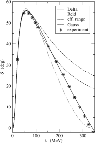
Figure 1: Momentum dependence of $\mbox{}^{1}S_{0}$ phase shift for different pp potentials.

In Fig. 1 we show the calculated pp phase shift vs c.m. momentum as obtained from the different potentials. They are compared with the data and we can see that up to about 150 MeV all models agree well with experiment. For bigger momenta the situation is less satisfactory, except for the Reid potential whose performance is still very good.

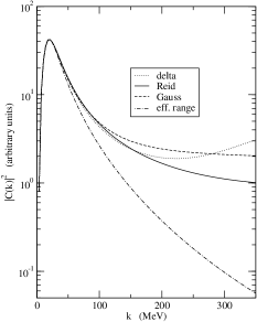
Figure 2: Enhancement factor $C(k)|^{2}$ vs. k for different pp potentials. The dot-dashed curve has been obtained form (11) and (12).

Clearly, among the considered potentials only the Reid potential has a repulsive core and therefore is capable of reproducing the crossover from positve to negative values in the phase shift at 340 MeV. In Fig. 2 we compare the enhancement factors calculated from formula (10) for different potentials. We stipulated the normalization as to get in all cases the same height at the maximum. It is evident from Fig. 2 that very good agreement between different potential models results sustains for momenta up to about 150 MeV indicating that, apart from normalization, different off-shell properties have little impact on the shape of the enhancement factor. This can be easily understood since close to threshold effective range approximation is usually adequate and all NN potentials are devised in such a way that they are capable of reproducing the experimentally determined effective range parameters. The main consequence of conducting a phase shift equivalent transformation is that the asymptotic wave function and its derivative acquire a common factor preserving thereby the shape of the enhancement factor. The differences appearing at larger momenta are not surprising as the different models do differ there also on-shell, as apparent from Fig. 1. In particular, as seen from Fig. 2, the effective range formula makes a reliable approximation for k not bigger than about 80 MeV. With the current high precision data, however, this approximation is insufficient causing a too rapid fall-off of the enhancement factor. Indeed, already for the excitation energy as low as Q=15.5 MeV and the maximal momentum $k_{max}=120~{}MeV$, $|C_{WM}(k_{max})|^{2}$ calculated from (12) is by a factor of 2 smaller from $|C(k_{max})|^{2}$ obtained from (10), with both functions normalized to yield the same height at the peak. In consequence, with the on-shell approximation the relative momentum distribution in the $pp\to pp\eta$ reaction has a too rapid fall off.

II.3 The cross section of the reaction $pp\to pp\eta$

Since close to threshold only a small number partial waves contribute to the $pp\to pp\eta$ transition amplitude, it is feasible to expand them in terms of angular momentum. The transition amplitude is an operator in spin space that depends upon the three c.m. momenta which determine the kinematics of the reaction, namely the initial proton momentum $\bm{p}$, the relative momentum of the final state protons $\bm{k}$, and, finally the momentum of the eta relative to the pp pair $\bm{q}$ (other possible choices will be discussed later on). The quantum numbers associated with the initial state are: the angular momentum $L$, the total spin $s_{i}$ and the total angular momentum J. In the final state, the angular momentum and the the total spin of the pp pair are denoted as $\ell$ and $s_{f}$, respectively, and the relative motion of the eta is described by the angular momentum $\lambda$. Among the above quantum numbers only J is conserved while the remaining quantum numbers are constrained by parity conservation and by the Pauli principle. Since the eta is a pseudoscalar meson, parity conservation requires that $L+\ell+\lambda$ must be an odd number. A list of possible transitions consistent with the above restrictions involving the lowest angular momenta is presented in Table 1.

Table 1: List of allowed transitions $\mbox{}^{2s_{i}+1}L_{J}\to\mbox{}^{2s_{f}+1}\ell_{J},\lambda$ for the lowest partial waves in the reaction $pp\to pp\eta$.

even $\ell$	odd $\ell$
$\mbox{}^{3}P_{0}\to\mbox{}^{1}S_{0}$,s	$\mbox{}^{1}S_{0}\to\mbox{}^{3}P_{0}$,s
$\mbox{}^{3}P_{2}\to\mbox{}^{1}S_{0}$,d	$\mbox{}^{1}D_{2}\to\mbox{}^{3}P_{2}$,s
$\mbox{}^{3}F_{2}\to\mbox{}^{1}S_{0}$,d	$\mbox{}^{3}P_{0}\to\mbox{}^{3}P_{1}$,p
$\mbox{}^{3}P_{2}\to\mbox{}^{1}D_{2}$,s	$\mbox{}^{3}P_{2}\to\mbox{}^{3}P_{2}$,p
$\mbox{}^{3}F_{2}\to\mbox{}^{1}D_{2}$,s	$\mbox{}^{3}F_{2}\to\mbox{}^{3}P_{1}$,p
	$\mbox{}^{3}F_{2}\to\mbox{}^{3}P_{2}$,p
	$\mbox{}^{3}P_{1}\to\mbox{}^{3}P_{0}$,p
	$\mbox{}^{3}P_{1}\to\mbox{}^{3}P_{1}$,p
	$\mbox{}^{3}P_{1}\to\mbox{}^{3}P_{2}$,p
	$\mbox{}^{3}F_{3}\to\mbox{}^{3}P_{2}$,p

These transitions can be classified as even or odd according to the value of the angular momentum $\ell$ of the final state protons. In the transition matrix element the even (odd) partial wave amplitude will be multiplied by an appropriate projection operator which is symmetric (antisymmetric) under the transformation $\bm{k}\to-\bm{k}$. Since the final state protons are indistinguishable all observables must be invariant under the interchange of the proton momenta, i.e. under the $\bm{k}\to-\bm{k}$ transformation. This means that all interference terms between even and odd states which are antisymmetric under $\bm{k}\to-\bm{k}$ transformation are bound to vanish if one wants to respect Pauli principle. In consequence, interference is allowed only between partial waves belonging to the same group which significantly reduces the number of terms in the cross section.

For small excitation energy the final state pp interaction appears to be the dominant effect and therefore it seems justified to neglect in the cross section all terms which do not contain the enhancement factor C(k). With this assumption the only contribution to the cross section comes from the even partial waves listed in Table 1. The partial wave amplitudes are functions of both, $k^{2}$ and $q^{2}$ but since these two quantities are linked by energy conservation one of them is redundant. Terms linear in k or q will be absent which can be seen as follows. The momentum dependence in a partial wave amplitude originates from the spherical Bessel functions $j_{\ell}(k\xi)\,j_{\lambda}(q\eta)$ occurring in the appropriate overlap integrals where $\xi$ and $\eta$ are the Jacobi coordinates canonically conjugated with k and q, respectively. For even orbital momentum the spherical Bessel function is an even function of the argument so that in the expansion of the partial wave amplitudes only even powers of the momenta will be admitted. However, for practical reasons, it does not seem feasible to go beyond the second order in k and q.

The above considerations lead us to take the following simple expression for the $pp\to pp\eta$ reaction cross section

$$\begin{split}\textstyle{\rm d}\sigma/\textstyle{\rm d}Lips&=|C(k)|^{2}\;[a+b\,P_{2}(\hat{\bm{p}}\cdot\hat{\bm{q}})]+\\ +&C_{0}(\eta)\;[d\;\text{Re}\,C(k)+e\;\text{Im}\,C(k)]\,P_{2}(\hat{\bm{p}}\cdot\hat{\bm{k}}).\\ \end{split}$$ (16)

In (LABEL:t1) we are using the standard notation where $\textstyle{\rm d}Lips$ stands for the invariant three-body phase space element. In (LABEL:t1) a denotes the modulus squared of the sole production amplitude which survives at threshold, associated with the transition $\mbox{}^{3}P_{0}\to\mbox{}^{1}S_{0},s$, b represents the interference term between the latter amplitude and the $\mbox{}^{3}P_{0}\to\mbox{}^{2}S_{0},d$ amplitude, and, the (d,e) pair describes, respectively, the interference with the $\mbox{}^{3}P_{2}\to\mbox{}^{1}D_{2},s$ amplitude. All of the above mentioned coefficients are functions of the final state momenta. Taking into account only threshold behavior, we can see that a is constant, b will be proportional to $q^{2}$ and (d,e) both are of the order of $k^{2}$. In this situation, we have to expand a to the same order setting $a=a_{0}+a_{1}\,q^{2}$ where $a_{0}$ and $a_{1}$ are two unknown parameters. The parameter $a_{0}$ can be absorbed in the normalization constant adjusted to the experimental total cross section value, and the ultimate expression for the cross section reads

$$\begin{split}\frac{\textstyle{\rm d}\sigma}{\textstyle{\rm d}Lips}&\propto|C(k)|^{2}\;\left\{1+\dfrac{q^{2}}{q_{max}^{2}}\,\left[x+y\,P_{2}(\hat{\bm{p}}\cdot\hat{\bm{q}})\right]\right\}+\\ +\dfrac{k^{2}}{k_{max}^{2}}&C_{0}(\eta)\;\left[z_{r}\;\text{Re}\,C(k)+z_{i}\;\text{Im}\,C(k)\right]\,P_{2}(\hat{\bm{p}}\cdot\hat{\bm{k}}),\\ \end{split}$$ (17)

where $x,y,z_{r},z_{i}$ are real dimensionless parameters to be determined. For reasons of convenience we have scaled q and k by dividing them by their maximal values $q_{max}$ and $k_{max}$, respectively. The parameter x represents the correction of the order $q^{2}$ to the dominant transition, the parameters y and $(z_{r},z_{i})$ provide the measure of the admixture of the d-waves.

III Comparison with experiment

In Fig. 3 and in Fig. 4 we present the experimental distribution moskal of the square of the effective pp mass $s_{pp}$ and the square of the $\eta$p mass $s_{\eta p}$, respectively. For a start, we assumed a constant production amplitude setting $x=y=z_{r}=z_{i}=0$. Using the on-shell enhancement factor $|C_{WM}(k)|^{2}$ specified in (11) with the effective range approximation (12), from (LABEL:t2) we obtain the theoretical distributions depicted by a dotted curve in Figs. 3 and 4.

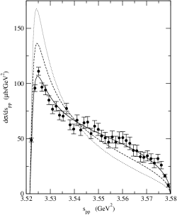
Figure 3: $s_{pp}$ distribution is compared with the data form Moskal et al. moskal . The dotted curve corresponds to a constant $\mbox{}^{3}P_{0}\to\mbox{}^{1}S_{0}\,s$ transition amplitude with on-shell enhancement factor (11) calculated from (12). In the dashed curve the complete $|C(k)|^{2}$ has been used while in the full curve, at the top of that, a correction linear in energy has been included.

Qualitatively, the dotted curves in Figs. 3 and 4 are roughly in accord with experiment but they are far not satisfactory in quantitative terms. In both figures the peak in the calculated curves is too big and partially responsible for that is the oversimplified enhancement factor. As we already know, $|C_{WM}(k)|^{2}$ calculated by using effective range formula (12) exhibits a too steep a fall and by normalizing the distributions to the total cross-section, to compensate that, the curves are moved up so that the peak gets magnified. Therefore, the simplest remedy is to abandon the on-shell approximation and from now on we will use the complete enhancement factor calculated from (10). The appropriate distributions are presented by the dashed curves in Figs. 3 and 4. Although the resulting corrections go in the right direction bringing the calculation closer to experiment, but this is still not enough for providing a full understanding of the data. In this situation, it is interesting to know how much we can improve the agreement by disposing of the various corrections discussed in the preceding section and represented by the adjustable parameters $x,\,y,\,z_{r},\,z_{i}$. Before proceeding, however, it should be observed that in the case of the pp effective mass distribution a major simplification takes place because, as apparent from (LABEL:t2), after integrating over the angles only the s-wave amplitude survives. Therefore, the parameters $y,\,z_{r},\,z_{i}$ representing interference terms never enter $s_{pp}$ distribution.

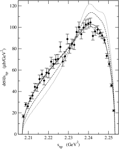
Figure 4: $s_{\eta p}$ distribution is compared with the data from Moskal et al. moskal . The dotted curve has been obtained keeping only the dominant $\mbox{}^{3}P_{0}\to\mbox{}^{1}S_{0}\,s$ transition amplitude which is assumed to be a constant with $|C_{WM}(k)|^{2}$ calculated from (12). In the dashed curve the complete $|C(k)|^{2}$ has been used while in the dot-dashed curve, at the top of that, a correction linear in energy has been included. The full curve accounts for also the interfernce with $\mbox{}^{3}P_{2}\to\mbox{}^{1}S_{0}\,d$ amplitude.

By contrast, in the case of $s_{\eta p}$ distribution the interference terms in general do not vanish in result of angular integration. Since a non-relativistic approach is here completely adequate, in order to obtain the cross section as a function of $s_{\eta p}$ we have to introduce an equivalent Jacobi frame taking as the two independent momenta the $\eta$-p relative momentum $\bm{k}_{1}$ and the momentum of the other proton relative to this pair $\bm{q}_{1}$. The transformation between the two Jacobi frames, takes the form

$$\binom{\bm{k}}{\bm{q}}=\begin{pmatrix}-1/2&-\mu/\nu\\ 1&-\mu/M\end{pmatrix}\binom{\bm{k}_{1}}{\bm{q}_{1}}$$ (18)

where $\mu$ is the eta-p reduced mass and $\nu$ is the reduced mass of the eta and the pp pair. Clearly, substituting (18) in (LABEL:t2) and integrating over the angles of $\bm{k}_{1}$ and $\bm{q}_{1}$, the interference terms give non-vanishing contribution.

Since the $s_{pp}$ distribution depends solely upon x, we adjusted this parameter by fitting the theoretical $s_{pp}$ distribution to the experimental data with the best fit value of x being x=-0.514. The resulting distribution displayed in Fig.3 by the full curve agrees now quite well with experiment. Actually, since the interference terms drop out and the $\eta$p interaction gives here a small effect, there is really not much room for improvement other than including the $q^{2}$ correction in the the dominant $\mbox{}^{3}P_{0}\to\mbox{}^{1}S_{0}\,s$ transition amplitude. Next, with the value of x in hand, we calculated the $s_{\eta p}$ distribution, still leaving out the interference terms i.e., setting $y=z_{r}=z_{i}=0$. The resulting cross section which does not involve adjustable parameters any more is presented in Fig.4 by a dot-dashed curve. We can see that also in this case the agreement with experiment looks much better. The interference terms in (LABEL:t2) involving the parameters $(z_{r},\,z_{i})$ are probably much smaller than the term proportional to y because the former terms exhibit only a linear dependence upon the enhancement factor, so we ignored these terms adjusting the single parameter y to the experimental $s_{\eta p}$ distribution. With x fixed, the best fit value of y was y=3.38. The corresponding cross section is displayed in Fig. 4 by the full curve and the agreement is quite good. We tried also to vary the parameters $(z_{r},\,z_{i})$ but this was not very successful as the fitting procedure attempts to reproduce a structure at the high energy end of the spectrum. With three adjustable parameters it is quite easy to produce a two-peaked distribution with a good $\chi^{2}$. Since it is not quite certain that the data really reveal a two-peaked distribution we did not pursue this fit any further. It should be also mentioned that when the interference term linear in C(k) is accounted for, the calculation becomes very sensitive to the NN potential used to obtain C(k) because the normalization of C(k) can not be absorbed in the overall normalization of the cross-section.

In Fig. 5 we are going to present the changes in the excitation energy distribution caused by adding an energy dependent term to the eta production amplitude (the interference terms in (LABEL:t2) give no contribution).

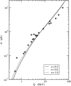
Figure 5: The total cross section for the $pp\to pp\eta$ reaction versus the excitation energy Q for different values of the parameter x. The experimental data are from exp .

The case x=0 corresponds to a constant production amplitude (dotted curve in Fig. 5), while x=-1 (dashed curve in Fig. 5) represents the lower limit for this parameter which must be imposed to prevent the cross section from going negative. The best fit value x$\approx$-0.5 necessary to reproduce the effective mass distributions for Q=15.5 MeV is roughly midway between these values and the corresponding cross section is presented by the full curve in Fig. 5. The linear energy dependence introduced in the amplitude of the eta production has little impact on the total cross section. In fact, the two curves where x$\leq$0 exhibit slightly better agreement with experiment as compared with the dotted curve corresponding to constant production amplitude. To obtain our curves we used the full expression for the enhancement factor. We wish to note that as a result of using the on-shell approximation for the enhancement factor the calculated cross section is underestimated at large Q.

With a good fit to the effective mass distributions for Q=15.5 MeV, it is interesting to know whether the approach presented above makes sense for Q=41 MeV since for this value of the excitation energy the experimental data are also available in the literature zupran . Strictly speaking, for this much larger excitation energy the validity of the simple formula (LABEL:t2) becomes questionable and the inclusion of p-waves might be indispensable. Nevertheless, it is useful to find out what a simple model can do for larger Q.

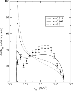
Figure 6: $s_{pp}$ distribution for an excitation energy Q=41 MeV is compared with the data form Abdel-Bary et al. zupran . In our calculation we have neglected all higher waves except the $\mbox{}^{3}P_{0}\to\mbox{}^{1}S_{0}\,s$ transition amplitude. The energy dependence in the latter is proportional to the parameter x, cf. (LABEL:t2).

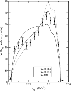
Figure 7: $s_{\eta p}$ distribution for an excitation energy Q=41 MeV is compared with the data form Abdel-Bary et al. zupran . In our calculation we have neglected all higher waves except the $\mbox{}^{3}P_{0}\to\mbox{}^{1}S_{0}\,s$ transition amplitude. The energy dependence in the latter is proportional to the parameter x, cf. (LABEL:t2).

The results of our computations are presented in Figs. 6 and 7 where they are compared with the data from zupran . In the calculation we neglected the interference terms, setting $y=z_{r}=z_{i}=0$ in (LABEL:t2). The dotted curve in Fig. 6 and Fig. 7 corresponds to a constant eta production amplitude. Whilst the $s_{\eta p}$ distribution is not too far off the experiment, the $s_{pp}$ distribution is in a bad shape as the peak caused by pp FSI is definitely much too big. The dashed curve is obtained by adopting for x the same value that for Q=15.5 MeV gave the best agreement with experiment i.e., we are pretending that this parameter does not vary with Q. This brings improvement in both cross sections and in fact the $s_{\eta p}$ distribution agrees with the data quite well. Since the parameter x may depend upon Q, and for Q=41 MeV its value could be different than for Q=15.5 MeV, we allowed x to vary, adjusting its value to the data from zupran . This time the best fit value turns out to be x=-0.863 and the corresponding distributions are presented by full curves in Figs. 6 and 7. It is not possible to improve the agreement in both distributions using the same value of the parameter x, and therefore the fit depicted by the full curve is a compromise. Although the corrections go in the right direction but the agreement is still not satisfactory and we have to accept the fact that for Q=41 MeV the assumed functional form of the cross-section is incomplete. We tried to include the interference terms with the d-waves but the fit was unsuccessful. Clearly, further extensions call for additional parameters but this does not seem to be affordable with the present data, and therefore we stop here.

Summarizing, a simple model in which the $pp\to pp\eta$ cross section contains only the dominant $\mbox{}^{3}P_{0}\to\mbox{}^{1}S_{0},s$ partial wave amplitude corrected by the final state pp interaction is capable of explaining the current experimental data at an excitation energy Q=15.5 MeV. The experimental pp and the $\eta$p effective mass distributions can be both reproduced if: (i) in the eta production amplitude a correction linear in energy is admitted and, (ii) the full pp FSI enhancement factor without the on-shell approximation is used. In the presented calculation the $\eta$p final state interaction has not been included explicitly for reasons outlined in the Introduction but since the parameters x and y have been adjusted to the data, they effectively account for this effect.