Some new perspectives on pairing in nuclei

Abstract

Following a brief reminder of how the pairing model can be solved exactly, we describe how this can be used to address two interesting issues in nuclear structure physics. One concerns the mechanism for realizing superconductivity in finite nuclei and the other concerns the role of the nucleon Pauli principle in producing $sd$ dominance in interacting boson models of nuclei.

1 Introduction

Ever since the work of Richardson in the mid-60s[1], it has been recognized that the Pairing Model (PM) is exactly solvable, even in the presence of non-degenerate single-particle levels. In recent years, there has been a resurgence of interest in the PM, with several applications reported that build on this exact solvability [2].

This talk reviews two recent applications of the PM in nuclear physics. Both build on the fact that there exists a classical electrostatic analogy for every PM. One makes use of this analogy to obtain a pictorial representation of how superconductivity arises in finite nuclear systems [3]. The other has led us to propose a new mechanism for $sd$ dominance in interacting boson models of nuclei[4].

2 Richardson’s solution of the Pairing Model

The PM hamiltonian for both fermions and bosons can be written as

$$H_{P}~{}=~{}\sum_{l}\epsilon_{l}\hat{N}_{l}~{}+~{}\frac{g}{2}\sum_{ll^{\prime}}A^{\dagger}_{l}A_{l}~{},$$ (1)

where

$$\hat{N}_{l}~{}=~{}\sum_{m}a^{\dagger}_{lm}a_{lm}~{}~{}~{},~{}~{}~{}A^{\dagger}_{l}~{}=~{}\sum_{m}a^{\dagger}_{lm}a^{\dagger}_{l\bar{m}}~{}.$$ (2)

Here $a^{\dagger}_{lm}$ creates either a boson or a fermion in single-particle state $lm$ and ${l\bar{m}}$ denotes the time reverse of $lm$.

Richardson considered the following ansatz for the ground state of a system of $2N$ particles subject to this hamiltonian:

$$|\Psi\rangle~{}=~{}\prod_{i=1}^{N}B^{\dagger}_{\alpha}~{}|0\rangle~{}~{},~{}~{}B^{\dagger}_{\alpha}~{}=~{}\sum_{l}\frac{1}{2\epsilon_{l}-e_{\alpha}}~{}A^{\dagger}_{l}~{}.$$ (3)

He showed that it is an exact eigenstate of the pairing hamiltonian if the pair energies ${\it e_{\alpha}}$ satisfy the set of equations ($\Omega_{l}=l+\frac{1}{2}$)

$$1~{}+~{}2g\sum_{l}\frac{\Omega_{l}}{2\epsilon_{l}-e_{\alpha}}~{}\mp~{}4g\sum_{\beta(\neq\alpha)}\frac{1}{e_{\beta}-e_{\alpha}}~{}=~{}0~{}.$$ (4)

In eq. (4) and throughout the presentation, the upper sign refers to boson systems and the lower sign to fermion systems.

The coupled equations (4), one for each of the $N$ collective pairs, are called the Richardson equations.

Once the set of Richardson equations has been solved, the total ground state energy of the system can be obtained by summing the resulting pair energies,

$$E~{}=~{}\sum_{\alpha}e_{\alpha}~{}.$$ (5)

While the above discussion focused on the ground state solution, it is possible to use the same general procedure to generate all excited states as well.

3 An electrostatic analogy for Pairing Models

As we have seen, the eigenvalues and eigenfunctions of the hamiltonian can be obtained using the Richardson approach, both for fermion and boson systems. From this, it is straightforward to establish an exact electrostatic analogy for the quantum pairing problem. To do so, consider the energy functional

$$U = \mp~{}\frac{1}{4g}\left[\sum_{\alpha}e_{\alpha}-\sum_{j}\Omega_{j}\epsilon_{j}\right]+\frac{1}{2}\sum_{j\alpha}(\pm\Omega_{j})\ln\left|2\epsilon_{j}-e_{\alpha}\right|$$ (6)

$$- \frac{1}{2}\sum_{\alpha\neq\beta}\ln\left|e_{\alpha}-e_{\beta}\right|-\frac{1}{8}\sum_{i\neq j}\Omega_{i}\Omega_{j}\ln\left|2\epsilon_{i}-2\epsilon_{j}\right|.$$

It can be readily shown that when we differentiate $U$ with respect to the pair energies $e_{\alpha}$ and equate to zero we recover precisely the Richardson equations (4).

To appreciate the physical meaning of $U$, we should remember that the Coulomb interaction between two point charges in two dimensions is

$$v\left({\bf r}_{1},{\bf r}_{2}\right)=-q_{1}q_{2}\ln\left|{\bf r}_{1}-{\bf r}_{2}\right|~{},$$ (7)

where $q_{i}$ is the charge and $r_{i}$ the position of particle $i$.

Thus, $U$ is the energy functional for a classical two-dimensional (2D) electrostatic system with the following ingredients:

• There are a set of fixed charges, one for each single-particle level, which are located at the positions $2\epsilon_{i}$ and have charges $\pm\frac{\Omega_{i}}{2}$. We will call them orbitons.

• There are $N$ free charges, one for each collective pair, which are located at the positions $e_{\alpha}$ and have positive unit charge. We will call them pairons.

• There is a Coulomb interaction between all charges.

• There is a uniform electric field in the vertical direction with intensity $\pm\frac{1}{4g}$.

The existence of this exact analogy suggests that we might be able to use the positions that emerge for the pairons in the classical problem to gain insight into the quantum problem, hopefully insight that was not otherwise evident.

Some other properties of the electrostatic problem that we will be using are:

• Since the orbiton positions are given by the single-particle energies, which are real, they must lie on the vertical or real axis.

• For fermion problems, the pair energies that emerge from the Richardson equations are not necessarily real. They can either be real or they can come in complex conjugate pairs. Thus, a pairon must either lie on the vertical axis (real pair energies) or be part of a mirror pair (complex pair energies).

• For boson problems, the pair energies are of necessity real and, thus, like the orbitons lie on the real axis.

4 A new pictorial representation of nuclear superconductivity

We now apply the electrostatic analogy to the problem of identical nucleon pairing and in particular to the question of how superconductivity arises in such systems. Because of the limited number of active nucleons in a nucleus, it is extremely difficult to see evidence for the transition to superconductivity in such systems.

We will discuss what happens when we apply the electrostatic analogy to the semi-magic nuclei ${}^{114-116}Sn$. The calculations are done as a function of pairing strength $g$, using single-particle energies extracted from experiment. Table 1 shows the corresponding information on the positions and charges of the orbitons.

Table 1: Position and charges of the orbitons appropriate to a pairing treatment of ${}^{114-116}Sn$.

Orbiton	Position	Charge
$d_{5/2}$	$0.0$	$-1.5$
$g_{7/2}$	$0.44$	$-2.0$
$s_{1/2}$	$3.80$	$-0.5$
$d_{3/2}$	$4.40$	$-1.0$
$h_{11/2}$	$5.60$	$-3.0$

Fig. 1 focuses on the nucleus ${}^{114}Sn$, showing the positions of the pairons in the 2D plane as a function of $g$. Since ${}^{114}Sn$ has 14 valence neutrons, there are seven pairons in the classical picture. In the limit of very weak coupling, six neutrons fill the $d_{5/2}$ orbit and eight fill the $g_{7/2}$. The corresponding electrostatic picture (Fig. 1a) has three pairons close to the $d_{5/2}$ orbiton and four close to the $g_{7/2}$. In the figure, we draw lines connecting each pairon to the one that is closest to it. These lines make clear that at very weak coupling the pairons organize themselves as artificial atoms around their corresponding orbitons.

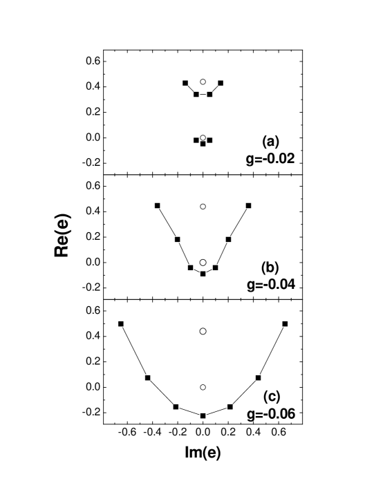
Figure 1: Two-dimensional representation of the pairon positions in ${}^{114}Sn$ for three selected values of $g$. The orbitons are represented by open circles; only the lowest two, the $d_{5/2}$ and $g_{7/2}$, are shown at the positions dictated by Table 1.

What happens as we increase the magnitude of $g$ (Figs. 1b-c)? [The physical value is roughly $-0.092~{}MeV$.] As $g$ increases, the pairons repel, causing the atoms to expand. For $g\approx-0.04$, a transition takes place from two isolated atoms to a cluster, with all pairons connected to one another. We claim that this geometrical transition from atoms to clusters in the classical problem is a reflection of the superconducting transition in the quantum problem.

We have also treated the nucleus ${}^{116}Sn$, with the same set of single-particle energies as in ${}^{114}Sn$. What we find is that in $Sn^{116}$ the transition to complete superconductivity occurs in two stages. For small $g$, the pairons distribute themselves into three atoms, surrounding the $d_{5/2}$, $g_{7/2}$ and $s_{1/2}$ orbitons. When $g$ reaches roughly $-0.06$, the two lowest atoms - containing 7 pairons - merge into a cluster, as in ${}^{114}Sn$, with the eighth still separate. When $g$ grows to roughly $-0.095$ a second transition takes place, with the eighth pairon merging into a larger cluster with the other seven. From this point on, superconductivity is complete.

5 A new mechanism for $sd$ dominance in the IBM

The electrostatic analogy can also be applied to boson pairing models, with the important caveat that the pairons are now confined to the real axis. Fig. 2 shows the pairon positions for a model involving $10$ bosons moving in all even-$L$ boson states up to $L=12$ and interacting via repulsive boson pairing with strength $g$. The single-boson energies are assumed to increase linearly with $l$.

Several points are immediately apparent. At low pairing strength, the pairons sit very near the $s$ orbiton, reflecting the fact that the bosons are almost completely in the $s$ state. As the pairing strength increases, a phase transition takes place to a scenario in which the pairons are no longer sitting near the $s$ orbiton. However, even after the phase transition all pairons are confined to the region between the lowest two orbitons, the $s$ and $d$. What this suggests is that after the phase transition the boson pairs that define the corresponding quantum ground state are most likely primarily of $s$ and $d$ character.

Figure 2: Evolution of pairons for a model involving 10 bosons in all even-$L$ states up to $L=12$ subject to a hamiltonian with linear single-boson energies and a repulsive boson pairing interaction

What is the relevance of this to the IBM? As a reminder, in the IBM the $s$ and $d$ bosons model the lowest two pair degrees of freedom for identical nucleons, those with $J^{\pi}=2^{+}$ and $4^{+}$. The key assumption of the model is that all other bosons, reflecting higher pair states, can be ignored, except for their renormalization effects. A second point to remember is that in any effort to model composite objects by structureless particles, there invariably arises a repulsive interaction between these particles, to reflect the Pauli exchange between their constituents.

The results in Fig. 2 are suggestive that in the presence of such a repulsive interaction between bosons only the two lowest boson degrees of freedom can correlate, namely the $s$ and $d$. This suggests that repulsive pairing between bosons provides a new mechanism for $sd$ dominance in interacting boson models of nuclei.

Figure 3: Occupation probabilities for the ground state of a system of $5$ boson pairs and maximum angular momentum $L=12$ as a function of the $g$. The upper graph shows the sum of occupation probabilities (depletion) for high-spin bosons ($l>2$) while the lower graph gives the occupation probabilities for $s$ and $d$ bosons. The dashed lines refer to Model I and the solid line4s to Model II, as described in the text.

These points can be made more quantitative by looking directly at the quantum results. In Fig. 3, we show results for the same interacting boson model as above, but now with two possible choices for the single-boson spectrum. In addition to the choice $\epsilon_{l}=l$ used before (Model I), we also consider $\epsilon_{l}=l^{2}$ (Model II). In this way, we can assess whether $sd$ dominance is a general feature of boson models involving repulsive pairing or is limited to the model earlier shown.

As we can see from the figure, both models show the same general features. For weak $g$, most of the bosons are in the $s$ state. As $g$ increases, there is a phase transition to a mixed or fragmented state. However, even in the fragmented state there are essentially no bosons other than those with $L=0$ and $2$.

Indeed, when we carry out the calculation as a function of boson number, we find that as $N$ grows the number of non-$sd$ bosons decreases, and in the thermodynamic limit there are only $s$ and $d$ bosons.

6 Summary

There are two key points we have tried to get across in this presentation. The first is that pairing models, even with non-degenerate levels, can be solved exactly using a method introduced by Richardson almost 40 years ago. The second is that these exactly solvable models can be used to provide interesting insight into several issues of importance in nuclear physics. The two examples we discussed concerned the mechanism for realizing superconductivity in finite nuclear systems and the role of the nucleon Pauli principle in producing $sd$ dominance in interacting boson models of nuclei.

References

- [1] R.W. Richardson, Phys. Lett. 3, 277 (1963); R.W. Richardson and N. Sherman, Nucl. Phys. 52, 221 (1964); R.W. Richardson, J. Math. Phys. 9, 1327 (1968).
- [2] G. Sierra, J. Dukelsky, G.G. Dussel, J. von Delft and F. Braun, Phys. Rev. B 61, R11890 (2000).
- [3] J. Dukelsky, C. Esebbag and S. Pittel, Phys. Rev. Lett. 88 (2002) 062501.
- [4] J. Dukelsky and S. Pittel, Phys. Rev. Lett. 86 (2001) 4791.