Proton-rich Nuclei at and beyond the Proton Drip Line in the Relativistic Mean Field Theory

Abstract

Ground state properties of proton-rich odd-$Z$ nuclei in the region $55\leq Z\leq 73$ are studied in the relativistic mean field (RMF) theory. The RMF equations are solved by using the expansion method in the Harmonic-Oscillator basis. In the particle-particle channel, we use the state-dependent BCS method with a zero-range $\delta$-force, which has been proved to be effective even for neutron-rich nuclei. All the ground state properties, including the one-proton separation energies, the ground state deformations, the last occupied proton orbits and the locations of proton drip line, are calculated. Good agreement with both the available experimental data and the predictions of the RHB method are obtained.

1 Introduction

The structure and decay modes of nuclei at and beyond the proton drip line represent one of the most active areas in both experimental and theoretical studies of exotic nuclei with extreme isospin ratios. Recent reviews can be found in Refs. [1, 2] and references therein. For each element, the number of neutrons that can be supported by the nucleus is limited if the nucleus is to remain stable with respect to nucleonic emission. These limits define the proton and neutron drip lines. The main difference between the proton and the neutron is the existence of the Coulomb potential for the former. Consequently, the proton drip line lies much closer to the stability line than the neutron drip line. For example, the lightest particle-stable neon isotope is ${}^{17}_{10}$Ne₇ [1] , while as heavy an isotope as ${}^{34}_{10}$Ne₂₄ [3] is known to exist. The existence of the Coulomb barrier also traps the wave function of the proton in the nuclear region, which explains why we have not yet clearly observed halo phenomena in proton-rich nuclei.

The proton drip line has been almost fully mapped up to $Z=21$ [1] experimentally. No proton-unbound nuclei have been directly observed in this region, which is not surprising, since the Coulomb barrier is relatively low. It has been argued that ground state proton decay can only be detected directly for nuclei with $Z>50$, where the relatively high potential energy barrier causes nuclei to survive long enough to be detected experimentally [1]. Detailed studies of ground state proton radioactivity have been reported for odd-$Z$ nuclei mainly in the two mass regions, $51\leq Z\leq 55$ and $69\leq Z\leq 83$. The experimental features observed for most of these nuclei have been explained by assuming them to have spherical shapes [2]. The half-lives for proton decay were then evaluated using the semi-classical WKB method or standard reaction theory within the distorted wave approximation. However, to obtain proton decay rates in the transitional region beyond the $Z=50$ shell closure (¹⁰⁹I and ^112,113Cs) and in the region of light rare-earth nuclei (¹³¹Eu and ^140,141Ho) requires calculations assuming significant prolate deformations. Recently, an exact formalism was developed in Refs. [4, 5], where the half-lives are evaluated with the assumption that the emitted proton exists in a deformed single particle Nilsson level. This formalism was applied [4, 5, 6, 7] to analyze all data presently available for odd proton emitters with an even number of neutrons and the known odd-odd proton emitters ¹¹²Cs, ¹⁴⁰Ho and ¹⁵⁰Lu [8]. This formalism, however, does not predict proton separation energies, i.e. the model does not predict which nuclei are likely to be proton emitters.

In the past decade, the relativistic mean field (RMF) theory has been successfully applied to the study of nuclear properties throughout the Periodic Table. General reviews of the RMF theory and its applications in nuclear physics can be found in Refs. [9, 10, 11, 12]. To study exotic nuclei whose Fermi surfaces are close to the threshold, several issues, including the continuum and the pairing correlation, must be treated carefully [13, 14, 15, 16, 17, 18, 19, 20]. Luckily, in the case of proton-rich nuclei, because the nuclear wave function is well confined in the nuclear region due to the existence of the Coulomb potential, one only needs to take care of the pairing correlation. The use of a zero-range $\delta$-force in the particle-particle channel, $V=-V_{0}\delta({\vec{r}_{1}}-{\vec{r}_{2}})$, has proved to be an efficient and economical way to accomplish this [13, 14, 15, 16, 17, 18, 19, 20]. (For detailed discussions of more general cases, including neutron-rich nuclei, we refer the reader to Refs. ^13)-20) and references therein.) In our present work, the deformed RMF+BCS method with a zero-range $\delta$-force in the pairing channel [20, 21, 22] is applied to the analysis of deformed odd-$Z$ proton-rich nuclei with $55\leq Z\leq 73$. In the mean-field part, two of the most successful parameter sets, TMA [23] and NL3, [24] are used.

The RMF theory was first applied to study deformed proton emitters by Lalazissis et al. In Refs. [25, 26, 27, 28], the proton drip-line nuclei with $31\leq Z\leq 49$ and $51\leq Z\leq 73$ are studied within the framework of the Relativistic Hartree-Bogoliubov (RHB) model. In the mean-field part, the NL3 [24] parameter set is used. In the particle-particle channel, the pairing part of the Gogny force with the D1S set [29] has been adopted. The calculated one-proton separation energy and other relevant properties are in good agreement with the available experimental data. Such a success shows that the RMF theory could be an appropriate method even for the description of nuclei with extreme isospin ratios. This observation also motivates us to study deformed proton emitters within a different framework, that of the deformed RMF+BCS method, due to the following considerations. First, we would like to see whether such a success is dependent on the choice of a particular combination of parameter sets, i.e. NL3+D1S. Second, we want to see whether the argument that a zero-range $\delta$-force is an efficient and economical interaction to treat the pairing correlation holds in such extreme cases, i.e. at and/or near the proton drip line. Finally, many new theoretical and experimental works, including those reported in Refs. [6, 8, 30, 31], to name just a few, have been carried out since the last series of works [25, 26, 27, 28] in the relativistic mean field theory. Because in general, the BCS method is thought of as an approximation to the full Bogoliubov transformation, we would like to compare our results with the existing RHB results.

The article is organized as follows. In §2, we give a brief introduction to the deformed RMF+BCS method. In §3, we present our results for odd-$Z$ proton-rich nuclei with $55\leq Z\leq 73$ and compare our results with the available experimental data and those of the RHB method. §4 is devoted to the summary of this paper.

2 The deformed RMF+BCS method

Our RMF calculations have been carried out using the model Lagrangian density with nonlinear terms both for the $\sigma$ and $\omega$ mesons, as described in detail in Ref. [20]. The Lagrangian density is given by

$${\cal L} = \bar{\psi}(i\gamma^{\mu}\partial_{\mu}-M)\psi+\,\frac{\displaystyle 1}{\displaystyle 2}\partial_{\mu}\sigma\partial^{\mu}\sigma-\frac{\displaystyle 1}{\displaystyle 2}m_{\sigma}^{2}\sigma^{2}-\frac{\displaystyle 1}{\displaystyle 3}g_{2}\sigma^{3}-\frac{\displaystyle 1}{\displaystyle 4}g_{3}\sigma^{4}-g_{\sigma}\bar{\psi}\sigma\psi$$ (1)

$$-\frac{\displaystyle 1}{\displaystyle 4}\Omega_{\mu\nu}\Omega^{\mu\nu}+\frac{\displaystyle 1}{\displaystyle 2}m_{\omega}^{2}\omega_{\mu}\omega^{\mu}+\frac{\displaystyle 1}{\displaystyle 4}g_{4}(\omega_{\mu}\omega^{\mu})^{2}-g_{\omega}\bar{\psi}\gamma^{\mu}\psi\omega_{\mu}$$

$$-\frac{\displaystyle 1}{\displaystyle 4}{R^{a}}_{\mu\nu}{R^{a}}^{\mu\nu}+\frac{\displaystyle 1}{\displaystyle 2}m_{\rho}^{2}\rho^{a}_{\mu}\rho^{a\mu}-g_{\rho}\bar{\psi}\gamma_{\mu}\tau^{a}\psi\rho^{\mu a}$$

$$-\frac{\displaystyle 1}{\displaystyle 4}F_{\mu\nu}F^{\mu\nu}-e\bar{\psi}\gamma_{\mu}\frac{\displaystyle 1-\tau_{3}}{\displaystyle 2}A^{\mu}\psi,$$

where the field tensors of the vector mesons and of the electromagnetic field take the forms

$$\left\{\begin{array}[]{rl}\Omega_{\mu\nu}=&\partial_{\mu}\omega_{\nu}-\partial_{\nu}\omega_{\mu},\\ R^{a}_{\mu\nu}=&\partial_{\mu}\rho^{a}_{\nu}-\partial_{\nu}\rho^{a}_{\mu}-2g_{\rho}\epsilon^{abc}\rho^{b}_{\mu}\rho^{c}_{\nu},\\ F_{\mu\nu}=&\partial_{\mu}A_{\nu}-\partial_{\nu}A_{\mu},\end{array}\right.$$ (2)

and other symbols have their usual meanings. Based on the single-particle spectra calculated with the RMF method, we perform a state-dependent BCS calculation [32, 33]. The gap equation has a standard form for all the single particle states,

$$\Delta_{k}=-\frac{\displaystyle 1}{\displaystyle 2}\sum_{k^{\prime}>0}\frac{\displaystyle\bar{V}_{kk^{\prime}}\Delta_{k^{\prime}}}{\displaystyle\sqrt{(\varepsilon_{k^{\prime}}-\lambda)^{2}+\Delta_{k^{\prime}}^{2}}},$$ (3)

where $\varepsilon_{k^{\prime}}$ is the single particle energy and $\lambda$ is the Fermi energy, whereas the particle number condition is given by $2\sum\limits_{k>0}v_{k}^{2}=N$. In the present work, for the pairing interaction we use a zero-range $\delta$-force,

$$V=-V_{0}\delta({\vec{r}_{1}}-{\vec{r}_{2}}),$$ (4)

with the same strength $V_{0}$ for both protons and neutrons. The pairing matrix element for the zero-range $\delta$-force is given by

$$\begin{array}[]{lll}\bar{V}_{ij}&=&\langle i\bar{i}|V|j\bar{j}\rangle-\langle i\bar{i}|V|\bar{j}j\rangle=-V_{0}\int d^{3}r\,\left[\psi^{\dagger}_{i}\psi^{\dagger}_{\bar{i}}\psi_{j}\psi_{\bar{j}}-\psi^{\dagger}_{i}\psi^{\dagger}_{\bar{i}}\psi_{\bar{j}}\psi_{j}\right],\\ \end{array}$$ (5)

with the nucleon wave function in the form

$$\psi_{i}({\vec{r}},t)=\left(\begin{array}[]{c}f_{i}({\vec{r}})\\ ig_{i}({\vec{r}})\end{array}\right)=\frac{\displaystyle 1}{\displaystyle\sqrt{2\pi}}\left(\begin{array}[]{l}f^{+}_{i}(z,r_{\bot})e^{i(\Omega_{i}-1/2)\varphi}\\ f^{-}_{i}(z,r_{\bot})e^{i(\Omega_{i}+1/2)\varphi}\\ ig^{+}_{i}(z,r_{\bot})e^{i(\Omega_{i}-1/2)\varphi}\\ ig^{-}_{i}(z,r_{\bot})e^{i(\Omega_{i}+1/2)\varphi}\end{array}\right)\chi_{t_{i}}(t).$$ (6)

A detailed description of the deformed RMF+BCS method can be found in Ref. [20].

In the present study, nuclei with both even and odd numbers of protons (neutrons) need to be calculated. We adopt a simple blocking method, in which the ground state of an odd system is described by the wave function

$$\alpha^{\dagger}_{k_{1}}|\textrm{BCS}\rangle=\alpha^{\dagger}_{k_{1}}\prod_{k\neq k_{1}}(u_{k}+v_{k}\alpha^{\dagger}_{k}\alpha^{\dagger}_{\bar{k}})|\textrm{vac}\rangle.$$ (7)

Here, $|\textrm{vac}\rangle$ denotes the vacuum state. The unpaired particle sits in the level $k_{1}$ and blocks this level from pairing correlations. The Pauli principle prevents this level from participating in the scattering process of nucleons caused by the pairing correlations. As described in Ref. [33], in the calculation of the gap, one level is “blocked”,

$$\Delta_{k}=-\frac{\displaystyle 1}{\displaystyle 2}\sum_{k^{\prime}\neq k_{1}>0}\frac{\displaystyle\bar{V}_{kk^{\prime}}\Delta_{k^{\prime}}}{\displaystyle\sqrt{(\varepsilon_{k^{\prime}}-\lambda)^{2}+\Delta_{k^{\prime}}^{2}}}.$$ (8)

The level $k_{1}$ has to be excluded from the sum, because it cannot contribute to the pairing energy. The corresponding chemical potential, $\lambda$, is determined by

$$N=1+2\sum_{k\neq k_{1}>0}v^{2}_{k}.$$ (9)

This blocking procedure is performed at each step of the self-consistent iteration.

3 Deformed ground-state proton emitters with $55\leq Z\leq 73$

In the present work, we use the mass-dependent parameter set TMA [23] for the RMF Lagrangian. Results with the parameter set NL3 [24] are also presented for comparison. For each nucleus, first the quadrupole constrained calculation [34, 35] is performed to obtain all possible ground state configurations, and then we perform the non-constrained calculation using the quadrupole deformation parameter of the deepest minimum of the energy curve of each nucleus as the deformation parameter for our Harmonic-Oscillator basis. In the case that there are several similar minima obtained from the constrained calculation, we repeat the above-described procedure to obtain the configuration with the lowest energy as our final result. The calculations for the present analysis have been performed using an expansion in 14 oscillator shells for fermion fields and 20 shells for boson fields for isotopes with $Z\geq 70$, i.e. Ta and Lu isotopes. While for isotopes with $Z\leq 70$, 12 shells for fermion fields and 20 shells for boson fields are used. In the latter case, we use 12 shells for fermions to save computation time. Convergence has been tested for all the quantities calculated here. Following Ref. [36], we fix $\hbar\omega_{0}=41A^{-1/3}$ for fermions.

Whenever the zero-range $\delta$ force is used in the BCS framework, a cutoff procedure must be applied, i.e. the space of the single-particle states in which the pairing interaction acts must be truncated. This is not only to simplify the numerical calculation but also to simulate the finite-range (more precisely, long-range) nature of the pairing interaction in a phenomenological way [37, 38]. In the present work, the single-particle states subject to the pairing interaction are confined to the region satisfying

$$\epsilon_{i}-\lambda\leq E_{\mathrm{cut}},$$ (10)

where $\epsilon_{i}$ is the single-particle energy, $\lambda$ the Fermi energy, and $E_{\mathrm{cut}}=8.0$ MeV. We find that increasing $E_{\mathrm{cut}}$ from 8.0 MeV up to 16.0 MeV, followed by a readjustment of the pairing strength $V_{0}$, does not change the results, and therefore none of our conclusions will change. The same pairing strength is used for both protons and neutrons and is fixed by requiring that the experimental one-proton separation energies of several selected nuclei be reproduced by our calculations, including ¹⁵⁷Ta, ¹⁴⁷Tm, and ¹¹¹Cs. A slight readjustment of the pairing strength, say %5 , does not change our conclusion here. More specifically, for calculations with the NL3 set, we take $V_{0}=393.0$ MeV fm³ for $Z\geq 71$, and $V_{0}=420.0$ MeV fm³ otherwise. For calculations with the TMA set, we take $V_{0}=393.0$ MeV fm³ for $Z\geq 71$, and $V_{0}=375.0$ MeV fm³ otherwise. We should mention that the small difference between $V_{0}$ for isotopes with $Z\geq 71$ and isotopes with $Z<71$ is partly due to the different number of shells used in the expansion method.

In the process of proton emission, the valence proton tunnels through the Coulomb and centrifugal barriers, and the decay probability depends strongly on the energy of the unbound proton and on its angular momentum. In rare-earth nuclei, the decay of the ground state by direct proton emission competes with $\beta^{+}$ decay; for heavy nuclei, fission or $\alpha$-decay can also be favored. In general, ground state proton emission is not observed immediately beyond the proton drip line. For small values of the proton separation energy, the width is dominated by $\beta^{+}$ decay. On the other hand, large separation energies result in extremely short proton emission half-lives, which are difficult to observe experimentally. For a typical rare-earth nucleus, the separation energy window, in which ground state proton decay can be directly observed, is about 0.8–1.7 MeV [2].

The Nilsson quantum numbers of the last occupied proton orbit are taken to be the same as the dominant component in the expansion of this wave function in terms of the axially-symmetric Harmonic-Oscillator basis [36]. In theoretical calculations, the spectroscopic factor of the corresponding odd-proton orbit, $k$, is defined as the probability that this orbit is found empty in the daughter nucleus with one less proton [26]. If the difference between the ground state configurations of the mother and the daughter nuclei is ignored, the spectroscopic factor for level $k$ is calculated as

$$S_{k}=|\langle\phi|\alpha_{k}|\phi_{k}\rangle|^{2}=u^{2}_{k}.$$ (11)

Here, $u^{2}_{k}$ is related to the occupation probability $v^{2}_{k}$ for level $k$ in the daughter nucleus through the well-known relation in the BCS formalism

$$u^{2}_{k}+v^{2}_{k}=1.$$ (12)

In what follows, we discuss the details of our numerical results.

3.1 Lutetium (Z=71) and Tantalum (Z=73)

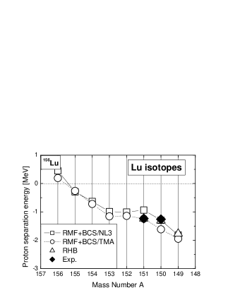
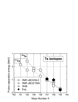
Figure 1: The one-proton separation energies for Lu ($Z$=71) and Ta ($Z$=73) isotopes at and beyond the proton drip line. The experimental value for the proton separation energy corresponds to the opposite of the ground state transition energy, $E_{p}$.

The one-proton separation energies for Lu and Ta isotopes are displayed in Fig. 1 as functions of the mass number A. The drip-line nucleus for the Ta isotopic chain is predcited to be ¹⁶⁰Ta by NL3 and ¹⁶¹Ta by TMA. While for the Lu isotopic chain, both TMA and NL3 predict the drip-line nucleus to be ¹⁵⁶Lu. We also compare the calculated separation energies with the available experimental transition energies for ground state proton emission in ¹⁵⁰Lu, ¹⁵¹Lu [40], ¹⁵⁵Ta [41], ¹⁵⁶Ta [42] and ¹⁵⁷Ta [43]. The corresponding RHB results are taken from Ref. [25]. In Table I, we list the ground state properties of Lu and Ta isotopes. The separation energy window, 0.8–1.7 MeV, extends to include those nuclei for which a direct observation of ground state proton emission is in principle possible on the basis of our calculated separation energies. Good agreement between our calculations and both the experimental data and the RHB results is clearly seen. However, for the odd-odd nuclei ¹⁵⁰Lu and ¹⁵⁶Ta, our calculations predict values of $S_{p}$ smaller than the experimental values. This may be explained by the possible existence of a residual proton-neutron pairing interaction. In both nuclei, an extra positive energy of about $0.3$ MeV is needed to increase the calculated $S_{p}$ value to the experimental value. We find that if we reduce the pairing strength for odd-odd nuclei by about 5–10% compared with odd-even or even-even nuclei, we can fit the experimental transition energy quite well. We see below that the same conclusion also holds for other odd-odd nuclei. Although it has long been known that the proton-neutron pairing is important for the proper description of nuclei [44, 45], it was believed that it only affects those proton-rich nuclei with $N\approx Z$. However, recently Šimkovic et al. [46] showed that even for nuclei with $N-Z=12$, the proton-neutron pairing cannot be ignored.

Table 1: Lu ($Z$=71) and Ta ($Z$=73) ground state proton emitters. The results of RMF+BCS/TMA calculations (third to sixth columns) for the one-proton separation energy, $S_{p}$, the mass quadrupole deformation, $\beta_{2}$, and the deformed single-particle orbit occupied by the odd valence proton, are compared with the predictions of the RHB model [25, 26] (seventh to tenth columns) and with the experimental values, $S_{p}=-E_{p}$, where $E_{p}$ is the experimental transition energy. The RMF+BCS/TMA and RHB spectroscopic factors are displayed in the sixth and tenth columns, respectively. All energies are in units of MeV.

		RMF+BCS/TMA				RHB				Exp.
	$N$	$S_{p}$	$\beta_{2}$	p orbital	$u^{2}$	$S_{p}$	$\beta_{2}$	p orbital	$u^{2}$	$S_{p}$
149Lu	78	$-1.946$	$-0.166$	$5/2^{-}$[512]	0.574	$-1.77$	$-0.158$	$7/2^{-}$[523]	0.60
150Lu	79	$-1.613$	$-0.129$	$5/2^{-}$[523]	0.549	$-1.31$	$-0.153$	$7/2^{-}$[523]	0.61	$-1.261$(4) [40]
151Lu	80	$-1.239$	$-0.119$	$5/2^{-}$[532]	0.541	$-1.24$	$-0.151$	$7/2^{-}$[523]	0.58	$-1.233$(3) [40]
152Lu	81	$-1.141$	$-0.053$	$5/2^{-}$[532]	0.496
153Lu	82	$-1.156$	0.002	$7/2^{-}$[523]	0.463
154Lu	83	$-0.720$	$-0.050$	$5/2^{-}$[532]	0.513
155Ta	82	$-1.698$	0.007	$9/2^{-}$[514]	0.374	$-1.677$	0.000	$11/2^{-}$	0.60	$-1.765$(10) [41]
156Ta	83	$-1.462$	$-0.048$	$3/2^{-}$[521]	0.437	$-1.129$	0.000	$3/2^{+}$	0.51	$-1.007$(5) [42]
157Ta	84	$-0.974$	0.036	$9/2^{-}$[514]	0.381	$-1.040$	0.000	$11/2^{-}$	0.42	$-0.927$(7) [43]
158Ta	85	$-0.725$	0.077	$9/2^{-}$[514]	0.470

With regard to the deformation, both our RMF+BCS method and the RHB model predict oblate shapes for Lu proton emitters and similar values for the ground state quadrupole deformations. Recent calculations by Ferreira et al. [6] show that the proton decay in ¹⁵¹Lu can be described very well as a decay from a $K=5/2^{-}$ ground state with an oblate deformation for which $-0.18<\beta_{2}<-0.14$. In another work [8], the author finds that the proton decay in ¹⁵⁰Lu is described very well as a decay from a $K=5/2^{-}$ ground state with an oblate deformation satisfying $-0.17<\beta_{2}<-0.16$. These calculations are in reasonable agreement with our predictions (see Table I). While the RHB method [25] predicts that the last occupied orbit is $7/2^{-}[523]$ for both nuclei. If we look into the single-particle spectra of these two nuclei more closely, we find that in addition to the $5/2^{-}$ possibilities, which are listed in Table I, the orbits $1/2^{+}[400]$ and $7/2^{-}[523]$ are also possibly blocked. The total energy difference between these blocking choices are $E_{5/2}-E_{1/2}=0.061$ MeV and $E_{5/2}-E_{7/2}=0.303$ MeV for ¹⁵¹Lu; $E_{5/2}-E_{1/2}=-0.040$ MeV and $E_{5/2}-E_{7/2}=0.242$ MeV for ¹⁵⁰Lu, where $E$ is the binding energy for our calculations with the TMA parameter set.

In calculations using the RHB model [25], Ta isotopes are assumed to be spherical, while they are slightly deformed in our calculations. At first sight, the RMF+BCS/TMA and RHB models seem to predict quite different $p$–orbitals for ¹⁵⁷Ta, ¹⁵⁶Ta, and ¹⁵⁵Ta, but in fact these states are quite close in our calculations. The theoretical predictions are compared with the corresponding experimental assignments for the ground state configuration and spectroscopic factor. The experimental data for ¹⁵⁵Ta [41], ¹⁵⁶Ta [2] and ¹⁵⁷Ta [2] are, respectively, the $p$–orbital $11/2^{-}$ with 0.58(20), the $p$–orbital $3/2^{+}$ with 0.67(16) and the $p$–orbital $1/2^{+}$ with 0.74(34). We notice that the experimental assignments are somewhat different both from our predictions, in which ^155-157Ta are slightly deformed, and from the RHB calculations, in which spherical shapes are assumed. There are two possible explanations for this disagreement. First, these states are close to each other in our calculations and therefore it is difficult to make a clear distinction between them. Second, deformation could slightly change the state occupied by the odd-proton. Because the nuclei ^155-157Ta are not strongly deformed, a different combination of deformation and the occupied state can give the same experimentally observed values, i.e. the experimental transition energies and decay half-lives.

3.2 Holmium (Z=67) and Thulium (Z=69)

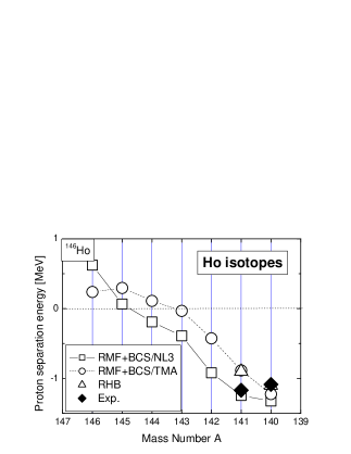
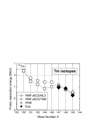
Figure 2: The same as Fig. 1, but for Ho ($Z$=67) and Tm ($Z$=69) isotopes.

Table 2: The same as Table 1, but for Ho ($Z$=67) and Tm ($Z$=69) isotopes.

		RMF+BCS/TMA				RHB				Exp.
	$N$	$S_{p}$	$\beta_{2}$	p orbital	$u^{2}$	$S_{p}$	$\beta_{2}$	p orbital	$u^{2}$	$S_{p}$
140Ho	73	$-1.223$	0.341	$7/2^{-}[523]$	0.592	$-1.10$	0.31	$7/2^{-}$[523]	0.61	$-1.086$(10) [49]
141Ho	74	$-0.885$	0.339	$7/2^{-}[523]$	0.594	$-0.90$	0.32	$7/2^{-}$[523]	0.64	$-1.169$(8) [50]
145Tm	76	$-1.458$	$-0.220$	$7/2^{-}[523]$	0.458	$-1.43$	0.23	$7/2^{-}$[523]	0.47	$-1.728$(10) [48]
146Tm	77	$-1.238$	$-0.207$	$7/2^{-}[523]$	0.460	$-1.20$	$-0.21$	$7/2^{-}$[523]	0.50	$-1.120$(10) [47]
147Tm	78	$-0.958$	$-0.186$	$7/2^{-}[523]$	0.467	$-0.96$	$-0.19$	$7/2^{-}$[523]	0.55	$-1.054$(19) [40]

In Fig. 2, we plot the one-proton separation energies for Ho and Tm isotopes as functions of the mass number A. The available experimental data for ¹⁴⁷Tm [40], ¹⁴⁶Tm [47], ¹⁴⁵Tm [48], ¹⁴⁰Ho [49] and ¹⁴¹Ho [50], together with the results of the RHB calculations [26], are also shown for comparison. The predicted drip-line nucleus for the Tm isotopic chain is ¹⁵²Tm, while for the Ho isotopic chain, NL3 predicts ¹⁴⁶Ho and TMA predicts ¹⁴⁴Ho. From Fig. 2, we can see that both RMF+BCS/TMA and RHB predict a smaller transition energy for ¹⁴¹Ho, while RMF+BCS/NL3 predicts a value of $S_{p}$ that is closer to the experimental value. Nevertheless, all theoretical calculations fail to predict the increase of the one-proton separation energy from ¹⁴¹Ho to ¹⁴⁰Ho. This can be corrected by reducing the pairing strength by a few percent, as discussed above. However, this is not our aim here. It is quite clear that, even after changing the pairing strength, we cannot account for the trend from ¹⁴¹Ho to ¹⁴⁰Ho, which has been attributed to the lack of a residual proton-neutron interaction in our above analysis. In Table II, we list the properties of the Ho and Tm proton emitters. We note that our RMF+BCS/TMA calculations predict an oblate shape for ¹⁴⁵Tm, while the RHB method predicts a prolate shape. In fact, in our constrained calculation, both prolate and oblate shapes are possible for ¹⁴⁵Tm and ¹⁴⁴Er. This is illustrated in Fig. 3, where we plot the binding energy per particle for ¹⁴⁵Tm and ¹⁴⁴Er as functions of the quadrupole deformation parameter, $\beta_{2m}$. The binding energies are obtained from the RMF+BCS/TMA calculations performed by imposing a quadratic constraint on the quadrupole moment. We find two similar minima around $\beta_{2}\approx-0.22$ and $\beta_{2}\approx 0.25$ for both ¹⁴⁵Tm and ¹⁴⁴Er. More specifically, for ¹⁴⁵Tm the two minima are $E/A=-7.906$ at $\beta_{2m}=0.287$ and $E/A=-7.903$ at $\beta_{2m}=-0.211$, while for ¹⁴⁴Er they are $E/A=-7.767$ at $\beta_{2m}=0.303$ and $E/A=-7.768$ at $\beta_{2m}=-0.196$. The reason that we choose the oblate shape instead of the prolate shape for ¹⁴⁵Tm is two-fold. First, we would like to choose the same shape for both ¹⁴⁵Tm and ¹⁴⁴Er. Second, the oblate shape for ¹⁴⁵Tm is more consistent with its neighbors (also see Fig. 7). We note that, unlike Lu and Ta isotopes, here both RMF+BCS/TMA and RHB predict the same last occupied odd-proton state for Ho and Tm isotopes (also see Table II).

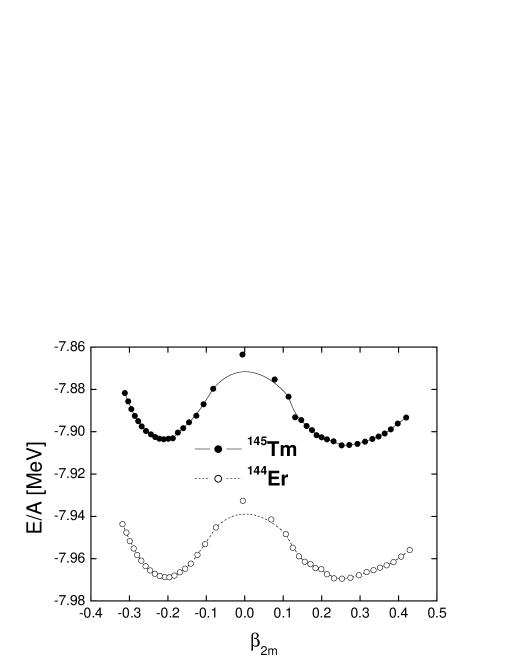
Figure 3: Binding energy per particle, $E/A$, for ¹⁴⁵Tm and ¹⁴⁴Er, plotted as functions of the mass quadrupole deformation parameter, $\beta_{2m}$.

3.3 Europium (Z=63) and Terbium (Z=65)

Figure 4: The same as Fig. 1, but for Eu ($Z$=63) and Tb ($Z$=65) isotopes.

In Fig. 4, we plot the one-proton separation energies for Tb and Eu isotopes. The results of the RHB model [26] and the only available experimental data for ¹³¹Eu [50] are also shown. The drip-line nucleus for the Tb isotopic chain is predicted to be ¹⁴⁰Tb by NL3 and to be ¹³⁹Tb by TMA. While for the Eu isotopic chain, the drip-line nucleus is predicted to be ¹³³Eu by TMA and ¹³⁴Eu by NL3. In this region, only one proton emitter, ¹³¹Eu, has been reported. However, based on our calculations, there are three other possible proton emitters, ¹³⁰Eu, ¹³⁵Tb and ¹³⁶Tb. We list their properties in Table 3. We notice that the experimental transition energy for ¹³¹Eu is 0.950(8) MeV, while our RMF+BCS/TMA calculations predict 0.498 MeV. This can be corrected by adjusting the pairing strength slightly. Considering this correction, we see that RHB and RMF+BCS predict similar proton emitters for Tb and Eu isotopes. As we have seen from the results presented to this point, the description of proton emitters is quite sensitive to the pairing strength. We hope that further experimental measurements of proton emitters in the entire region can help us understand more about the pairing interaction in exotic nuclei.

Table 3: The same as Table 1, but for Eu ($Z$=63) and Tb ($Z$=65) isotopes.

		RMF+BCS/TMA				RHB				Exp.
	$N$	$S_{p}$	$\beta_{2}$	p orbital	$u^{2}$	$S_{p}$	$\beta_{2}$	p orbital	$u^{2}$	$S_{p}$
130Eu	67	$-0.778$	0.420	$5/2^{+}[413]$	0.464	$-1.22$	0.34	$5/2^{-}$[532]	0.44
131Eu	78	$-0.498$	0.411	$5/2^{+}[413]$	0.323	$-0.90$	0.35	$5/2^{+}$[413]	0.44	$-0.950$(8) [50]
135Tb	70	$-1.010$	0.365	$3/2^{+}[411]$	0.879	$-1.15$	0.34	$3/2^{+}$[411]	0.62
136Tb	71	$-0.653$	0.374	$3/2^{+}[411]$	0.862	$-0.90$	0.32	$3/2^{+}$[411]	0.65

3.4 Praseodymium (Z=59) and Promethium (Z=61)

In Fig. 5, the one-proton separation energies for Pm and Pr isotopes are plotted as functions of the mass number A, together with the results of the RHB model [26]. The drip-line nuclei are predicted to be ¹²⁸Pm and ¹²⁵Pr by both TMA and NL3. No experimental proton emitters have been reported for these two isotopic chains. Based on our calculations, possible proton emitters in this region are ^119,120Pr and ^124,125Pm. The properties of these nuclei are listed in Table IV.

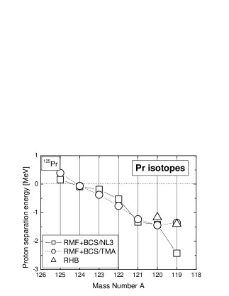
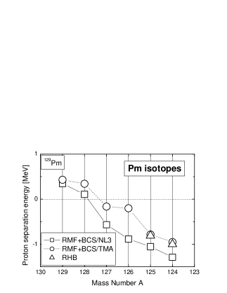
Figure 5: The same as Fig. 1, but for Pr ($Z$=59) and Pm ($Z$=61) isotopes.

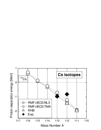
Figure 6: The same as Fig. 1, but for Cs ($Z$=55) and La ($Z$=57) isotopes.

3.5 Cesium (Z=55) and Lanthanum (Z=57)

In Fig. 6, we plot the one-proton separation energies for Cs and La isotopes. The results of the RHB model [26] are also shown for comparison. The drip-line nuclei are predicted to be ¹¹⁵Cs and ¹¹⁸La by TMA, ¹¹⁵Cs and ¹¹⁹La by NL3. In Fig. 6, we see that the latest reported proton emitter, ¹¹⁷La [30, 31], is reproduced quite well by RMF+BCS/NL3 calculations. Both RHB and RMF+BCS fail to reproduce the experimental data for ¹¹²Cs. As mentioned above, ¹¹²Cs has an odd number of protons and an odd number of neutrons. Since $N-Z$ is only 2, we expect a relatively strong interaction between the odd proton and the odd neutron. Compared with an odd-even system, the additional interaction increases the binding energy somewhat. Because the two mean-field models, RHB and RMF+BCS, do not include any residual proton-neutron interaction, they cannot reproduce the inversion of separation energies. Also, it is suggested in Ref. [26] that such an additional interaction could be represented by a surface delta-function interaction. According to our calculations, the remaining possible proton emitters in the La isotopic chain are ¹¹⁵La and ¹¹⁶La, as listed in Table V.

Table 4: The same as Table 1, but for Pr ($Z$=59) and Pm ($Z$=61) isotopes.

		RMF+BCS/TMA				RHB				Exp.
	$N$	$S_{p}$	$\beta_{2}$	p orbital	$u^{2}$	$S_{p}$	$\beta_{2}$	p orbital	$u^{2}$	$S_{p}$
119Pr	60	$-1.354$	0.381	$3/2^{-}$[541]	0.436	$-1.40$	0.32	$3/2^{-}$[541]	0.39
120Pr	61	$-1.445$	0.442	$9/2^{+}$[404]	0.107	$-1.17$	0.33	$3/2^{-}$[541]	0.33
124Pm	63	$-0.950$	0.422	$5/2^{-}$[532]	0.789	$-1.00$	0.35	$5/2^{-}$[532]	0.72
125Pm	64	$-0.783$	0.412	$5/2^{-}$[532]	0.800	$-0.81$	0.35	$5/2^{-}$[532]	0.74

Table 5: The same as Table 1, but for Cs ($Z$=55) and La ($Z$=57) isotopes.

		RMF+BCS/TMA				RHB				Exp.
	$N$	$S_{p}$	$\beta_{2}$	p orbital	$u^{2}$	$S_{p}$	$\beta_{2}$	p orbital	$u^{2}$	$S_{p}$
111Cs	56	$-1.913$	0.206	$1/2^{+}$[420]	0.949	$-1.97$	0.20	$1/2^{+}$[420]	0.74
112Cs	57	$-1.213$	0.171	$5/2^{+}$[413]	0.906	$-1.46$	0.20	$1/2^{+}$[420]	0.74	$-0.807$(7) [51]
113Cs	58	$-0.697$	0.222	$1/2^{+}$[420]	0.94	$-0.94$	0.21	$1/2^{+}$[420]	0.73	$-0.9593$(37) [48]
115La	58	$-2.136$	0.281	$1/2^{-}$[550]	0.994	$-1.97$	0.26	$1/2^{+}$[420]	0.20
116La	59	$-0.992$	0.357	$3/2^{-}$[541]	0.8	$-1.09$	0.30	$3/2^{-}$[541]	0.73
117La	59	$-0.320$	0.343	$1/2^{+}$[420]	0.58					$-0.806$(5) [30]

3.6 Quadrupole deformation

The calculated mass quadrupole deformation parameter, $\beta_{2m}$, for odd-$Z$ and even-$Z$ nuclei with $54\leq Z\leq 73$ at and beyond the proton drip line are plotted in Fig. 7 as functions of the neutron number N. While prolate deformations ($0.15\leq\beta_{2m}\leq 0.25$) are calculated for Cs isotopes, the proton-rich isotopes of La, Pr, Pm, Eu and Tb are strongly deformed ($0.35\leq\beta_{2}\leq 0.45$). By increasing the number of neutrons, Ho isotopes are caused to display a transition from prolate to oblate shapes, while most Tm nuclei have oblate shapes. Lu and Ta isotopes exhibit a transition from oblate to prolate shapes. The absolute value of $\beta_{2m}$ decreases as the neutron number approaches the conventional magic number, $N=82$.

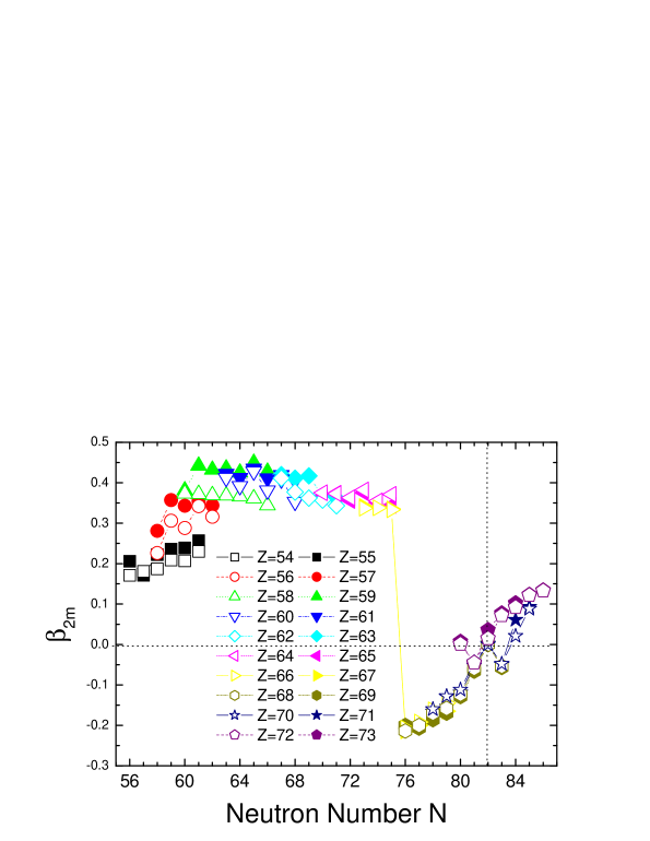
Figure 7: Ground state quadrupole deformations for proton drip-line nuclei with $54\leq Z\leq 73$ as functions of the neutron number, $N$, at and beyond the proton drip line.

For stable even-even nuclei, the information concerning the deformation parameter can be derived from measurements of the $B(E2)\uparrow$ values. The $B(E2)\uparrow$ values are basic experimental quantities that do not depend on the nuclear model. Assuming a uniform charge distribution out to a distance $R(\theta,\phi)$ and zero charge beyond, $\beta_{2p}$ is related to $B(E2)\uparrow$ by

$$\beta_{2p}=(4\pi/3ZR^{2}_{0})[B(E2)\uparrow/e^{2}]^{1/2},$$ (13)

where $R_{0}$ has been taken to be $1.2A^{1/3}$ fm and $B(E2)\uparrow$ is in units of $e^{2}b^{2}$. Unfortunately, we do not have much knowledge about the $B(E2)\uparrow$ values for proton drip-line nuclei. The two available experimental results [52] in the region are $\beta_{2p}=0.221(7)$ for ¹¹⁴Xe and $\beta_{2p}=0.385(48)$ for ¹²⁴Ce, which are in reasonable agreement with our calculations: $\beta_{2p}=0.199$ for ¹¹⁴Xe and $\beta_{2p}=0.344$ for ¹²⁴Ce (also see Fig. 7).

Another source of knowledge for the deformation of proton drip-line nuclei can be obtained from analysis of the properties of proton emitters, as demonstrated in Refs. [4, 5, 6, 7, 8]. In those works, to simplify the calculations the assumption that the parent and daughter nuclei have the same deformation is used. Our calculations show that for Ho, Tm, Lu and Ta isotopes, the parent and daughter nuclei have almost the same deformation. However, for the other six isotopes, an absolute deviation of 0.02–0.09 is found to exist. To what extent such a deviation can influence the conclusions drawn from those calculations [4, 5, 6, 7, 8] needs to be studied in more detail.

4 Conclusion

In the present work, the deformed RMF+BCS model has been used to study the ground state properties of the proton drip-line nuclei with $55\leq Z\leq 73$, including the location of the proton drip line, the ground state quadrupole deformation, the one-proton separation energy, the deformed single-particle orbital occupied by the odd valence proton, and the corresponding spectroscopic factor. The RMF+BCS model reproduces the available experimental data reasonably well, except in the case of odd-odd nuclei. The results also agree well with those of the RHB method. The systematic discrepancies for the one-proton separation energies of the odd-odd proton-rich nuclei may be attributed to the lack of a residual proton-neutron pairing in both mean field models. It will be very interesting to include a residual proton-neutron pairing into the relativistic mean field model through a generalized BCS method in a future work.

In conclusion, we have found that the RMF+BCS model can describe the ground state properties of proton emitters as well as the more complicated RHB model. It is also found that the state-dependent BCS method with a zero-range $\delta$-force is valid not only in the stable region but also in the proton drip line. To summarize, the drip-line nuclei predicted by the RMF+BCS/TMA calculations are ¹⁶¹Ta, ¹⁵⁶Lu, ¹⁵²Tm, ¹⁴⁴Ho, ¹³⁹Tb, ¹³³Eu, ¹²⁹Pm, ¹²⁵Pr, ¹¹⁸La and ¹¹⁵Cs. Based on our calculations, possible proton emitters that could be detected in future experiments are ¹⁴⁹Lu, ¹⁵²Lu, ¹⁵³Lu and ¹⁵⁴Lu for the Lu isotopic chain, ¹⁵⁸Ta for the Ta isotopic chain, ¹³⁰Eu for the Eu isotopic chain, ¹³⁵Tb and ¹³⁶Tb for the Tb isotopic chain, ¹¹⁹Pr and ¹²⁰Pr for the Pr isotopic chain, ¹²⁴Pm and ¹²⁵Pm for the Pm isotopic chain, ¹¹¹Cs for the Cs isotopic chain, and ¹¹⁵La and ¹¹⁶La for the La isotopic chain.

5 Acknowledgments

L. S. Geng is grateful for the Monkasho Fellowship that supported his stay at Research Center for Nuclear Physics, where this work was performed .

References

- [1] P. J. Woods and C. N. Davids, Annu. Rev. Nucl. Part. Sci. 47 (1997), 541.
- [2] S. Aberg, P. B. Semmes and W. Nazarewicz, Phys. Rev. C 56 (1997), 1762.
- [3] M. Notani et al., Phys. Lett. B 542 (2002), 49.
- [4] E. Maglione, L. S. Ferreira and R. J. Liotta, Phys. Rev. Lett. 81 (1998), 538.
- [5] E. Maglione, L. S. Ferreira and R. J. Liotta, Phys. Rev. C 59 (1999), 589(R).
- [6] L. S. Ferreira and E. Maglione, Phys. Rev. C 61 (2000), 021304(R).
- [7] E. Maglione and L. S. Ferreira, Phys. Rev. C 61 (2000), 047307.
- [8] L. S. Ferreira and E. Maglione, Phys. Rev. Lett. 86 (2001), 1721.
- [9] B. D. Serot and J. D. Walecka, Adv. Nucl. Phys. 16 (1986), 1.
- [10] P. G. Reinhard, Rep. Prog. Phys. 52 (1989), 439.
- [11] P. Ring, Prog. Part. Nucl. Phys. 37 (1996), 193.
- [12] D. Hirata, H. Toki, T. Watabe, I. Tanihata and V. Carlson, Phys. Rev. C 44 (1991), 44.
- [13] J. Meng and P. Ring, Phys. Rev. Lett. 77 (1996), 3963.
- [14] J. Meng and P. Ring, Phys. Rev. Lett. 80 (1998), 460.
- [15] J. Meng, Nucl. Phys. A 635 (1998), 3.
- [16] J. Meng, H. Toki, J. Y. Zeng, S. Q. Zhang and S. G. Zhou, Phys. Rev. C 65 (2002), 041302(R).
- [17] H. L. Yadav, S. Sugimoto and H. Toki, Mod. Phys. Lett. A 17 (2002), 2523.
- [18] N. Sandulescu, L. S. Geng, H. Toki and G. C. Hillhouse, Phys. Rev. C 68 (2003), 054323.
- [19] N. Sandulescu, Nguyen Van Giai and R. J. Liotta, Phys. Rev. C 61 (2000), 061301(R).
- [20] L. S. Geng, H. Toki, S. Sugimoto and J. Meng, Prog. Theor. Phys. 110 (2003), 921.
- [21] L. S. Geng, H. Toki, A. Ozawa and J. Meng, Nucl. Phys. A 730 (2004), 80.
- [22] L. S. Geng, H. Toki and J. Meng, Phys. Rev. C 68 (2003), 061303 (R).
-
[23]
Y. Sugahara and H. Toki, Nucl. Phys. A 579 (1994),
557.
Y. Sugahara, Ph.D thesis, Tokyo Metropolitan University, 1995. - [24] G. A. Lalazissis, J. Knig and P. Ring, Phys. Rev C 55 (1997), 540.
- [25] G. A. Lalazissis, D. Vretenar and P. Ring, Phys. Rev. C 60 (1999), 051302(R).
- [26] G. A. Lalazissis, D. Vretenar and P. Ring, Nucl. Phys. A 650 (1999), 133.
- [27] D. Vretenar, G. A. Lalazissis and P. Ring, Phys. Rev. Lett. 82 (1999), 4595.
- [28] G. A. Lalazissis, D. Vretenar and P. Ring, Nucl. Phys. A 679 (2001), 481.
- [29] J. F. Berger, M. Girod and D. Gogny, Nucl. Phys. A 428 (1984), 23c.
- [30] H. Mahmud et al., Phys. Rev. C 64 (2001), 031303(R).
- [31] F. Soramel et al., Phys. Rev. C 63 (2001), 031304(R).
- [32] A. M. Lane, Nuclear Theory (Benjamin, 1964).
- [33] P. Ring and P. Schuck, The Nuclear Many-Body Problem (Springer, 1980).
- [34] H. Flocard et al., Nucl. Phys. A 203 (1973), 433.
- [35] D. Hirata, K. Sumiyoshi, I. Tanihata, Y. Sugahara, T. Tachibana and H. Toki, Nucl. Phys. A 616 (1997), 438c.
- [36] Y. K. Gambhir, P. Ring and A. Thimet, Ann. of Phys. 194 (1990), 132.
- [37] J. Dobaczewski, W. Nazarewicz, T. R. Werner, J. F. Berger, C. R. Chinn and J. Dechargé, Phys. Rev. C 53 (1996), 2809.
- [38] S. Goriely, M. Samyn, P.-H. Heenen, J. M. Pearson and F. Tondeur, Phys. Rev. C 66 (2002), 024326.
- [39] S. Hofmann, Nuclear Decay Modes, D. N. Poenaru and W. Greiner (IOP, Bristol, 1996).
- [40] P. J. Sellin et al., Phys. Rev. C 47 (1993), 1933.
- [41] J. Uusitalo et al., Phys. Rev. C 59 (1999), 2975(R).
- [42] R. D. Page et al., Phys. Rev. Lett. 68 (1992), 1287.
- [43] R. J. Irvine et al., Phys. Rev. C 55 (1997), 1621(R).
- [44] H. T. Chen and A. Goswami, Phys. Lett. B 24 (1967), 257.
- [45] A. L. Goodman, Nucl. Phys. A 186 (1972), 475.
- [46] F. Šimkovic, Ch. C. Moustakidis, L. Pacearescu and Amand Faessler, nucl-th/0308046.
- [47] K. Livingston et al., Phys. Lett. B 312 (1993), 46.
- [48] J. C. Batchelder et al., Phys. Rev. C 57 (1998), 1042(R).
- [49] K. Rykaczewski et al., Phys. Rev. C 60 (1999), 011301(R).
- [50] C. N. Davids et al., Phys. Rev. Lett. 80 (1998), 1849.
- [51] R. D. Page et al., Phys. Rev. Lett. 72 (1994), 1798.
- [52] S. Raman, C. W. Nestor, JR. and P. Tikkanen, At. Data Nucl. Data Tables 78 (2001), 1.