Proton and neutron skins of light nuclei
within the Relativistic Mean Field theory

Abstract

The Relativistic Mean Field (RMF) theory is applied to the analysis of ground-state properties of Ne, Na, Cl and Ar isotopes. In particular, we study the recently established proton skin in Ar isotopes and neutron skin in Na isotopes as a function of the difference between the proton and the neutron separation energy. We use the TMA effective interaction in the RMF Lagrangian, and describe pairing correlation by the density-independent delta-function interaction. We calculate single neutron and proton separation energies, quadrupole deformations, nuclear matter radii and differences between proton radii and neutron radii, and compare these results with the recent experimental data.

, , ,

1 Introduction

One of the most fundamental quantity of the nucleus is its size, nuclear radius, which provides important information on the effect of the nuclear potential, shell effect and ground-state deformation. The presence of neutron skin in stable nuclei has been discussed since the late 1960s [1]. No evidence of appreciable neutron skin in stable nuclei has been observed. A clear evidence has not been obtained even for neutron-rich nuclei until 1990s. During the last decade, developments in accelerator technology and detection techniques [2] have led to an extended study of exotic nuclei near the limits of the $\beta$- stability, especially those light nuclei with $4\leq Z\leq 12$. In particular, measurements of interaction cross sections $(\sigma_{I})$ for light nuclei have been extensively studied at many radioactive nuclear beam facilities and provided important data on nuclear radii [3, 4, 6, 5, 7].

In very neutron-rich nuclei, the weak binding of the outermost neutrons causes the formation of the neutron skin on the surface of a nucleus, and the formation of one- and two-neutron halo structures. Measurements of Na isotopes [3, 4] have revealed a monotonic increase in the neutron skin thickness with increasing neutron number. The established two-neutron halo nuclei are ⁶He, ¹¹Li and ¹⁴Be, and the one-neutron halo nuclei are ¹¹Be and ¹⁹C. Recent data [5] present evidence for a one-neutron halo in ²²N, ²³O and ²³F. On the proton-rich side evidence has been reported for the existence of a proton skin in ²⁰Mg [6]. More recently, Ozawa et al. [7] has confirmed for the first time a monotonic increase of proton skin. These observations indicate that neutron as well as proton skin are quite common phenomena in unstable nuclei far from the stability line. Data on ground-state deformations are also very important for the study of shell effect in exotic nuclei. In particular, they reflect major modifications in the shell structures, the disappearance of traditional and the occurrence of new magic numbers. The new magic number $N=16$ has been reported in the light neutron drip line region [8]. Different ground-state deformations of proton and neutron density distributions are expected in some nuclei with extreme isospin projection quantum number, $T_{z}$.

The Relativistic Mean Field (RMF) theory has been successfully applied to study global properties of nuclei from the proton drip line to the neutron drip line in the entire mass region [9, 10]. The parameter sets, TM1 and TM2, were invented to describe ground-state properties of heavy nuclei ($A>40$; TM1) and light nuclei ($A<40$; TM2) [9]. The parameter set, TM1, has a favorable property of being able to reproduce the essential feature of the equation of state and the vector and the scalar self-energies of the relativistic Bruckner-Hartree-Fock theory for nuclear matter [11]. This parameter set was, however, not able to provide good quantitative results for light nuclei, and the introduction of the other parameter set, TM2, was forced to be made. Considering the RMF Lagrangian with the model parameters as completely a phenomenological model for description of nuclear ground states within the RMF approximation, Sugahara introduced a parameter set smoothly varying with mass and named it as TMA [12], which interpolates the TM1 and the TM2 parameter sets with very week mass dependence. We may interpret this mass dependence as a mean to effectively express the quantum fluctuations beyond the mean field level and/or the softness of the nuclear ground states in deformation, pairing and alpha clustering in light nuclei. On the other side, the parameter set, NL3 [13], is another very successful parameter set for the description of nuclear properties in the entire mass region, which originates from the original non-linear parameter set, NL1 [14]. The NL3 parameter set has removed the unwanted features of NL1 of not being able to obtain stable states for ¹²C and ¹⁶O due to too large attractive contribution of the non-linear terms, while keeping the good properties of the NL1 parameter set for heavy nuclei. It is, therefore, very interesting to compare the theoretical results of the RMF model with these parameter sets, TMA, TM2 and NL3 with the newly obtained systematic data on the light mass region.

In the present work, we apply the recently developed deformed RMF+BCS method with a density-independent delta-function interaction in the pairing channel [15] to the analysis of ground-state properties of Ne, Na, Cl and Ar isotopes. As for the mean field part, we use the TMA, TM2 and the NL3 parameter sets and compare, in particular, the proton and the neutron skins in Ar and Na isotopes. We compare also with the HF+BCS model with the Skyme parameter [16]. We note that there is a work by Lalazissis et al. [17] studying deformed light nuclei, Be, B, C, N, F, Ne and Na isotopes with the Relativistic Hartree-Bogoliubov (RHB) method.

In Sect. 2, we shall present the RMF theory with deformation and pairing correlation. We provide the numerical results in Sect. 3 for Ne, Na, Cl and Ar isotopes. Sect. 4 is devoted to the summery of the present study.

2 Relativistic mean field theory with deformation and pairing

Our RMF calculations have been carried out using the model Lagrangian density with nonlinear terms for both $\sigma$ and $\omega$ mesons as described in detail in Ref. [15], which is given by

$$\begin{array}[]{lll}\mathcal{L}&=&\bar{\psi}(i\gamma^{\mu}\partial_{\mu}-M)\psi+\,\frac{\displaystyle 1}{\displaystyle 2}\partial_{\mu}\sigma\partial^{\mu}\sigma-\frac{\displaystyle 1}{\displaystyle 2}m_{\sigma}^{2}\sigma^{2}-\frac{\displaystyle 1}{\displaystyle 3}g_{2}\sigma^{3}-\frac{\displaystyle 1}{\displaystyle 4}g_{3}\sigma^{4}-g_{\sigma}\bar{\psi}\sigma\psi\\ &&-\frac{\displaystyle 1}{\displaystyle 4}\Omega_{\mu\nu}\Omega^{\mu\nu}+\frac{\displaystyle 1}{\displaystyle 2}m_{\omega}^{2}\omega_{\mu}\omega^{\mu}+\frac{\displaystyle 1}{\displaystyle 4}g_{4}(\omega_{\mu}\omega^{\mu})^{2}-g_{\omega}\bar{\psi}\gamma^{\mu}\psi\omega_{\mu}\\ &&-\frac{\displaystyle 1}{\displaystyle 4}{R^{a}}_{\mu\nu}{R^{a}}^{\mu\nu}+\frac{\displaystyle 1}{\displaystyle 2}m_{\rho}^{2}\rho^{a}_{\mu}\rho^{a\mu}-g_{\rho}\bar{\psi}\gamma_{\mu}\tau^{a}\psi\rho^{\mu a}\\ &&-\frac{\displaystyle 1}{\displaystyle 4}F_{\mu\nu}F^{\mu\nu}-e\bar{\psi}\gamma_{\mu}\frac{\displaystyle 1-\tau_{3}}{\displaystyle 2}A^{\mu}\psi,\\ \end{array}$$ (1)

where the field tensors of the vector mesons and of the electromagnetic field take the following forms:

$$\left\{\begin{array}[]{rl}\Omega_{\mu\nu}=&\partial_{\mu}\omega_{\nu}-\partial_{\nu}\omega_{\mu}\\ R^{a}_{\mu\nu}=&\partial_{\mu}\rho^{a}_{\nu}-\partial_{\nu}\rho^{a}_{\mu}-2g_{\rho}\epsilon^{abc}\rho^{b}_{\mu}\rho^{c}_{\nu}\\ F_{\mu\nu}=&\partial_{\mu}A_{\nu}-\partial_{\nu}A_{\mu}\end{array}\right.$$ (2)

and other symbols have their usual meanings. Based on the single-particle spectrum calculated by the RMF method described above, we perform a state-dependent BCS calculation [18, 19]. The gap equation has a standard form for all the single particle states. i.e.

$$\Delta_{k}=-\frac{\displaystyle 1}{\displaystyle 2}\sum_{k^{\prime}>0}\frac{\displaystyle\bar{V}_{kk^{\prime}}\Delta_{k^{\prime}}}{\displaystyle\sqrt{(\varepsilon_{k^{\prime}}-\lambda)^{2}+\Delta_{k^{\prime}}^{2}}},$$ (3)

where $\varepsilon_{k^{\prime}}$ is the single particle energy and $\lambda$ is the Fermi energy. The particle number condition is given by $2\sum\limits_{k>0}v_{k}^{2}=N$. In the present work we use for the pairing interaction a delta-function interaction, i.e.

$$V=-V_{0}\delta({\bf r_{1}}-{\bf r_{2}}),$$ (4)

with the same strength $V_{0}$ for both protons and neutrons. The pairing matrix element for the delta-function interaction is given by

$$\begin{array}[]{lll}\bar{V}_{ij}&=&\langle i\bar{i}|V|j\bar{j}\rangle-\langle i\bar{i}|V|\bar{j}j\rangle=-V_{0}\int d^{3}r\,\left[\psi^{\dagger}_{i}\psi^{\dagger}_{\bar{i}}\psi_{j}\psi_{\bar{j}}-\psi^{\dagger}_{i}\psi^{\dagger}_{\bar{i}}\psi_{\bar{j}}\psi_{j}\right]\\ \end{array}$$ (5)

with nucleon wave function in the form

$$\psi_{i}({\bf r},t)=\left(\begin{array}[]{c}f_{i}({\bf r})\\ ig_{i}({\bf r})\end{array}\right)=\frac{\displaystyle 1}{\displaystyle\sqrt{2\pi}}\left(\begin{array}[]{l}f^{+}_{i}(z,r_{\bot})e^{i(\Omega_{i}-1/2)\varphi}\\ f^{-}_{i}(z,r_{\bot})e^{i(\Omega_{i}+1/2)\varphi}\\ ig^{+}_{i}(z,r_{\bot})e^{i(\Omega_{i}-1/2)\varphi}\\ ig^{-}_{i}(z,r_{\bot})e^{i(\Omega_{i}+1/2)\varphi}\end{array}\right)\chi_{t_{i}}(t).$$ (6)

A detailed description of the deformed RMF+BCS method can be found in Ref. [15].

In the present study, nuclei with both even and odd number of protons (neutrons) need to be calculated. We adopt a simple blocking method without breaking the time reversal symmetry. The ground state of an odd system is described by the wave function,

$$\alpha^{\dagger}_{k_{1}}|BCS>=\alpha^{\dagger}_{k_{1}}\prod_{k\neq k_{1}}(u_{k}+v_{k}\alpha^{\dagger}_{k}\alpha^{\dagger}_{\bar{k}})|vac>.$$ (7)

Here, $|vac>$ denotes the vacuum state. The unpaired particle sits in the level $k_{1}$ and blocks this level. The Pauli principle prevents this level from participating in the scattering process of nucleons caused by the pairing correlations. As described in Ref. [19], in the calculation of the gap, one level is ”blocked”:

$$\Delta_{k}=-\frac{\displaystyle 1}{\displaystyle 2}\sum_{k^{\prime}\neq k_{1}>0}\frac{\displaystyle\bar{V}_{kk^{\prime}}\Delta_{k^{\prime}}}{\displaystyle\sqrt{(\varepsilon_{k^{\prime}}-\lambda)^{2}+\Delta_{k^{\prime}}^{2}}}.$$ (8)

The level $k_{1}$ has to be excluded from the sum because it can not contribute to the pairing energy. The corresponding chemical potential is determined by

$$N=1+2\sum_{k\neq k_{1}>0}v^{2}_{k}.$$ (9)

The blocking procedure is performed at each step of the self-consistent iteration.

3 Ground state properties of light nuclei

In the present work we take the mass-dependent parameter set TMA [9] for the RMF Lagrangian. Calculations with parameter set TM2 [9] and NL3 [13] are also performed for comparison. In the pairing channel, pairing strength $V_{0}=343.7$ Mev fm³ [15] is taken for both protons and neutrons in the density-independent delta-function interaction. For each nucleus, first the constrained quadrupole calculation [20] is done to obtain all possible ground-state configurations; second we perform the non-constrained calculation using the quadrupole deformation parameter of the deepest minimum of the energy curve of each nucleus as the deformation parameter for our Harmonic Oscillator basis. In the case of several similar minima from the constrained calculation, we repeat the above procedure to botain the configuration with the lowest energy as our final result. The calculations for the present analysis have been carried out by an expansion in 14 oscillator shells for both fermion fields and boson fields. Convergence has been checked with more shells. Following Ref. [21], we fix $\hbar\omega_{0}=41A^{-1/3}$ for fermions. In what follows we discuss the details of our calculations and the numerical results.

3.1 Single neutron and proton separation energy

Single neutron separation energy:

$$S_{n}(Z,N)=B(Z,N)-B(Z,N-1)$$ (10)

and single proton separation energy:

$$S_{p}(Z,N)=B(Z,N)-B(Z-1,N)$$ (11)

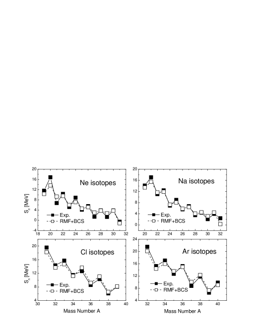
Figure 1: The single neutron separation energis, S_n, of Ne, Na, Cl and Ar isotopes. Results obtained from the deformed RMF+BCS calculations with TMA set are compared with available experimental data [22].

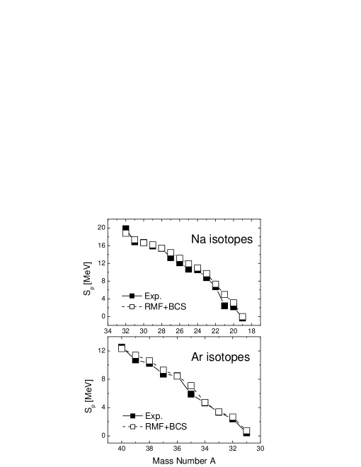
Figure 2: The single proton separation energies, S_p, of Na and Ar isotopes. Results obtained from the deformed RMF+BCS calculations with TMA set are compared with available experimental data [22].

are very important and sensitive quantities of nuclei, where $B(Z,N)$ are the binding energies of nuclei with proton number $Z$ and neutron number $N$. We plot the single neutron separation energies of our calculations with TMA set (empty square) for Ne, Na, Cl and Ar isotopes, together with the available experimental values [22] (solid square) in Fig. 1. Good agreement between experiment and our calculations can be clearly seen. Calculations with TM2 set and NL3 set give practically the same results. For Ne isotopes, our calculations give relative small odd-even staggering than experiment except for ³¹Ne. The most neutron-rich isotope ever observed for Ne isotopes is ³⁴Ne [23] and for Na isotopes it is ³⁷Na [23] , which are consistent with our present calculations (see also Table. 1 and Table. 2). The single proton separation energies of our calculations with TMA set (empty square) for Na and Ar isotopes, together with the available experimental values [22] (solid square) are plotted in Fig. 2. Once again, good agreement between experiment and our calculations can be clearly seen. For ²¹Na, the difference between experiment and our calculations seems somewhat large. We should note that, from the definition of $S_{p}$ (Eq. 11), the single proton separation energy for ²¹Na is related to the binding energies of ²¹Na and ²⁰Ne. While in our calculations the calculated binding energy for ²⁰Ne is about 1.3 MeV smaller than experiment and for ²¹Na is about 1.2 MeV larger than experiment. Thus a total difference of 2.5 MeV is given to the single proton separation energy for ²¹Na. For ³⁵Ar, the relatively large difference comes from the fact that the calculated binding energy for ³⁴Cl is about 2.5 MeV larger than experiment, while calculated binding energy for ³⁵Ar is about 1 MeV larger than experiment. The last bound proton-rich isotope in Na isotopes is predicted to be ²⁰Na in our calculations, which has a single proton separation energy 3.099 MeV. Its one neutron less neighbor, ¹⁹Na, has almost a zero single proton separation energy -0.013 MeV (see also Table. 1 and Table.2). The last bound proton-rich isotope in Ar isotopes is predicted to be ³¹Ar in our calculations, whose $S_{p}$ is 0.741 MeV (see also Table. 3 and Table. 4). All these predictions are consistent with available experimental knowledge [24].

In conclusion, our calculations give a very good description of single neutron and proton separation energies for Ne, Na, Cl and Ar isotopes. All three calculations with different parameter sets, TMA, TM2 and NL3, give essentially the same results. Therefore, we can conclude that the binding energies and single neutron (proton) separation energies are reproduced very well with TMA and NL3 parameter sets, which have been checked by many observables in the entire mass region.

3.2 Root mean square nuclear radius

The root mean square neutron, proton, and matter radii are other important basic physical quantities for nuclei in addition to the single neutron (proton) separation energies. In the RMF theory, the root mean square (rms) neutron, proton and matter radii can be directly deduced from the neutron, proton and matter density distributions, $\rho_{n}$, $\rho_{p}$ and $\rho_{m}$,

$$R_{i}=\langle r^{2}_{i}\rangle^{1/2}=\{\frac{\int\rho_{i}r^{2}d{\bf r}}{\int\rho_{i}d{\bf r}}\}^{1/2},$$ (12)

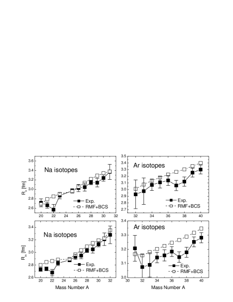
Figure 3: The rms neutron radii, $R_{n}$, and rms matter radii, $R_{m}$, of Na and Ar isotopes. Results obtained from the deformed RMF+BCS calculations with TMA set are compared with available experimental data [3, 4, 7].

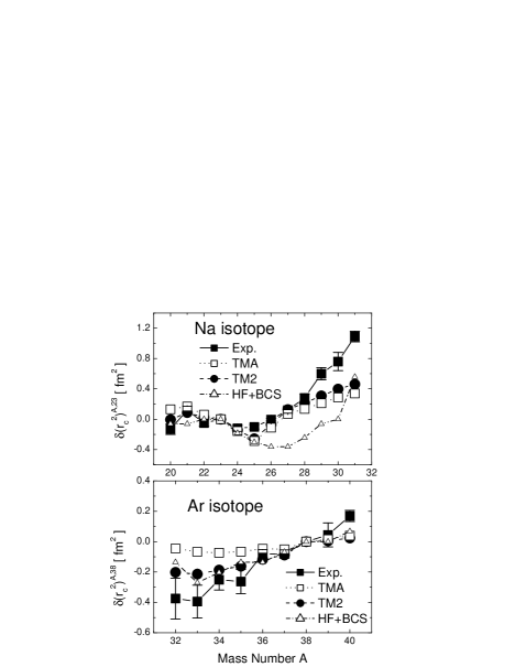
Figure 4: The charge isotope shifts of Na and Ar isotopes. Results obtained from the deformed RMF+BCS calculations with TMA set and TM2 set are compared with available experimental data [26, 27] and results of HF+BCS model [16].

where the index $i\mbox{ }(=n,p,m)$ denotes the corresponding neutron, proton and matter density distributions. First let us have a look at the rms neutron and rms matter radii of Na and Ar isotopes. In Fig. 3, we plot results of our calculations with TMA set and the available experimental values for Na [3, 4] and Ar isotopes [7]. For neutron radii and matter radii of Na isotopes, we notice that our calculations agree very well with experiment except for ²²Na, which has recently been attributed to an admixture of the isomeric state in the beam [4]. For Ar isotopes, although the mass dependence of the experimental data are reproduced quite well, some discrepancies remain. First, the theoretical predictions are at the upper limits of experimental values. Calculations with TM2 set and NL3 set are not better either. Second, the larger radii of $Z=N$ nuclei ³⁶Ar than those of its neighbors has been interpreted to be a possible alpha-cluster structure [25]. Third, our calculations do not reproduce the abrupt decrease of ³⁷Ar and ³⁸Ar. The relatively larger radii of proton drip line nucleus ³¹Ar can be understood easily if we note that ³¹Ar is the last bound proton-rich isotope in Ar isotopes. Second we plot the charge isotope shifts of our calculations with TMA set (empty square) together with the experimental values (solid square) for Na isotopes [26] and Ar isotopes [27] in Fig. 4. Calculations with TM2 set (solid circle) and results of HF+BCS model [16] are also shown for comparison. For Na isotopes, significant difference between the theoretical predictions and the experimental values exist in two regions. The first is ²⁵Na, and the second is around the region of neutron drip line $A\geq 29$. While for Ar isotopes, calculations with TM2 set agree very well with the experimental values within the error bar except for ⁴⁰Ar. For both isotopes, results with TM2 set are closer to the experimental values. It is not surprising because TM2 is a parameter set specially made for light nuclei. For further comparison with other theories, we include the results of the HF+BCS model [16] in Fig. 4. As for Ne isotopes, the isotope shifts start to deviate from ²⁶Ne to the lower side except for ³¹Ne. On the other hand, the results for Ar isotopes agree very well with experiment and are similar to those of the RMF+BCS with TM2 parameter set except for ³²Ar.

To conclude, the deformed RMF+BCS method describe the rms neutron radii and matter radii very well. While for rms charge (proton) radii, although the basic trend is reproduced quite well, the results are not so satisfactory considering that we obtain the parameter set by fitting the charge radii of certain nuclei. However, we might have to pay more attention to the various cluster phenomena, which make it difficult to apply the mean field theory to light nuclei.

3.3 Neutron skin and proton skin

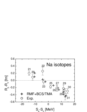
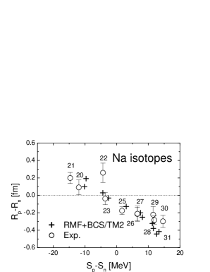
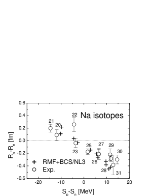
Figure 5: The proton skins, $R_{p}-R_{n}$, plotted as functions of the difference between the proton and neutron separation energy, $S_{p}-S_{n}$. We show the theoretical results with all the three parameter sets, TMA, TM2 and NL3, from top to bottom. The corresponding experimental data are taken from Ref. [3, 4, 7, 22].

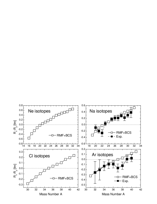
Figure 6: The neutron skins, $R_{n}-R_{p}$, of Ne, Na, Cl and Ar isotopes. Results obtained from the deformed RMF+BCS calculations with TMA set are compared with available experimental data [3, 4, 7].

Different theories, both relativistic and non-relativistic ones, have predicted the existence of proton skin and neutron skin since long time ago, but only recently experimental physicists have proved the theoretical predictions. In Fig. 5, the proton skin $\Delta R=R_{p}-R_{n}$ is plotted against the difference between the proton and neutron separation energy $\Delta S=S_{p}-S_{n}$. It can be clearly seen that $\Delta R$ has a strong correlation with $\Delta S$. Thus, it is shown that the difference between the proton and neutron Fermi energy is the driving force for the creation of the skin phenomenon. Such a correlation has already been predicted by RMF theory since a decade ago [28]. For Na isotopes, calculations with NL3 set predict smaller $\Delta S$ for ^28-31Na, while calculations with TMA and TM2 sets are in better agreement with experimental $\Delta S$ values. For Ar isotopes, all three calculations failed to reproduce the experimental observed proton-skin in ³⁷Ar and ³⁸Ar. In Fig. 6, we plot neutron skin $R_{n}-R_{p}$ against mass number A for Ne, Na, Cl and Ar isotopes. From Figure. 6, it is quite clear that neutron (proton) skin are quite common for neutron-rich (proton-rich) nuclei.

In the Relativistic Mean Field theory, the formation of skin or halo is usually explained by the picture of a core plus a few occupied loosely bound (unbound) states of small angular momentum. The halo in ¹¹Li has been successfully reproduced in this picture [29] where the occupations of 1p_1/2 and 2s_1/2 state are found to be important. Based on the similar picture, giant-halos in ^124-138Zr have been predicted by both RCHB [30] method and resonant RMF-rBCS method [31]. In Ref. [31], it has been shown that 3p_3/2, 2f_7/2 and 3p_1/2 states contribute most to the formation of halo in ¹²⁴Zr. In order to reproduce the sudden increase of rms neutron (proton) radii, which is one indication of halo structure, the Relativistic Mean Field model must be solved in coordinate space. Although, compared with RCHB method, quite similar two neutron separation energies are obtained in the deformed RMF+BCS method [15], the sudden increase of rms neutron radii for ^124-138Zr are not reproduced well. Some improvements on the expansion method could improve the tail behavior of resonant wave functions and solve this problem finally. Possible candidates are the expansion method in the local transformed Harmonic Oscillator basis [32] and the expansion method in a Woods-Saxon basis [33]. This work is under way now. However, as we can see from our calculations, such a disadvantage of Harmonic Oscillator basis does not influence our conclusions here.

3.4 Deformation parameter

Compared with binding energies and nuclear radii, predicted deformation parameters of nuclei are quite different from model to model. One reason is, of course, the possible shape coexistence. Another reason is that deformation parameters are more sensitive to model details. On the experimental side, we can obtain the information of nuclear deformation from measurements of $B(E2)\uparrow$ values. The $B(E2)\uparrow$ values are basic experimental quantities that do not depend on nuclear models. Assuming a uniform charge distribution out to the distance $R(\theta,\phi)$ and zero charge beyond, $\beta_{2p}$ [34, 15] is related to $B(E2)\uparrow$ by

$$\beta_{2p}=(4\pi/3ZR^{2}_{0})[B(E2)\uparrow/e^{2}]^{1/2},$$ (13)

where $R_{0}$ has been taken to be $1.2A^{1/3}$ fm and $B(E2)\uparrow$ is in units of $e^{2}b^{2}$. $B(E2)\uparrow$ values have been measured mainly for some even-even nuclei.

In Fig. 7, we plot the deformation parameter $\beta_{2p(m)}$ for Ne, Na, Cl and Ar isotopes against mass number A. For our RMF+BCS calculations, we plot $\beta_{2p}$ because as we can see from Eq. (13) that what we obtain from $B(E2)\uparrow$ is actually $\beta_{2p}$, not $\beta_{2m}$. For the Finite Range Droplet Model (FRDM) [35], the plotted deformation parameter is $\beta_{2m}$. Except for exotic nuclei with extreme N/Z ratios, we note that these two values are very close to each other (see also Table. 1 $\sim$ 4). From Fig. 7, we see that experimental values show that Ne isotopes are super deformed ($\beta_{2p}\approx 0.6$) in the region $A=18\sim 28$. Except for ²⁰Ne and ²²Ne, our calculations failed to reproduce ¹⁸Ne, ²⁴Ne, ²⁶Ne and ²⁸Ne. For Na isotopes, both our calculations and FRDM predict prolate shapes. For Cl isotopes, a transition between prolate shapes and oblate shapes have been predicted by both methods. For Ar isotopes, our calculations predict oblate shapes for most nuclei while FRDM predict spherical shapes. Except for ³⁸Ar, our predictions agree very well with experimental values. We should mention here that, because from the $B(E2)\uparrow$ values, we can not distinguish prolate or oblate shapes, we just put a random sign before the experimental value to make it close to our predictions. This does not change the essence of our comparison.

4 Summary

We have studied light nuclei, in particular, Ne, Na, Cl and Ar isotopes, in the framework of the deformed RMF+BCS method. The deformation is treated by using the expansion method in the deformed Harmonic Oscillator basis. We have used TMA, TM2 and NL3 effective interactions in the RMF Lagrangian. In addition we have treated the pairing correlations in terms of a density-independent delta-function interaction.

We have calculated neutron (proton) separation energies, quadrupole deformations, nuclear neutron (proton) and matter radii. All the results are presented in the form of tables (Table. I $\sim$ IV). We have compared the calculated results with three parameter sets, TMA, TM2 and NL3, with the available experimental values. Both TMA and NL3 parameter sets are often used in the RMF theory in the entire mass region from the proton drip line to the neutron drip line. We have used TM2 parameter set also, which is extracted particularly for light nuclei. All the three parameter sets provide similar results in our present calculations.

The single neutron (proton) separation energies are reproduced very well within the deformed RMF+BCS method with all the three parameter sets. The general trends of the rms neutron radii come out to be also very good. However, the rms proton radii seem to be generally overestimated in the deformed RMF+BCS method in comparison with experimental values. We have extracted also the nuclear deformations by the minimization method. In general, the calculated results are in good agreement with experimental values extracted from the $BE(2)\uparrow$ values. The discrepancy on the proton radii for these light nuclei may be related with the softness of the light nuclei in deformation and in alpha-clustering, which are not included in the mean field Lagrangian. We have to study the effect of the softness in future works

5 Acknowledgments

L.S. Geng is grateful to the Monkasho fellowship for supporting his stay at Research Center for Nuclear Physics where this work is done .

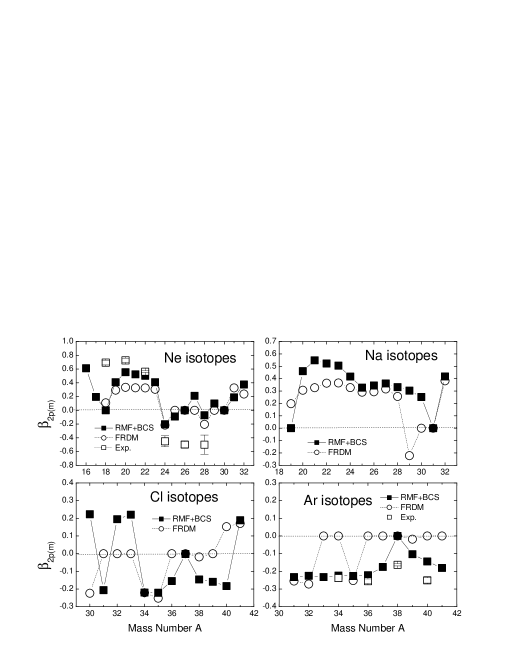
Figure 7: The deformation parameters, $\beta_{2p(m)}$, of Ne, Na, Cl and Ar isotopes. Results obtained from the deformed RMF+BCS calculations with TMA set are compared with available experimental data [34] and results of FDRM model [35].

Table 1: The ground state properties of Ne isotopes ($Z=10$) calculated with the parameter set TMA. Listed are the total binding energy, $B$, the binding energy per nucleon, $B/A$ , charge, neutron, proton, and matter root mean square radii, $R_{c}$, $R_{n}$, $R_{p}$ and $R_{m}$, and the quadrupole deformation parameter for the neutron, proton and matter distributions, $\beta_{2n}$, $\beta_{2p}$ and $\beta_{2m}$, with $A$ the mass number and $N$ the neutron number.

$A$	$N$	$B$	$B/A$	$R_{c}$	$R_{n}$	$R_{p}$	$R_{m}$	$\beta_{2n}$	$\beta_{2p}$	$\beta_{2m}$
16	6	99.115	6.196	3.0845	2.4177	2.9789	2.7818	0.249	0.612	0.476
17	7	116.263	6.839	2.9811	2.4967	2.8717	2.7236	0.076	0.195	0.146
18	8	135.379	7.521	2.9196	2.5598	2.8078	2.7004	0.000	0.000	0.000
19	9	145.724	7.670	2.9194	2.6811	2.8077	2.7485	0.308	0.409	0.361
20	10	159.367	7.968	2.9392	2.8011	2.8282	2.8147	0.541	0.554	0.548
21	11	168.666	8.032	2.9251	2.8604	2.8135	2.8382	0.531	0.523	0.528
22	12	178.234	8.102	2.9176	2.9155	2.8057	2.8661	0.527	0.502	0.515
23	13	184.257	8.011	2.8942	2.9462	2.7814	2.8757	0.375	0.409	0.390
24	14	191.392	7.975	2.8637	2.9726	2.7497	2.8818	-0.235	-0.203	-0.222
25	15	195.991	7.840	2.8672	3.0642	2.7533	2.9438	-0.086	-0.090	-0.088
26	16	201.148	7.736	2.8825	3.1613	2.7693	3.0165	0.000	0.000	0.000
27	17	204.194	7.563	2.9250	3.2443	2.8135	3.0917	0.181	0.210	0.191
28	18	207.988	7.428	2.9392	3.3118	2.8283	3.1476	-0.069	-0.071	-0.070
29	19	210.725	7.266	2.9643	3.3695	2.8543	3.2012	0.071	0.099	0.081
30	20	214.508	7.150	2.9863	3.4206	2.8772	3.2496	0.000	0.000	0.000
31	21	213.381	6.883	3.0102	3.5274	2.9020	3.3385	0.210	0.190	0.203
32	22	215.128	6.723	3.0655	3.6155	2.9593	3.4240	0.388	0.376	0.384
33	23	215.486	6.530	3.0905	3.6820	2.9851	3.4856	0.453	0.407	0.439
34	24	216.331	6.363	3.1159	3.7446	3.0115	3.5447	0.513	0.436	0.491

Table 2: The same as Table 1, but for Na isotopes ($Z=11$).

$A$	$N$	$B$	$B/A$	$R_{c}$	$R_{n}$	$R_{p}$	$R_{m}$	$\beta_{2n}$	$\beta_{2p}$	$\beta_{2m}$
18	7	115.054	6.392	3.0876	2.5260	2.9822	2.8136	0.193	0.503	0.383
19	8	135.366	7.125	2.9995	2.5642	2.8908	2.7580	0.000	0.001	0.001
20	9	148.823	7.441	2.9985	2.6863	2.8899	2.8001	0.325	0.461	0.400
21	10	164.329	7.825	3.0044	2.7928	2.8960	2.8473	0.516	0.549	0.533
22	11	175.991	8.000	2.9865	2.8493	2.8774	2.8634	0.512	0.523	0.517
23	12	187.934	8.171	2.9764	2.9020	2.8668	2.8853	0.511	0.506	0.508
24	13	195.248	8.135	2.9501	2.9297	2.8395	2.8887	0.369	0.417	0.391
25	14	203.333	8.133	2.9279	2.9557	2.8165	2.8953	0.243	0.328	0.280
26	15	209.157	8.044	2.9579	3.0555	2.8477	2.9694	0.288	0.345	0.312
27	16	215.574	7.984	2.9878	3.1383	2.8787	3.0352	0.333	0.362	0.345
28	17	219.644	7.844	2.9992	3.2198	2.8905	3.0946	0.259	0.332	0.288
29	18	224.209	7.731	3.0116	3.2903	2.9034	3.1491	0.198	0.304	0.238
30	19	227.366	7.579	3.0243	3.3416	2.9165	3.1923	0.126	0.252	0.172
31	20	231.868	7.480	3.0330	3.3784	2.9256	3.2250	0.000	0.000	0.000
32	21	232.198	7.256	3.0989	3.5270	2.9938	3.3533	0.433	0.418	0.428
33	22	235.422	7.134	3.1079	3.5611	3.0031	3.3853	0.361	0.371	0.364
34	23	236.869	6.967	3.1330	3.6225	3.0292	3.4418	0.419	0.404	0.414
35	24	238.780	6.822	3.1588	3.6815	3.0558	3.4969	0.476	0.435	0.463
36	25	238.540	6.626	3.1726	3.7808	3.0701	3.5786	0.531	0.434	0.501
37	26	238.831	6.455	3.1840	3.8488	3.0818	3.6377	0.540	0.426	0.506

Table 3: The same as Table 1, but for Cl isotopes ($Z=17$).

$A$	$N$	$B$	$B/A$	$R_{c}$	$R_{n}$	$R_{p}$	$R_{m}$	$\beta_{2n}$	$\beta_{2p}$	$\beta_{2m}$
28	11	187.833	6.708	3.4060	2.8804	3.3107	3.1487	0.336	0.271	0.297
29	12	208.281	7.182	3.3718	2.9316	3.2755	3.1378	0.352	0.287	0.314
30	13	225.271	7.509	3.3264	2.9484	3.2287	3.1104	0.233	0.223	0.227
31	14	243.494	7.855	3.3031	2.9843	3.2048	3.1072	-0.193	-0.206	-0.200
32	15	257.174	8.037	3.2968	3.0439	3.1983	3.1269	0.198	0.195	0.196
33	16	271.847	8.238	3.3053	3.1084	3.2070	3.1596	0.250	0.221	0.235
34	17	283.061	8.325	3.3055	3.1699	3.2073	3.1886	-0.204	-0.220	-0.212
35	18	296.711	8.477	3.3140	3.2188	3.2160	3.2174	-0.218	-0.221	-0.220
36	19	305.930	8.498	3.3145	3.2574	3.2165	3.2382	-0.117	-0.155	-0.135
37	20	316.981	8.567	3.3211	3.2986	3.2233	3.2642	-0.001	-0.002	-0.002
38	21	323.520	8.514	3.3255	3.3515	3.2278	3.2968	-0.102	-0.146	-0.122
39	22	331.685	8.505	3.3328	3.4005	3.2354	3.3295	-0.126	-0.159	-0.140
40	23	337.720	8.443	3.3433	3.4420	3.2462	3.3602	-0.164	-0.183	-0.172
41	24	345.731	8.432	3.3498	3.4892	3.2529	3.3932	0.219	0.189	0.207

Table 4: The same as Table 1, but for Ar isotopes ($Z=18$).

$A$	$N$	$B$	$B/A$	$R_{c}$	$R_{n}$	$R_{p}$	$R_{m}$	$\beta_{2n}$	$\beta_{2p}$	$\beta_{2m}$
29	11	186.450	6.429	3.4869	2.8961	3.3939	3.2142	0.317	0.212	0.252
30	12	207.631	6.921	3.4499	2.9427	3.3559	3.1970	0.325	0.217	0.260
31	13	226.012	7.291	3.3926	2.9750	3.2970	3.1659	-0.208	-0.232	-0.222
32	14	246.157	7.692	3.3631	3.0111	3.2665	3.1573	-0.203	-0.225	-0.215
33	15	260.569	7.896	3.3598	3.0769	3.2631	3.1799	-0.214	-0.232	-0.224
34	16	276.577	8.135	3.3589	3.1345	3.2622	3.2027	-0.207	-0.224	-0.216
35	17	290.163	8.290	3.3600	3.1818	3.2634	3.2240	-0.216	-0.226	-0.221
36	18	305.154	8.477	3.3628	3.2264	3.2662	3.2464	-0.215	-0.222	-0.218
37	19	315.220	8.519	3.3623	3.2663	3.2657	3.26660	-0.217	-0.175	-0.151
38	20	327.581	8.621	3.3698	3.3038	3.2735	3.2895	0.000	0.000	0.000
39	21	334.913	8.588	3.3722	3.3521	3.2759	3.3171	-0.085	-0.103	-0.093
40	22	344.011	8.600	3.3756	3.4003	3.2795	3.3464	-0.115	-0.144	-0.128
41	23	351.032	8.562	3.3830	3.4418	3.2870	3.3747	-0.159	-0.181	-0.168

References

- [1] W.D. Myers and W.J. Swiatecki, Ann. Phys. (N.Y.) 55 (1969) 395
- [2] I. Tanihata, Prog. Part. Nucl. Phys. 35 (1995) 505.
- [3] T. Suzuki, et al., Phys. Rev. Lett. 75 (1995) 3241.
- [4] T. Suzuki, et al., Nucl. Phys. A 630 (1998) 661.
- [5] A. Ozawa, et al., Nucl. Phys. A 691 (2001) 599.
- [6] L. Chulkov, et al., Nucl. Phys. A 603 (1996) 219.
- [7] A. Ozawa, et al., Nucl. Phys. A 709 (2002) 60.
- [8] A. Ozawa, T. Kobayashi, T. Suzuki, K. Yoshida and I. Tanihata, Phys. Rev. Lett. 84 (2000) 5493.
- [9] Y. Sugahara and H. Toki, Nucl. Phys. A 579 (1994) 557.
- [10] P. Ring, Prog. Part. Nucl. Phys. 37 (1996) 193.
- [11] R. Brockmann and R. Machleidt, Phys. Rev. C 42 (1990) 1965.
- [12] Y. Sugahara, Doctor thesis in Tokyo Metropolitan University (1995).
- [13] G. A. Lalazissis, J. Knig, and P. Ring, Phys. Rev C 55 (1997) 540.
- [14] P.G. Reinhard, M. Rufa, J. Maruhn, W. Greiner, and J. Friedrich, Z. Phys. A 323 (1986) 13.
- [15] L.S. Geng, H. Toki, S. Sugimoto and J. Meng, Prog. Theor. Phys. 110 (2003), 921.
- [16] S. Goriely, F. Tondeur, J.M. Pearson, At. Data Nucl. Data Tables 77 (2001) 371.
- [17] G.L. Lalazissis, D. Vretenar and P. Ring, arXiv:nucl-th/0109027
- [18] A. M. Lane, Nuclear Theory (Benjamin, 1964).
- [19] P. Ring and P. Schuck, The Nuclear Many-Body Problem (Springer, 1980).
- [20] F. Floard et al., Nucl. Phys. A 203 (1973) 433.
- [21] Y.K. Gambhir, P. Ring and A. Thimet, Ann. Phys. (N.Y.) 194 (1990) 132.
- [22] G. Audi and A. H. Wapstra, Nucl. Phys. A 595 (1995) 409.
- [23] M. Notani et al., Phys. Lett. B 542 (2002) 49.
- [24] P.J. Woods and C.N. Davids, Annu. Rev. Nucl. Part. Sci. 47 (1997) 541.
- [25] A. Ozawa, et al., Nucl. Phys. A 608 (1996) 63.
- [26] E.W. Otten, in Treatise on Heavy-IOn Science, edited by D.A. Bromley (Plenum, New York, 1989) Vol 8, p. 515
- [27] A. Klein et al., Nucl. Phys. A 607 (1996) 1.
- [28] I. Tanihata et al., Phys. Lett. B 289 (1992) 261.
- [29] J. Meng and P. Ring, Phys. Rev. Lett. 77 (1996) 3963; J. Meng, Nucl. Phys. A 635 (1998) 3.
- [30] J. Meng and P. Ring, Phys. Rev. Let. 80 (1998) 460.
- [31] N. Sandulescu, L.S. Geng, H. Toki, and G. Hillhouse, arXiv:nucl-th/0306035.
- [32] M.V. Stoitsov, W. Nazarewicz and S. Pittel, Phys. Rev. C 58 (1998) 2092.
- [33] S.G. Zhou, J. Meng and P. Ring, Phys. Rev. C 68 (2003) 034323.
- [34] S. Raman, C.W. Nestor, JR., and P. Tikkanen, At. Data Nucl. Data Tables 78 (2001) 1.
- [35] P. Möller, J. R. Nix, W.D. Myers, and W.J. Swiatecki, At Data Nucl. Data Tables 59 (1995) 185.