Two-neutrino double beta decay within Fully-Renormalized QRPA: Effect of the restoration of the Ikeda sum rule

Abstract

The recently proposed Fully-Renormalized QRPA (FR-QRPA), which fullfils the Ikeda sum rule (ISR) exactly, is applied to the two-neutrino double beta decay of ⁷⁶Ge, ⁸²Se, ¹⁰⁰Mo, ¹¹⁶Cd, ¹²⁸Te and ¹³⁰Xe. The results obtained are compared with those of other approaches, standard QRPA and self-consistent QRPA (SCQRPA). The similarities and the differences among the methods are discussed. The influence of the restoration of the Ikeda sum rule on the $2\nu\beta\beta$-decay amplitude is analyzed.

I Introduction

Observation of the neutrinoless double beta decay ($0\nu\beta\beta$-decay), violating the total lepton number by two units, would give unambiguous evidence for new physics beyond the Standard Model [1, 2, 3]. For instance, at least one of the neutrinos would have to be a Majorana particle with non-zero mass [4]. The current experimental upper limits on the $0\nu\beta\beta$-decay half-life impose stringent constraints, e.g., on the parameters of Grand Unification and super-symmetric extensions of the Standard Model.

Rates of the $2\nu\beta\beta$-decay, which is a second order process allowed within the Standard Model, can be calculated within the same nuclear structure models. Thus, the results of the nuclear structure calculations can be directly compared with the corresponding experimental data available for a number of nuclei [6]. Such a comparison provides a very useful test of the models.

The Quasiparticle Random Phase Approximation (QRPA) [5] has been successfully exploited in nuclear physics to describe properties of the excited states of open-shell nuclei and to calculate intensities of various nuclear reactions, including the double beta decay (see reviews [1]).

It was shown that the experimental data on the $2\nu\beta\beta$-decay rates can be reproduced in QRPA calculations with a sufficiently large strength of the particle-particle interaction [7]. But the proximity of the value to the point of the QRPA collapse questions the reliability of the results. It is known that QRPA collapse occurs due to the use of the quasi-boson approximation (QBA) which violates the Pauli exclusion principle (PEP) and generates too many ground state correlations.

Renormalized QRPA (RQRPA) was formulated in Refs. [8] to restore PEP in an approximate way. The main goal of the method is to use a self-consistent iteration of the QRPA equation with taking into account quasiparticle occupation numbers in the QRPA ground state. That leads to a modification of the commutation relations for bifermionic operators as compared to the ordinary quasiboson approximation (QBA). At the same time so-called scattering terms (describing transitions of the quasiparticles) are neglected in the Hamiltonian and in the phonon operators. The RQRPA does not collapse for physical values of the particle-particle interaction strength and has been extensively used to calculate the intensities of the double beta decay [1, 10, 11]. It has been also shown that the RQRPA provides better agreement with the exact solution of the many-body problem within schematic models, even beyond the critical point of the standard QRPA (see, e.g. [9] and references therein).

The self-consistent RQRPA (SCQRPA) is a more complex version of RQRPA to describe the strongly correlated Fermi systems. Within this method one goes a step further beyond the RQRPA. In the SCQRPA at the same time the quasiparticle mean field is changed by minimizing the energy and fixing the number of particles in the correlated ground state of RQRPA instead of the uncorrelated one of BCS as is done in the other versions of the RQRPA. In this way SCQRPA partially overcomes the inconsistency between RQRPA and the BCS approach and is closer to a fully variational theory.

Nevertheless, the main drawback of the modern versions of RQRPA and SCQRPA is the violation of the model-independent Ikeda sum rule (ISR) [11, 12, 13]. A modification of the phonon operator by including scattering terms is needed in order to restore the ISR within RQRPA. The fully-Renormalized QRPA (FR-QRPA) was formulated in Ref. [16] for even-even nuclei in such a way that it complies with restrictions imposed by the commutativity of the phonon creation operator with the total particle number operator. It was shown analytically that the Ikeda sum rule is fulfilled within the FR-QRPA [16]. Also FR-QRPA is free from the spurious low-energy solutions which would be generated by the scattering terms considered as additional degrees of freedom as suggested in [17].

The aim of the paper is twofold. First, we would like to describe the FR-QRPA equations in more details (as compared with the original paper [16]) for a simple case of a Hamiltonian with the separable residual interaction in both particle-hole and particle-particle channels. Second, the first numerical application of FR-QRPA is given to calculate $2\nu\beta\beta$-decay intensities and relevant quantities. So far, the full convergence of the FR-QRPA solution has been obtained only for a rather small model space. Nevertheless a comparison of the results obtained within FR-QRPA and SCQRPA can be provided.

II Basic relationships of the Fully-Renormalized QRPA

Within RPA an excited nuclear state, with angular momentum $J$ and projection $M$, is created by applying the phonon operator $Q^{\dagger}_{JM}$ to the vacuum state $|0^{+}_{RPA}\rangle$ of the initial, even-even, nucleus:

$$|JM\rangle=Q^{\dagger}_{JM}|0^{+}_{RPA}\rangle\qquad\mbox{with}\qquad Q_{JM}|0^{+}_{RPA}\rangle=0.$$ (1)

As was shown in Ref. [16], the most appropriate way is to write down the phonon structure in terms of the particle creation and annihilation operators. That allows to fulfill the important principle of the commutativity of $Q^{\dagger}_{JM}$ with the total particle number operator $\hat{A}=\hat{N}+\hat{Z}$. The phonon operator has the following structure:

$$Q^{\dagger}_{JM}=\sum\limits_{pn}\left[x_{(pn,J)}C^{\dagger}(pn,JM)-y_{(pn,J)}\tilde{C}(pn,JM)\right],$$ (2)

with $C^{\dagger}(pn,JM)=\left[c^{\dagger}_{p}{\tilde{c}}_{n}\right]_{JM}$ and $\tilde{C}(pn,JM)=(-)^{J-M}C(pn,J\,-M)$, where $c^{+}_{\tau m_{\tau}}$ ($c_{\tau m_{\tau}}$) denotes the particle creation (annihilation) operator for protons and neutrons ($\tau=p,n$).

Going into the quasiparticle representation, the quasiparticle creation and annihilation operators $a^{+}_{\tau m_{\tau}}$ and $a_{\tau m_{\tau}},(\tau=p,n)$ can be defined by the Bogolyubov transformation

$$\left(\matrix{a^{+}_{\tau m_{\tau}}\cr{\tilde{a}}_{\tau m_{\tau}}}\right)=\left(\matrix{u_{\tau}&v_{\tau}\cr-v_{\tau}&u_{\tau}}\right)\left(\matrix{c^{+}_{\tau m_{\tau}}\cr{\tilde{c}}_{\tau m_{\tau}}}\right),$$ (3)

that leads to the following expression for the phonon operator $Q^{\dagger}_{JM}$:

$$Q^{\dagger}_{JM}=\sum\limits_{{p}{n}}\left[X_{({p}{n},J)}\bar{A}^{\dagger}({p}{n},JM)-Y_{({p}{n},J)}\tilde{\bar{A}\,}({p}{n},JM)\right],$$ (4)

(5)

$$\bar{A}^{\dagger}=A^{\dagger}+\left(u_{n}v_{n}B^{\dagger}-u_{p}v_{p}\tilde{B}\right)\left/(v_{n}^{2}-v_{p}^{2})\right.$$ (6)

$$A^{\dagger}(pn,JM)=\left[a^{\dagger}_{p}a^{\dagger}_{n}\right]_{JM}\ ;\ \ B^{\dagger}(pn,JM)=\left[a^{\dagger}_{p}{\tilde{a}}_{n}\right]_{JM}$$ (7)

where $X=u_{p}v_{n}x-v_{p}u_{n}y,\ Y=u_{p}v_{n}y-v_{p}u_{n}x$. The bifermionic operators $\bar{A}^{\dagger},\bar{A}$ now being the basic building blocks of the FR-QRPA automatically contain the quasiparticle scattering terms which, however, are not associated with any additional degree of freedom. That means that there are no spurious low-lying solutions in the present theoretical scheme which would be generated by the scattering terms considered as independent constituents of the phonon operator (as proposed in [17]).

From this point we can follow the usual way to formulate the RQRPA [8], substituting $A$ by $\bar{A}$ everywhere. The forward- and backward-going free variational amplitudes X and Y satisfy the equation:

$$\left(\begin{array}[]{cc}{\cal A}&{\cal B}\\ {\cal B}&{\cal A}\end{array}\right)\left(\begin{array}[]{c}X^{m}\\ Y^{m}\end{array}\right)={\cal E}_{m}\left(\begin{array}[]{cc}{\cal U}&0\\ 0&{\cal-U}\end{array}\right)\left(\begin{array}[]{c}X^{m}\\ Y^{m}\end{array}\right),$$ (8)

where $m$ marks different roots of the QRPA equations for a given $J^{\pi}$,

$${\cal A} = \langle 0^{+}_{RPA}|\left[\bar{A},\left[H,\bar{A}^{\dagger}\right]\right]|0^{+}_{RPA}\rangle,$$ (9)

$${\cal B} = -\langle 0^{+}_{RPA}|\left[\bar{A},\left[H,\bar{A}\right]\right]|0^{+}_{RPA}\rangle,$$ (10)

and the renormalization matrix ${\cal U}_{pn}$ is

$${\cal U}_{pn} = \langle 0^{+}_{RPA}|\left[\bar{A}(pn,JM),\bar{A}^{\dagger}(p^{\prime}n^{\prime},JM)\right]|0^{+}_{RPA}\rangle=\delta_{pp^{\prime}}\delta_{nn^{\prime}}{\cal D}_{pn}.$$ (11)

We use a rather simple, but realistic, Hamiltonian $H$ consisting of the quasiparticle mean field $H_{0}$ and the residual separable particle–hole (ph) and particle–particle (pp) interactions:

$$H=H_{0}+H^{ph}_{int}+H^{pp}_{int},$$ (12)

$$H_{0}=\sum\limits_{\tau=p,n}E_{\tau}a^{\dagger}_{\tau}a_{\tau},$$ (13)

$$H_{int}^{ph}=~{}\chi\sum\limits_{M}(-1)^{M}(\beta^{-}_{1M}\beta^{+}_{1-M}+\beta^{+}_{1-M}\beta^{-}_{1M}),$$ (14)

$$H_{int}^{pp}=-\kappa\sum\limits_{M}(-1)^{M}(P^{-}_{1M}P^{+}_{1-M}+P^{+}_{1-M}P^{-}_{1M}),$$ (15)

with $\beta_{1M}^{-}=-\hat{J}^{-1}\sum\limits_{pn}\langle p\|\sigma\|n\rangle\left[c^{\dagger}_{p}{\tilde{c}}_{n}\right]_{1M}$, $P_{1M}^{-}=\hat{J}^{-1}\sum\limits_{pn}\langle p\|\sigma\|n\rangle\left[c^{\dagger}_{p}c^{\dagger}_{n}\right]_{1M}$ and $J=1$.

Taking into account the exact (fermionic) expressions for the commutators in (10),(11), one gets the following expressions for the FR-QRPA matrices ${\cal A}$ and ${\cal B}$:

$${\cal A} = \left[(E_{p}+E_{n}){\cal D}_{pn}-2(E_{p}-E_{n})(u_{p}^{2}v_{p}^{2}+u_{n}^{2}v_{n}^{2}){\cal R}_{pn}\right]\delta_{pp^{\prime}}\delta_{nn^{\prime}}$$ (18)

$$+2\chi(u_{p}v_{n}u_{p^{\prime}}v_{n^{\prime}}+v_{p}u_{n}v_{p^{\prime}}u_{n^{\prime}}){\cal D}_{pn}{\cal D}_{p^{\prime}n^{\prime}}$$

$$-2\kappa(u_{p}u_{n}u_{p^{\prime}}u_{n^{\prime}}{\bar{\bar{\cal D}}}_{pn}{\bar{\bar{\cal D}}}_{p^{\prime}n^{\prime}}+v_{p}v_{n}v_{p^{\prime}}v_{n^{\prime}}{\bar{\cal D}}_{pn}{\bar{\cal D}}_{p^{\prime}n^{\prime}}),$$

$${\cal B} = 2(E_{p}-E_{n})u_{p}v_{p}u_{n}v_{n}{\cal R}_{pn}\delta_{pp^{\prime}}\delta_{nn^{\prime}}$$ (22)

$$+2\chi(u_{p}v_{n}v_{p^{\prime}}u_{n^{\prime}}+v_{p}u_{n}v_{p^{\prime}}u_{n^{\prime}}){\cal D}_{pn}{\cal D}_{p^{\prime}n^{\prime}}$$

$$+2\kappa(u_{p}u_{n}v_{p^{\prime}}v_{n^{\prime}}{\bar{\bar{\cal D}}}_{pn}{\bar{\cal D}}_{p^{\prime}n^{\prime}}+v_{p}v_{n}u_{p^{\prime}}u_{n^{\prime}}{\bar{\cal D}}_{pn}{\bar{\bar{\cal D}}}_{p^{\prime}n^{\prime}}).$$

The renormalization matrices ${\cal D},{\bar{\cal D}},{\bar{\bar{\cal D}}}$ entering (11),(18),(22) can be represented in terms of the relative quasiparticle occupation numbers ${\cal N}_{p}$ for the level $p$ in the RQRPA vacuum:

$${\cal D}_{pn} = 1-{\cal N}_{n}-{\cal N}_{p}+\left(1-v_{p}^{2}-v_{n}^{2}\right){\cal R}_{pn},$$ (23)

$${\bar{\cal D}}_{pn} = 1-{\cal N}_{n}-{\cal N}_{p}-\left(u_{p}^{2}+u_{n}^{2}\right){\cal R}_{pn},$$ (24)

$${\bar{\bar{\cal D}}}_{pn} = 1-{\cal N}_{n}-{\cal N}_{p}+\left(v_{p}^{2}+v_{n}^{2}\right){\cal R}_{pn},$$ (25)

with ${\cal R}_{pn}=\frac{{\cal N}_{p}-{\cal N}_{n}}{v_{n}^{2}-v_{p}^{2}}$. In turn, the quasiparticle occupation numbers

$${\cal N}_{p}=\hat{j}_{\tau}^{-2}\langle 0^{+}_{RPA}|\sum\limits_{m_{\tau}}a^{\dagger}_{\tau m_{\tau}}{{a}}_{\tau m_{\tau}}|0^{+}_{RPA}\rangle;~{}~{}~{}\tau=p,n.$$ (26)

can be expressed in terms of the backgoing amplitudes $Y$ of the RQRPA solution (8)  [8]. In the calculation we shall use the aproximate expression for ${\cal N}_{p}$ and ${\cal N}_{n}$:

$${\cal N}_{p} \approx \hat{j}_{p}^{-2}\sum_{n}\left(\sum_{J,m}(2J+1)|Y^{m}_{pn,J}|^{2}\right){\cal D}_{pn}$$ (27)

$${\cal N}_{n} \approx \hat{j}_{n}^{-2}\sum_{p}\left(\sum_{J,m}(2J+1)|Y^{m}_{pn,J}|^{2}\right){\cal D}_{pn}$$ (28)

where $\hat{j}\equiv\sqrt{2j+1}$. In the present paper we consider only $J^{\pi}=1^{+}$ contribution to the sums in (28). Along with the modified SCQRPA and FR-QRPA equations for the chemical potential:

$$\langle 0^{+}_{RPA}|\hat{N}|0^{+}_{RPA}\rangle = \sum\limits_{n}\hat{j}_{n}^{2}\left(v_{n}^{2}+(u_{n}^{2}-v_{n}^{2}){\cal N}_{n}\right)=N,$$ (29)

$$\langle 0^{+}_{RPA}|\hat{Z}|0^{+}_{RPA}\rangle = \sum\limits_{p}\hat{j}_{p}^{2}\left(v_{p}^{2}+(u_{p}^{2}-v_{p}^{2}){\cal N}_{p}\right)=Z,$$ (30)

a rather complicated set of equations (8)-(30) has to be solved.

It is noteworthy that the renormalization matrices (23) become the same, ${\bar{\bar{\cal D}}}_{pn}={\bar{\cal D}}_{pn}={\cal D}_{pn}$, in the limit ${\cal R}_{pn}=0$ and coinciding with the renormalization matrix of the usual RQRPA (see,e.g., [11]). Thus, one can argue that the standard versions of RQRPA neglect effectively the differences between the quasiparticle occupation numbers whereas SCQRPA and FR-QRPA take the differences into account.

From now on we follow the usual way of solving RQRPA equations [8]. It is useful to introduce the notation:

$$\bar{X}={\cal U}^{1/2}X,~{}~{}~{}~{}~{}~{}\bar{Y}={\cal U}^{1/2}Y,$$ (31)

$$\bar{\cal A}={\cal U}^{-1/2}{\cal A}{\cal U}^{-1/2},~{}~{}~{}~{}\bar{\cal B}={\cal U}^{-1/2}{\cal B}{\cal U}^{-1/2}.$$ (32)

Then the amplitudes $\bar{X}$ and $\bar{Y}$ satisfy the equation of usual QRPA:

$$\left(\begin{array}[]{cc}\bar{\cal A}&\bar{\cal B}\\ \bar{\cal B}&\bar{\cal A}\end{array}\right)\left(\begin{array}[]{c}\bar{X}^{m}\\ \bar{Y}^{m}\end{array}\right)={\cal E}_{m}\left(\begin{array}[]{cc}1&0\\ 0&-1\end{array}\right)\left(\begin{array}[]{c}\bar{X}^{m}\\ \bar{Y}^{m}\end{array}\right).$$ (33)

Solving the FR-QRPA equations, one gets the fully renormalized amplitudes $\bar{X}$, $\bar{Y}$ with the usual normalization and closure relations:

$$\sum\limits_{pn}\bar{X}^{m}_{(pn,J)}\bar{X}^{k}_{(pn,J)}-\bar{Y}^{m}_{(pn,J)}\bar{Y}^{k}_{(pn,J)} = \delta_{km},$$ (34)

$$\sum\limits_{m}\bar{X}^{m}_{(pn,J)}\bar{X}^{m}_{(p^{\phantom{1}}_{1}n_{1},J)}-\bar{Y}^{m}_{(pn,J)}\bar{Y}^{m}_{(p^{\phantom{1}}_{1}n_{1},J)} = \delta_{pp^{\phantom{1}}_{1}}\delta_{nn_{1}},$$ (35)

$$\sum\limits_{m}\bar{X}^{m}_{(pn,J)}\bar{Y}^{m}_{(p^{\phantom{1}}_{1}n_{1},J)}-\bar{Y}^{m}_{(pn,J)}\bar{X}^{m}_{(p^{\phantom{1}}_{1}n_{1},J)} = 0.$$ (36)

It was shown analytically that the Ikeda sum rule is fulfilled within the FR-QRPA [16], in contrast to the earlier versions of the RQRPA [8]. The Ikeda sum rule states that the difference between the total Gamow-Teller strengths $S^{(-)}$ and $S^{(+)}$ in the $\beta^{-}$ and $\beta^{+}$ channels, respectively, is $3(N-Z)$ [14]:

$$ISR=S^{(-)}-S^{(+)}=3(N-Z),$$ (37)

$$S^{(-)}=\sum\limits_{Mm}\left|\langle 1^{+}M,m|\beta_{1M}^{-}|0^{+}_{RPA}\rangle\right|^{2},~{}~{}~{}~{}~{}S^{(+)}=\sum\limits_{Mm^{\prime}}\left|\langle 1^{+}M,m^{\prime}|\beta_{JM}^{+}|0^{+}_{RPA}\rangle\right|^{2}.$$ (38)

With the use of the closure conditions (36), the expressions for ${\cal D}_{pn}$ (23) and the chemical potentials (30), one can show [16] that

$$ISR=\sum_{pn}\left|\langle p\|q_{J}\|n\rangle\right|^{2}(v_{n}^{2}-v_{p}^{2}){\cal D}_{pn}=3(N-Z).$$ (40)

The inverse half-life of the $2\nu\beta\beta$-decay can be expressed as a product of an accurately known phase-space factor $G^{2\nu}$ and the second order Gamow-Teller transition matrix element $M^{2\nu}_{GT}$:

$$[T^{2\nu}_{1/2}(0^{+}_{g.s.}\rightarrow 0^{+}_{g.s.})]^{-1}=G^{2\nu}~{}(g_{A})^{4}~{}|M^{2\nu}_{GT}|^{2}.$$ (41)

The contribution from the two successive Fermi transitions is safely neglected as they arise from isospin mixing effect [2]. The double Gamow-Teller matrix element $M^{2\nu}_{GT}$ for ground state to ground state $2\nu\beta\beta$-decay transition acquires the form

$$M^{2\nu}_{GT}=\sum_{{m_{i}m_{f}}}\frac{\langle 0^{+}_{f}\parallel\beta^{-}\parallel 1^{+}_{m_{f}}\rangle\langle 1^{+}_{m_{f}}|1^{+}_{m_{i}}\rangle\langle 1^{+}_{m_{i}}\parallel\beta^{-}\parallel 0^{+}_{i}\rangle}{(\omega^{m_{f}}+\omega^{m_{i}})/2}.$$ (42)

The sum extends over all $1^{+}$ states of the intermediate nucleus. The index $i(f)$ indicates that the quasiparticles and the excited states of the nucleus are defined with respect to the initial (final) nuclear ground state $|0^{+}_{i}\rangle$ ($|0^{+}_{f}\rangle$). The overlap is necessary since these intermediate states are not orthogonal to each other. The two sets of intermediate nuclear states generated from the initial and final ground states are not identical within the considered approximation scheme. Therefore the overlap factor of these states is introduced in the theory as follows:

$$\langle 1^{+}_{m_{f}}|1^{+}_{m_{i}}\rangle=\sum_{pn}[X_{pn}(1^{+}m_{i})X_{pn}(1^{+}m_{f})-Y_{pn}(1^{+}m_{i})Y_{pn}(1^{+}m_{f})].$$ (43)

III Calculation results

In this section we present the $2\nu\beta\beta$-decay results obtained within the FR-QRPA for ⁷⁶Ge, ⁸²Se, ¹⁰⁰Mo, ¹¹⁶Cd, ¹²⁸Te and ¹³⁰Xe, in comparison with the QRPA and SCQRPA ones. Rather small model bases listed in the Table I are used in order to get full convergence in the FR-QRPA method. The levels are in a vicinity of the Fermi levels and spin-orbit partners are always taken into account. FR-QRPA method is rather sensitive to the differences between occupation probabilities for protons and neutrons entering the denominator in the expression of the bifermionic operators ${\bar{A}}^{\dagger},\bar{A}$ (4) and in the expresion for ${\cal R}_{pn}$ factor of renormalization matrices (23).

For levels far from the Fermi one, the values for occupation probabilities for protons and neutrons become almost equal. Because of the denominator which appears in the expression of bifermionic operators (4), that causes numerical problems, in particular the method doesn’t converge for large enough values of particle-particle strength. Therefore, the bases are fixed in order to get convergence for a larger interval of particle-particle strength, in particular up to the point of the collapse of the $2\nu\beta\beta$-decay matrix elements.

The single particle energies are obtained by using a Coulomb-corrected Woods-Saxon potential with Bertsch parametrization. The proton and neutron pairing gaps are determined phenomenologically to reproduce the odd-even mass differences through a symmetric five-term formula [18]. Then the equations for the chemical potentials (30) are solved for proton and neutron subsystems. The pairing gaps entering the BCS equations are given in the Table I.

The calculation of the QRPA energies and wave functions requires the knowledge of the particle-hole $\chi$ and particle-particle $\kappa$ strengths of the residual interaction. The value of particle-hole strength $\chi$ parameter for each nucleus is fixed in order to reproduce the experimental position of the Gamow-Teller giant resonance in odd-odd intermediate nucleus as obtained from the (p,n) reactions [19], [20], [21]. Those values are also given in the Table I. The particle-particle strength $\kappa$ is considered as a free parameter.

The numerical results are shown for two groups of nuclei, the nuclei with $A\leq 100$ and $A>100$ respectively. The calculations are done within QRPA, SCQRPA and FR-QRPA in order to show the better stability of the latter method.

The main drawback of the QRPA is the overestimation of the ground state correlations leading to the collapse of the QRPA ground state, near a certain critical interaction strength. Around this point the backward-going RPA amplitudes $Y_{pn}$ of the first $1^{+}$ states become overrated, and too many correlations in the ground state are generated with increasing strength of the particle-particle interaction. This phenomenon, as a result of the quasiboson approximation used, leads to QRPA collapse and implies an ambiguous determination of the $\beta$ and $2\nu\beta\beta$-decay matrix elements.

In Fig.1 and Fig.2 the dependence of the energy of the first excited Gamow-Teller state in daughter nuclei is plotted versus the $\kappa$ parameter. Hereafter, the dashed line corresponds to the QRPA case, the dotted line represents the SCQRPA case and the solid line describes FR-QRPA case. For all studied nuclei the collapse of the first excited state is shifted to higher values of $\kappa$ for each method and the stability increases in the FR-QRPA case. In Fig.3 and Fig.4 the $2\nu\beta\beta$-decay matrix elements as a function of the particle-particle strength $\kappa$ are shown. The calculations are done for all nuclei within the three metods. The horizontal dashed line indicates the experimental values taken from [3].

For all nuclei there is a similar behaviour in the sense that QRPA and SCQRPA collapse a bit earlier than the FR-QRPA does. Although the chosen bases are rather small, the new effects we intend to emphasise as the differences between QRPA extensions are evident. The FR-QRPA method offers considerably less sensitive dependence of $M^{2\nu}_{GT}$ on $\kappa$ and shifts the collapse to larger values of particle- particle strength.

According to the definition (37) $S^{-}$ ($S^{+}$) is the total summed Gamow-Teller $\beta^{-}$($\beta^{+}$) transition strength from the ground state of an even-even nucleus. In Fig.5 and Fig.6 we plot the relative $\beta^{-}$ strength, $S^{-}/3(N-Z)$ for the mother nucleus (left side) and relative $\beta^{+}$ strength, $S^{+}/3(N-Z)$ for the daugther (right side), for $A\leq 100$ and $A>100$ respectively as a function of particle-particle interaction parameter in order to show the magnitude and the nature of violation of ISR.

Now we would like to discuss the conservation of the Ikeda sum rule $ISR=S_{-}-S_{+}=3(N-Z)$ in the FR-QRPA framework and to compare with the previous calculations for QRPA ans SCQRPA. We didn’t include the calculations for RQRPA because SCQRPA goes beyond and brings more improvements than RQRPA, especially for Ikeda sum rule.

Finally we combine the data of previous plots and show the ratio of SCQRPA and FR-QRPA sum $ISR/3(N-Z)$ as a function of $\kappa$. In the QRPA the Ikeda sum rule is exactely conserved as long as all spin-orbit partners of the single-particle orbitals are included. In the other extended versions of QRPA the sum rule is violated with a degree of deviation lying between $17\%$ (RQRPA) and $3\%$ (SCQRPA) [12]. In our study, following the analytical calculation of [16], we have shown numerically that Ikeda sum rule is exactly fullfiled within FR-QRPA formalism.

IV Conclusions

In summary, the first calculation of the $2\nu\beta\beta$-decay matrix elements within the recently proposed Fully-Renormalized QRPA, which fulfills Ikeda sum rule exactly, are presented. The considered nuclear model includes the separable Gamow-Teller residual interaction. The subject of interest is the effect of the restoration of the Ikeda sum rule on the $2\nu\beta\beta$-decay observable for $A=76,82,100,116,128,130$ systems. Within the present work we arrived to the folowing important conclusions:

i) The SCQRPA violates the Ikeda sum rule. This phenomenon has been indicated in the previous studies [12], but the degree of violation we obtained is less than in the other calculations because we did not include all multipolarities.

ii) In the limit when the difference between proton and neutron quasiparticle occupation numbers is neglected the FR-QRPA coincides with SCQRPA.

iii) From a comparison of FR-QRPA with SCQRPA results we conclude that the effect of the restoration of the Ikeda sum rule is important in the range of large value of particle-particle strength beyond the point of collapse of the standard QRPA.

It is worth to mention that the FR-QRPA approach is sensitive to the precise evaluation of the proton and neutron quasiparticle occupation numbers. Due to the limitation of the approximate expression given in (28) (motivated by a similarity to the SQRPA approach) the convergence of the FR-QRPA is achieved only for relatively small model space. However, even for such a model space the differences among the standard QRPA, SCQRPA, FR-QRPA approach are evident for $\kappa$ close to the point the standard QRPA breaks up. There is a hope that for a proper ansatz of the RPA ground state the FR-QRPA approach can work also for a large model space. This is the subject of our further study.

TABLE I.: The proton and neutron pairing gaps determined phenomenologically to reproduce the odd-even mass difference and the particle-hole strength $\chi$ chosen to reproduce the experimental position of Gamow-Teller resonance. The single particle basis for all nuclei under consideration is also shown.

	76Ge	76Se	82Se	82Kr	100Mo	100 Ru
Basis	1p, 0f, 0g		1p, 0f, 0g		1p, 2s, 1d, 0g
$\Delta_{p}$ [MeV]	1.561	1.751	1.401	1.734	1.612	1.548
$\Delta_{n}$ [MeV]	1.535	1.710	1.544	1.644	1.358	1.296
$\chi$ [MeV]	0.21		0.18		0.17
	116Cd	116Sn	128Te	128Xe	130Te	130 Xe
Basis	1p, 2s, 1d, 0g, 0h		2s, 1d, 0g, 0h		2s, 1d, 0g, 0h
$\Delta_{p}$ [MeV]	1.493	1.763	1.127	1.177	1.299	1.043
$\Delta_{n}$ [MeV]	1.377	1.204	1.307	1.266	1.243	1.180
$\chi$ [MeV]	0.14		0.14		0.12

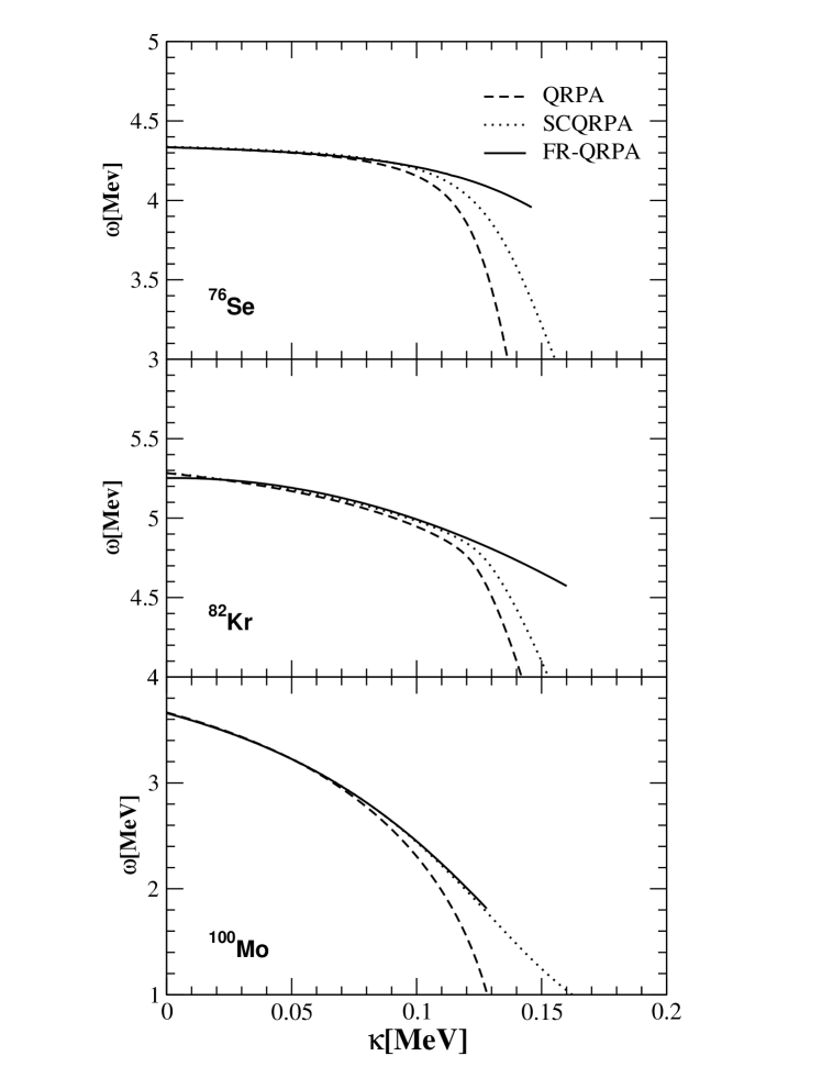
FIG. 1.: The energy of the first excited Gamow-Teller state as function of particle-particle interaction strength $\kappa$ for the daughter nuclei with $A\leq 100$

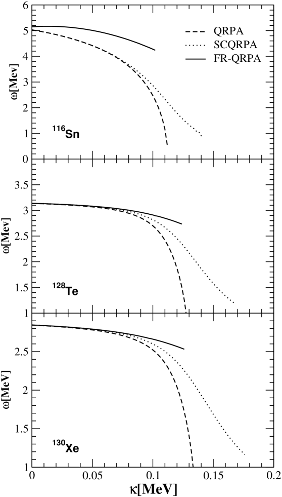
FIG. 2.: The energy of the first excited Gamow-Teller state as function of particle-particle interaction strength $\kappa$ for the daughter nuclei with $A>100$

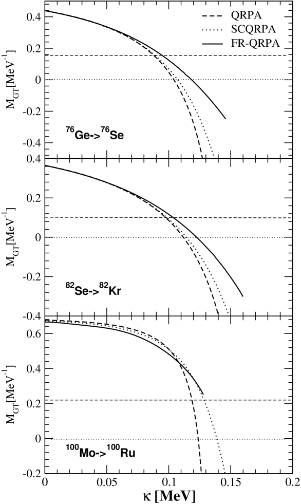
FIG. 3.: $2\nu\beta\beta$-decay matrix elements as a function of particle-particle strength $\kappa$ for $A\leq 100$ nuclei

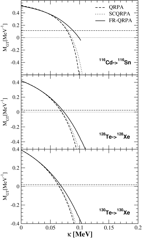
FIG. 4.: $2\nu\beta\beta$-decay matrix elements as a function of particle-particle strength $\kappa$ for nuclei with $A>100$

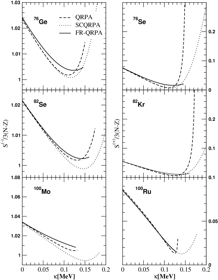
FIG. 5.: The dependence of the total $\beta^{-}$ and $\beta^{+}$ strength on the $\kappa$ parameter for mother and daughter nuclei respectively. The total strength is normalized to 3(N-Z)

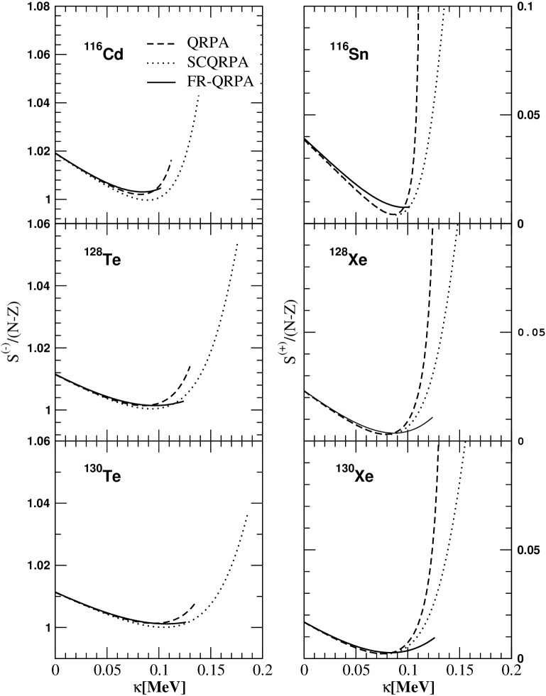
FIG. 6.: The dependence of the total $\beta^{-}$ and $\beta^{+}$ strength on the $\kappa$ parameter for mother and daughter nuclei respectively. The total strength is normalized to 3(N-Z)

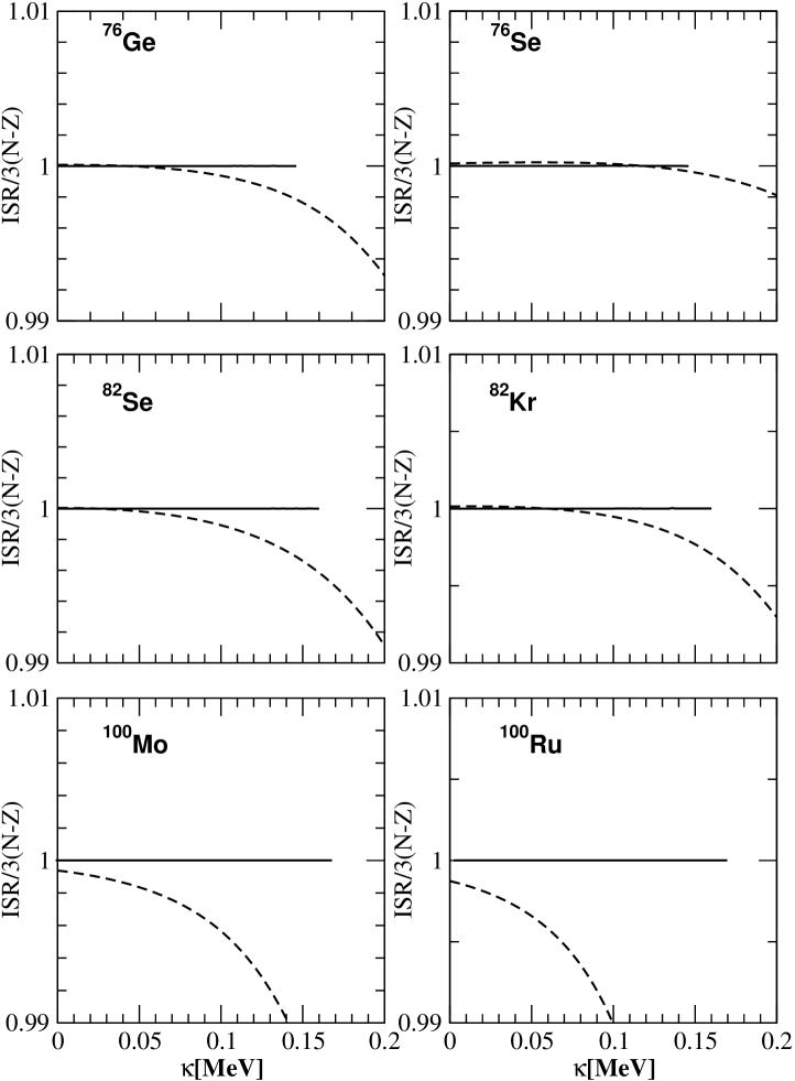
FIG. 7.: Ikeda sum rule as function of particle-particle interaction strength $\kappa$ nuclei with $A\leq 100$. The dashed line coresponds to SCQRPA and the continuous one coresponds to FRQRPA.

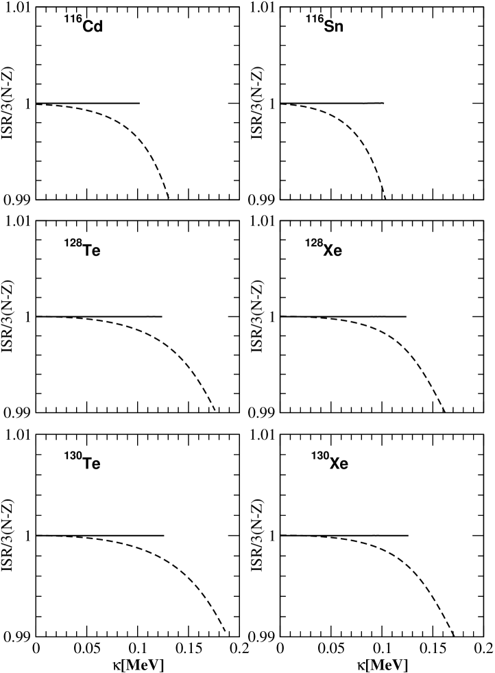
FIG. 8.: Ikeda sum rule as function of particle-particle interaction strength $\kappa$ nuclei with $A<100$. The dashed line coresponds to SCQRPA and the continuous one coresponds to FRQRPA