Solution of large scale nuclear structure problems by wave function factorization

Abstract

Low-lying shell model states may be approximated accurately by a sum over products of proton and neutron states. The optimal factors are determined by a variational principle and result from the solution of rather low-dimensional eigenvalue problems. Application of this method to $sd$-shell nuclei, $pf$-shell nuclei, and to no-core shell model problems shows that very accurate approximations to the exact solutions may be obtained. Their energies, quantum numbers and overlaps with exact eigenstates converge exponentially fast as the number of retained factors is increased.

I Introduction

Realistic nuclear structure models are difficult to solve due to the complexity of the nucleon-nucleon interaction and the sheer size of the model spaces. Exact diagonalizations are now possible for $pf$-shell nuclei Antoine ; Nathan ; Honma02 and for sufficiently light systems Navratil00 ; Navratil02 , and Quantum Monte Carlo calculations Pieper01 ; Pieper02 have solved light nuclei up to about mass $A=12$. For cases where an exact solution is not feasible, various approximations are employed. We mention stochastic methods like shell-model Monte Carlo Lang93 ; Koonin97 and Monte Carlo shell-model MCSM , and recent applications of coupled cluster expansions Heisenberg ; DeanCC .

In recent years, several truncation method for shell model diagonalizations have been developed. These methods aim at a reduction of the enormous dimensionality of shell model Hilbert spaces while maintaining a high accuracy in the computed observables. Based on arguments of statistical spectroscopy, Horoi and coworkers Horoi94 ; Horoi99 ; Horoi02 ; Horoi03 developed the exponential convergence method. Mizusaki and Imada Mizu02 ; Mizu03 devised an extrapolation method and applied it to a configuration truncation. Both techniques use single-particle basis states and provide a method to extrapolate the results of truncated calculations to the full Hilbert space. Other approaches use correlated basis states to obtain a rapid convergence. Andreozzi et al. AP ; ALP , for instance, construct a basis from products of correlated proton states and correlated neutron states. Gueorguiev et al. Vesselin01 ; Vesselin02 use a mixed-mode shell model of single-particle and collective configurations, while Vargas et al. VHD use a truncation based on coupled $SU(3)$ irreps to describe the interplay and competition of collective and single-particle degrees of freedom.

Though the selection of the relevant states is physically well motivated for all these truncation schemes, it does not directly follow from a variational principle. This is different for the density matrix renormalization group (DMRG) White92 and the very recently proposed factorization method PD03 . The DMRG uses a sophisticated renormalization and truncation scheme that includes the most important states and correlations. Dukelsky et al. Duk01 ; Duk02 and Dimitrova et al. Dimitrova02 applied this method to nuclear structure problems. The ground-state factorization is based on a related truncation. At a given truncation, the optimal states are determined from a variational principle. These last two methods also allow for an extrapolation to full Hilbert spaces as the results tend to converge exponentially. In this article we present a detailed description of the factorization method and discuss several applications. A summary of some of the main results has been presented in an earlier paper PD03 .

This article is organized as follows. In Section II we give a derivation of the main theoretical results and present details of the numerical implementation. Section III presents numerical results for $sd$-shell nuclei, $pf$-shell nuclei and for no-core shell-model problems. The convergence of the factorization method and a comparison with other truncation methods is presented in Sect. IV, and we conclude with Section V.

II Theoretical background

II.1 Motivation

Shell model basis states are products of proton Slater determinants $\{|\pi_{\alpha}\rangle,\alpha=1,\ldots,d_{P}\}$ and neutron Slater determinants $\{|\nu_{\alpha}\rangle,\alpha=1,\ldots,d_{N}\}$. Here, $d_{P}$ and $d_{N}$ denote the dimension of the proton space and the neutron space, respectively. The shell-model ground-state may be expanded as

$$|\Psi\rangle=\sum_{\alpha}^{d_{P}}\sum_{\beta}^{d_{N}}\Psi_{\alpha\beta}|\pi_{\alpha}\rangle|\nu_{\beta}\rangle.$$ (1)

This expansion is not unique since the amplitudes $\Psi_{\alpha\beta}$ depend on the choice of basis states within the two subsets. There is, however, a preferred basis in which the amplitudes $\Psi_{\alpha\beta}$ are “diagonal”. This basis is formally obtained from a singular value decomposition of the rectangular amplitude matrix $\Psi$ of dimension $d_{P}\times d_{N}$ as $\Psi=USV^{T}$. Here $U$ ($V$) is a $d_{P}\times d_{P}$ ($d_{N}\times d_{N}$) dimensional matrix with orthonormalized columns. $S$ is a rectangular matrix of dimension $d_{P}\times d_{N}$ with elements $S_{i,j}=0$ for $i\neq j$ and the “diagonal” elements $S_{i,i}=s_{i}$ are the non-negative singular values. Performing the singular value decomposition yields

$$|\Psi\rangle=\sum_{j=1}^{\min{\left(d_{P},d_{N}\right)}}s_{j}|\tilde{p}_{j}\rangle|\tilde{n}_{j}\rangle.$$ (2)

Here $s_{j}$ denote the singular values while the proton-states $|\tilde{p}_{j}\rangle$ and the neutron-states $|\tilde{n}_{j}\rangle$ are orthonormal sets of left and right singular vectors, respectively. In general, these states are superpositions of many Slater determinants and exhibit strong correlations. The non-negative singular values $s_{1}\geq s_{2}\geq s_{3}\ldots$ fulfill $\sum_{j}s_{j}^{2}=1$ due to wave function normalization.

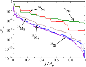
Figure 1: Singular values $s_{j}^{2}$ for ground states of ²⁰Ne ($d_{P}=66$), ²²Ne ($d_{P}=66$), ²⁴Mg ($d_{P}=495$), ²⁸Mg ($d_{P}=495$), and ²⁸Si ($d_{P}=924$).

It is interesting to compute the singular value decomposition for ground states of realistic nuclear many-body Hamiltonians. To this purpose we perform a numerical singular value decomposition of the amplitude matrix $\Psi_{\alpha\beta}$ in Eq. (1) using the Lapack routines lapack . Figure 1 shows the squares of the singular values for the ground states of $sd$-shell nuclei ²⁰Ne, ²²Ne, ²⁴Mg and ²⁸Si (from the USD interaction BW ) plotted versus their normalized index $j/d_{P}$. (We have $d_{P}=190,190,495$, and 924 for the nuclei ²⁰Ne, ²²Ne, ²⁴Mg and ²⁸Si, respectively). The singular values decrease with increasing index and rapidly become exponentially small. (Degeneracies are due to spin/isospin symmetry). This suggests that a truncation of the sum in Eq. (2) should yield an accurate approximation to the ground-state. In fact, the density matrix renormalization group (DMRG) White92 , exploits this rapid fall-off of singular values in a wave-function factorization. For obvious reasons, the expansion (2) is a factorization, and the correlated proton and neutron states are the factors. In what follows, we will devise a method that directly obtains the most important factors without knowledge of the exact ground-state.

II.2 Derivation of main results

To determine the optimal factor for a given truncation we make the ansatz

$$|\psi\rangle=\sum_{j=1}^{\Omega}|p_{j}\rangle|n_{j}\rangle$$ (3)

for the ground state. Here, the unknown factors are the proton-states $|p_{j}\rangle$ and the neutron-states $|n_{j}\rangle$. These states may be correlated and need not to be normalized. The truncation is controlled by the parameter $\Omega$ which counts the number of desired factors. Figure 1 suggests that $\Omega\ll\min{\left(d_{P},d_{N}\right)}$ yields accurate approximations to shell-model ground states. This is also the result of our numerical computations below.

Let $\hat{H}$ be the nuclear many-body Hamiltonian. To determine the unknown proton-states $|p_{j}\rangle$ and neutron-states $|n_{j}\rangle$ in Eq. (3) we consider the energy $E=\langle\psi|\hat{H}|\psi\rangle/\langle\psi|\psi\rangle$. Its variation $\delta E=0$ yields ($j=1,\ldots,\Omega$)

$$\sum_{i=1}^{\Omega}\left(\langle n_{j}|\hat{H}|n_{i}\rangle-E\langle n_{j}|n_{i}\rangle\right)|p_{i}\rangle = 0,$$

$$\sum_{i=1}^{\Omega}\left(\langle p_{j}|\hat{H}|p_{i}\rangle-E\langle p_{j}|p_{i}\rangle\right)|n_{i}\rangle = 0.$$ (4)

The solution of these nonlinear equations determines the optimal factors and the ground-state energy. Note that for fixed neutron (proton) states the first (second) set of these equations constitutes a generalized eigenvalue problem for the proton (neutron) states. To fully understand the structure of the matrices involved we rewrite the first set of the Eq. (II.2) as

$$\left(\begin{array}[]{cccc}\langle n_{1}|\hat{H}|n_{1}\rangle&\langle n_{1}|\hat{H}|n_{2}\rangle&\cdots&\langle n_{1}|\hat{H}|n_{\Omega}\rangle\\ \langle n_{2}|\hat{H}|n_{1}\rangle&\langle n_{2}|\hat{H}|n_{2}\rangle&\cdots&\langle n_{2}|\hat{H}|n_{\Omega}\rangle\\ \vdots&&\ddots&\vdots\\ \langle n_{\Omega}|\hat{H}|n_{1}\rangle&\cdots&\cdots&\langle n_{\Omega}|\hat{H}|n_{\Omega}\rangle\end{array}\right)\left(\begin{array}[]{c}|p_{1}\rangle\\ |p_{2}\rangle\\ \vdots\\ |p_{\Omega}\rangle\end{array}\right)=E\left(\begin{array}[]{cccc}\langle n_{1}|n_{1}\rangle{\hat{I}}_{P}&\langle n_{1}|n_{2}\rangle{\hat{I}}_{P}&\cdots&\langle n_{1}|n_{\Omega}\rangle{\hat{I}}_{P}\\ \langle n_{2}|n_{1}\rangle{\hat{I}}_{P}&\langle n_{2}|n_{2}\rangle{\hat{I}}_{P}&\cdots&\langle n_{2}|n_{\Omega}\rangle{\hat{I}}_{P}\\ \vdots&&\ddots&\vdots\\ \langle n_{\Omega}|n_{1}\rangle{\hat{I}}_{P}&\cdots&\cdots&\langle n_{\Omega}|n_{\Omega}\rangle{\hat{I}}_{P}\end{array}\right)\left(\begin{array}[]{c}|p_{1}\rangle\\ |p_{2}\rangle\\ \vdots\\ |p_{\Omega}\rangle\end{array}\right).$$ (21)

Here, $|p_{j}\rangle=(p_{j,1},p_{j,2},\ldots,p_{j,d_{P}})^{T}$ is a $d_{P}$-dimensional column vector (^T denotes the transpose) while ${\hat{I}}_{P}$ denotes the identity matrix in proton space. Thus,

$$\langle n_{i}|n_{j}\rangle{\hat{I}}_{P}=\left(\begin{array}[]{cccc}\langle n_{i}|n_{j}\rangle&0&\cdots&0\\ 0&\langle n_{i}|n_{j}\rangle&&0\\ \vdots&&\ddots&\vdots\\ 0&\cdots&\cdots&\langle n_{i}|n_{j}\rangle\end{array}\right)$$ (26)

is a diagonal constant matrix of dimension $d_{P}\times d_{P}$. The proton-space operators $\langle n_{i}|\hat{H}|n_{j}\rangle$ stem from the nuclear structure Hamiltonian

$$\hat{H}=\hat{H}_{N}+\hat{H}_{P}+\hat{V}_{PN},$$ (27)

with

$$\hat{H}_{N} = \sum_{n}\varepsilon_{n}\hat{a}_{n}^{\dagger}\hat{a}_{n}+{1\over 4}\sum_{n,n^{\prime},m,m^{\prime}}v_{nn^{\prime}m^{\prime}m}\hat{a}_{n}^{\dagger}\hat{a}^{\dagger}_{n^{\prime}}\hat{a}_{m}\hat{a}_{m^{\prime}},$$

$$\hat{H}_{P} = \sum_{p}\varepsilon_{p}\hat{a}_{p}^{\dagger}\hat{a}_{p}+{1\over 4}\sum_{p,p^{\prime},q,q^{\prime}}v_{pp^{\prime}q^{\prime}q}\hat{a}_{p}^{\dagger}\hat{a}^{\dagger}_{p^{\prime}}\hat{a}_{q}\hat{a}_{q^{\prime}},$$ (28)

$$\hat{V}_{PN} = \sum_{p,n,n^{\prime},p^{\prime}}v_{pnp^{\prime}n^{\prime}}\hat{a}_{p}^{\dagger}\hat{a}^{\dagger}_{n}\hat{a}_{n^{\prime}}\hat{a}_{p^{\prime}}.$$

Here, we use indices $p,q$ and $m,n$ to refer to proton and neutron orbitals, respectively. The antisymmetric two-body matrix elements are denoted as $v_{ijkl}$.

Thus, the proton-space Hamilton operator $\langle n_{i}|\hat{H}|n_{j}\rangle$ is

$$\langle n_{i}|\hat{H}|n_{j}\rangle = \sum_{p,p^{\prime}}\left(\sum_{n,n^{\prime}}v_{pnp^{\prime}n^{\prime}}\langle n_{i}|\hat{a}^{\dagger}_{n}\hat{a}_{n^{\prime}}|n_{j}\rangle\right)\hat{a}_{p}^{\dagger}\hat{a}_{p^{\prime}}$$ (29)

$$+ \langle n_{i}|\hat{H}_{N}|n_{j}\rangle+\langle n_{i}|n_{j}\rangle\hat{H}_{P}.$$

Note that the neutron-proton interaction $\hat{V}_{PN}$ results into a one-body proton operator while the neutron Hamiltonian $\hat{H}_{N}$ yields a constant. This concludes the detailed explanation of the first set of equations in Eq. (II.2). The second set has an identical structure, only the role of neutrons and protons is reversed.

II.3 Treatment of symmetries

Most modern shell-model codes use a basis of Slater determinants that preserve axial symmetry. It is straight forward to include this symmetry into the method proposed in this work. For such an “$m$-scheme” ground-state factorization we modify the ansatz (3) as

$$|\psi\rangle=\sum_{m=-M}^{M}\sum_{k=1}^{\Omega_{m}}|p_{k}(m)\rangle|n_{k}(-m)\rangle.$$ (30)

Here $|p_{k}(m)\rangle,k=1,\ldots,\Omega_{m}$ ($|n_{k}(-m)\rangle,k=1,\ldots,\Omega_{m}$) denote $d_{P,m}$ dimensional proton states ( $d_{N,-m}$ dimensional neutron states) with angular momentum projection $J_{z}=m$ ($J_{z}=-m$), and the sum over $m$ runs over all possible values of $J_{z}$. The ansatz (30) leads to a generalized eigenvalue problem similar to Eq. (II.2), with the only difference that permissible products of proton states and neutron states have zero angular momentum projection:

$$\sum_{m=-M}^{M}\sum_{k=1}^{\Omega_{m}}\bigg{(}\langle n_{k^{\prime}}(m^{\prime})|\hat{H}|n_{k}(m)\rangle$$ (31)

$$-E\langle n_{k^{\prime}}(m^{\prime})|n_{k}(m)\rangle\bigg{)}|p_{k}(-m)\rangle=0,$$

$$\sum_{m=-M}^{M}\sum_{k=1}^{\Omega_{m}}\bigg{(}\langle p_{k^{\prime}}(m^{\prime})|\hat{H}|p_{k}(m)\rangle$$ (32)

$$-E\langle p_{k^{\prime}}(m^{\prime})|p_{k}(m)\rangle\bigg{)}|n_{k}(-m)\rangle=0.$$

These equations have to be fulfilled for all possible values of $m^{\prime}$ and $k^{\prime}$. It is again useful to display the eigenvalue problem (31) for the proton states in more detail

$$\left(\begin{array}[]{ccc}\langle n(-M)|\hat{H}|n(-M)\rangle&\cdots&\langle n(-M)|\hat{H}|n(M)\rangle\\ \vdots&\ddots&\vdots\\ \langle n(M)|\hat{H}|n(-M)\rangle&\cdots&\langle n(M)|\hat{H}|n(M)\rangle\end{array}\right)\left(\begin{array}[]{c}|p(M)\rangle\\ \vdots\\ |p(-M)\rangle\end{array}\right)=E\left(\begin{array}[]{c}\langle n(-M)|n(-M)\rangle\quad|p(M)\rangle\\ \vdots\\ \langle n(M)|n(M)\rangle\quad|p(-M)\rangle\end{array}\right).$$ (42)

Here, we used the shorthands

$$|p(m)\rangle = (|p_{1}(m)\rangle,|p_{2}(m)\rangle,\cdots,|p_{\Omega_{m}}(m)\rangle)^{T},$$ (43)

the rectangular block matrices

$$\langle n(k)|\hat{H}|n(l)\rangle=$$

$$\left(\begin{array}[]{ccc}\langle n_{1}(k)|\hat{H}|n_{1}(l)\rangle&\cdots&\langle n_{1}(k)|\hat{H}|n_{\Omega_{l}}(l)\rangle\\ \vdots&\ddots&\vdots\\ \langle n_{\Omega_{k}}(k)|\hat{H}|n_{1}(l)\rangle&\cdots&\langle n_{\Omega_{k}}(k)|\hat{H}|n_{\Omega_{l}}(l)\rangle\end{array}\right),$$

and the overlap matrices

$$\langle n(k)|n(k)\rangle=$$

$$\left(\begin{array}[]{ccc}\langle n_{1}(k)|n_{1}(k)\rangle\hat{I}_{P,-k}&\cdots&\langle n_{1}(k)|n_{\Omega_{k}}(k)\rangle\hat{I}_{P,-k}\\ \vdots&\ddots&\vdots\\ \langle n_{\Omega_{k}}(k)|n_{1}(k)\rangle\hat{I}_{P,-k}&\cdots&\langle n_{\Omega_{k}}(k)|n_{\Omega_{k}}(k)\rangle\hat{I}_{P,-k}\end{array}\right).$$

Note that the right hand side of Eq. (42) is a vector. Note also that $\langle n_{i}(k)|\hat{H}|n_{j}(l)\rangle$ is a rectangular $d_{P,k}\times d_{P,l}$ matrix similar to Eq. (29), while $\hat{I}_{P,k}$ denotes the identity operator for the proton sub-space with angular momentum $J_{z}=k$. The eigenvalue problem (42) differs from the eigenvalue problem (21) due to the block diagonal overlap matrix on its right hand sight. The eigenvalue problem for the neutrons is identical to Eq. (42) when the role of neutrons and protons is reversed.

The number of factors used in the $m$-scheme factorization is given by the parameters $\Omega_{m}$. These parameters are input to the factorization. In the following, we use

$$\Omega_{m}=\Omega_{m}(\alpha)=\max{\left(1,\alpha d_{P,m}\right)},$$ (46)

and recall that $d_{P,m}$ is the dimension of the proton-subspace with angular momentum projection $J_{z}=m$. For $\alpha=0$ the most severe truncation is obtained and leads us to solve eigenvalue problems of the dimension $d_{P}$ and $d_{N}$, respectively. Setting $\alpha=1$ leads to an eigenvalue problem with the same dimension as an exact diagonalization in $m$-scheme. Below we will see that the choice (46) of parameters yields rapidly converging results. However, there may be other parameterizations that are superior. Comparison of Eq. (42) and Eq. (21) shows that the $m$-scheme factorization yields a lower-dimensional eigenvalue problem than the factorization (3) if the same number of factors is used.

Note also that a $jj$-coupled scheme can be used. Let $|p_{k}(J,m)\rangle$ ($|n_{k}(J,m)\rangle$) be a proton (neutron) state with angular momentum quantum number $J$ and angular momentum projection $J_{z}=m$. A ground-state of an even-even nucleus has $J=0$ and can be factored as

$$|\psi\rangle=\sum_{J}\sum_{m=-J}^{J}\sum_{k=1}^{\Omega_{J,m}}|p_{k}(J,m)\rangle|n_{k}(J,-m)\rangle,$$ (47)

where $\Omega_{J,m}$ is the number of retained states with angular momentum quantum number $J$ and angular momentum projection $J_{z}=m$. We choose

$$\Omega_{J,m}(\alpha)=\max{\left(1,\alpha d_{P,J,m}\right)},$$ (48)

where $d_{P,J,m}$ is the dimension of the proton-subspace with angular momentum $J$ and projection $m$. This number is independent of $m$ for fixed $J$. Generalizations of the ansatz (47) to nonzero $J$ are straight forward.

Other symmetries like parity can also be used to further reduce the dimensionality of the eigenvalue problem. Parity even states, for instance, are products of parity even proton states with parity even neutron states or products off parity odd proton states with parity odd neutron states. The ability to implement symmetries is particularly important as it widens the flexibility of the ground-state factorization. Consider for instance shell-model problems with proton and neutron spaces that differ considerably in size such that $d_{P}\ll d_{N}$. In such cases one might switch to a more symmetric factorization and factorize the ground-state as follows: one of the factor spaces would consist of neutron states that are based on a subset of neutron single-particle orbitals, while the other factor states would be based on the remaining neutron orbitals and all proton orbitals. In such a scenario, the correct implementation of the Pauli principle requires care.

II.4 Numerical solution and computational details

We discuss the solution of the eigenvalue problems. For notational convenience we focus on the solution of the equations (II.2). The corresponding equations (31) and (32) of the $m$-scheme factorization or the can be treated similarly. We solve the coupled set of nonlinear equations (II.2) in an iterative procedure. We choose a random set of linearly independent initial neutron-states $\{|n_{j}\rangle,j=1,\ldots,\Omega\}$ and construct the Hamiltonian and overlap matrix presented in Eq. (21). We then solve this generalized eigenvalue problem of dimension $\Omega d_{P}$ for those proton-states $\{|p_{j}\rangle,j=1,\ldots,\Omega\}$ that yield the lowest energy $E$. In practice, we use the sparse matrix solver Arpack arpack for this task. The solution of the generalized eigenvalue problem requires us to provide the LU factorization of the overlap matrix (i.e. the right hand side of Eq. (21)). This factorization simplifies considerably since the overlap matrix is a direct product $\hat{I}_{P}\otimes M_{N}$ and only requires the LU-factorization of the $\Omega\times\Omega$ dimensional overlap matrix $M_{N}$ with elements $\langle n_{i}|n_{j}\rangle$. We then input the resulting proton-states to the second set of Eq. (II.2). The solution of this $\Omega d_{N}$ dimensional problem yields improved neutron-states $\{|n_{j}\rangle,j=1,\ldots,\Omega\}$ and an improved (i.e. lowered) ground-state energy $E$. We iterate this procedure until the ground-state energy $E$ is converged.

For small values of $\Omega$ we typically need about 20 iterations to obtain a converged energy, and the number of iterations decreases with increasing number of kept states $\Omega$. For maximal value $\Omega=d_{N}$ , the first solution of the proton-problem (21) already yields the exact ground-state. This can be seen as follows: Using Slater determinants $\{|n_{j}\rangle=|\nu_{j}\rangle,j=1,\ldots,\Omega\}$ as input to the proton-problem (21) yields a matrix-problem that is identical in structure to the full shell-model problem.

Let us compare the effort of the ground-state factorization with an exact diagonalization. Both methods require all Hamiltonian matrix elements $\langle\pi_{\alpha}|\langle\nu_{\beta}|\hat{H}|\nu_{\gamma}\rangle|\pi_{\delta}\rangle$. The advantage of the factorization method is that the dimensionality of the eigenvalue problem is $\Omega\times\max{(d_{P},d_{N})}$ with $\Omega\ll d_{P},d_{N}$ while the dimension of the exact diagonalization scales like $d_{P}\times d_{N}$. Note that existing shell-model codes may easily be modified to include the ground-state factorization in order to obtain accurate approximations or to compute useful starting vectors for a Lanczos iteration.

It is possible to reduce the Eqs. (II.2) to a standard eigenvalue problem. For this purpose we choose a random orthonormal set of initial neutron-states $\{|n_{j}\rangle,j=1,\ldots,\Omega\}$ as input to the first eigenvalue problem. This reduces the “overlap” matrix $\langle n_{j}|n_{i}\rangle$ to a unit matrix, and we solve a standard eigenvalue problem to obtain the proton-states $\{|p_{j}\rangle,j=1,\ldots,\Omega\}$. The resulting proton-states will not be orthogonal since they are components of only one solution vector of dimension $\Omega d_{P}$. Their coefficient matrix $C$ with elements $C_{\alpha j}\equiv\langle\pi_{\alpha}|p_{j}\rangle$ may, however, be factorized in a singular value decomposition as $C=UDV^{T}$. Here $D$ denotes a diagonal $\Omega\times\Omega$ matrix while $U$ is a (column) orthogonal $d_{P}\times\Omega$ matrix, and $V$ is a orthogonal $\Omega\times\Omega$ matrix. The transformed states ($j=1,\ldots,\Omega$)

$$|p_{j}^{\prime}\rangle = \sum_{\alpha=1}^{d_{P}}U_{\alpha,j}|\pi_{\alpha}\rangle,$$

$$|n_{j}^{\prime}\rangle = \sum_{i=1}^{\Omega}V_{ij}|n_{i}\rangle$$

are orthonormal in the proton-space and in the neutron space, respectively, and they fulfill

$$|\psi\rangle=\sum_{j=1}^{\Omega}|p_{j}\rangle|n_{j}\rangle=\sum_{j=1}^{\Omega}D_{jj}|p_{j}^{\prime}\rangle|n_{j}^{\prime}\rangle.$$ (49)

The orthogonal proton-states $\{|p_{j}^{\prime}\rangle,j=1,\ldots,\Omega\}$ are then input to the second set in Eq. (II.2), which poses a standard eigenvalue problem for the neutron-states. Note that the transformed neutron states $D_{jj}|n^{\prime}_{j}\rangle$ are useful starting vectors for the Lanczos iteration of the sparse matrix solver. The resulting neutron-states should again be orthonormalized by a singular value decomposition. These singular value decompositions are very inexpensive compared to the diagonalization. Similarly, we may cast the generalized $m$-scheme eigenvalue problem (42) into a standard eigenvalue problem by enforcing orthogonality $\langle n_{k}(m)|n_{l}(m)\rangle\propto\delta_{k,l}$ between neutron states with identical angular momentum projection through the singular value decomposition.

In our implementation of the $m$-scheme factorization, we compute the matrices of the proton space operators $H_{P}$ and $\hat{a}_{p}^{\dagger}\hat{a}_{p^{\prime}}$ as well as the matrices of the neutron space operators $H_{N}$ and $\hat{a}_{n}^{\dagger}\hat{a}_{n^{\prime}}$. These sparse matrices can be stored in fast memory. The sparse matrix on the left hand side of Eq. (21) is constructed from these matrices. This sparse matrix can be kept in fast memory for sufficiently small problems; for larger problems, its nonzero matrix elements along with the row-column information can be stored in large chunks of data on disk without a severe increase of computing times.

Our implementation of the $jj$-coupled factorization is somewhat more tedious. Starting from the $m$-scheme basis states $|p_{k}(m)\rangle$ and $|n_{k}(m)\rangle$, we create basis states $|p_{k}(J,m)\rangle$ and $|n_{k}(J,m)\rangle$ with good angular momentum by numerical projection. The projection operator is Lowdin

$$\hat{P}_{J}=\prod_{j\neq J}\frac{\hat{J}^{2}-j(j+1)}{J(J+1)-j(j+1)},$$ (50)

where the product over $j$ runs over all possible angular momenta, and $\hat{J}$ denotes the angular momentum operator. The matrices of the proton Hamiltonian $H_{P}$ and the neutron Hamiltonian $H_{N}$ are then transformed to this basis and stored. The matrices of the operators $\hat{a}_{p}^{\dagger}\hat{a}_{p^{\prime}}$ and $\hat{a}_{n}^{\dagger}\hat{a}_{n^{\prime}}$ are not sparse in the basis with good $J$, and are therefore kept in the $m$-scheme basis. We perform the appropriate basis transforms in the construction of the Hamiltonian matrices.

III Numerical results

A successful application of the ground state factorization would yield accurate approximations from calculations involving rather small dimensional eigenvalue problems. Clearly, the outcome depends on the model space and the interaction under consideration. In this section we apply the $m$-scheme factorization to realistic structure calculations involving $sd$-shell nuclei, $pf$-shell nuclei and no-core shell-model computations for ⁴He. The results are compared to exact diagonalizations. We expect the method to converge most rapidly in the case of weak proton-neutron correlations. Thus, the study of $N=Z$ nuclei provides a challenging testing ground since $T=0$ proton-neutron correlations may be strong in these systems. Throughout this section $d$ denotes the dimension of the $m$-scheme eigenvalue problems (31) and (32) we actually solve, while $d_{\rm max}$ denotes the $m$-scheme dimension required for an exact solution of the problem.

III.1 $sd$-shell nuclei

We apply the $m$-scheme factorization to the $sd$-shell nuclei ²⁴Mg, ²⁶Al, ²⁸Mg, and ²⁸Al and use the USD interaction. While the factorization is particularly suited to compute accurate approximations of the ground states, we may also use it for the computation of low-lying excited states. In some cases, excited states can be obtained as a by-product of the ground-state computation. While solving the eigenvalue problems (31) and (32) for the ground-state, we may also compute excited state solutions. Let us assume that we solve the equations (31) for the proton states. The excited proton state solutions will be obtained in the presence of neutron states that are optimized for the ground state. Therefore, we expect that the excited states are less accurately reproduced than the ground-state. Figure 2 shows the resulting low-energy spectra for ²⁴Mg, ²⁸Mg, ²⁶Al, and ²⁸Al.

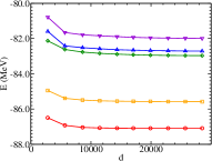
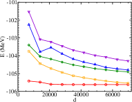
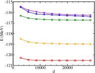
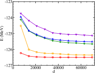
Figure 2: Low-energy spectrum of $sd$-shell nuclei versus the dimension $d$ of the eigenvalue problem. Results are obtained from targeting the ground state. Left panel: Mg isotopes ($d_{\rm max}=28503$) ²⁸Mg (top), ²⁴Mg (bottom). Right panel: Al isotopes ($d_{\rm max}=69784$) ²⁶Al (top) ²⁸Al (bottom).

The ground states converge most rapidly as more factors are retained in the factorization and the dimension $d$ of the eigenvalue problem increases. Typically, excellent results are obtained from computations involving relative dimensions $d/d_{\rm max}\approx 1/4\ldots 1/3$. For the Mg isotopes, excited states converge somewhat slower than the ground states, and level spacings are reproduced to a very good accuracy already at severe truncations. This shows that the factors of the low-lying excitations have a large overlap with the corresponding ground state factors, and we assume that this finding is related to the band structure of the low-lying excitations. The situation is different for the Al isotopes, as evident from the right panel of Fig. 2. This slower convergence of excited states is not unexpected due to the absence of band structure in these nuclei.

There are at least two approaches to improve the convergence of the excited states. In the first approach, we may target excited states by solving the eigenvalue problems (31) and (32) directly for an excited state. This method works well for the first and second excited states of ²⁴Mg, as shown in Fig. 3. However, this approach is unstable for higher excited states of ²⁴Mg and for the first excited state of ²⁶Al, as the solutions of the eigenvalue problem are oscillating but fail to converge with increasing number of iterations. In the case of ²⁶Al we proceed as follows. The ground state has angular momentum $J=5$ while the first excited state has angular momentum $J=0$. We may thus use the $jj$-coupled ansatz (47) to compute the lowest-lying state with angular momentum $J=0$. This yields the first excited state. Figure 4 shows the results plotted versus the corresponding $m$-scheme dimension. The convergence is much improved and comparable to that of the ground-state.

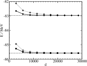
Figure 3: . Energies of the first and second excited states of ²⁴Mg versus the dimension of the eigenvalue problem. Hollow data points: results from targeting the ground state. Filled data points: results from directly targeting the excited states. Dashed lines: exact results.

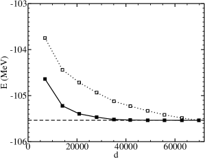
Figure 4: Energy of the first excited state of ²⁶Al versus the dimension of the eigenvalue problem. Hollow data points: results from targeting the ground state. Filled data points: ground state calculation for zero angular momentum. Dashed line: exact result.

So far we have only focused on the energies. In the remainder of this section we discuss how the states and their quantum numbers are reproduced by the factorization. For ²⁴Mg we analyze the wave-function structure of the low-lying levels. Figure 5 shows the squared overlaps with the exact results, obtained from targeting the ground state. The solution of an eigenvalue problem of only 10% of the full dimension $d_{\rm max}$ already yields between 90-96% of squared overlap. The directly targeted ground-state is reproduced to more than 99% once the dimension exceeds 20% of the full dimension $d_{\rm max}$. The inset of Fig. 5 shows that the defect $1-\langle\psi_{\rm exact}|\psi_{\rm factor}\rangle^{2}$ decreases exponentially fast as more factors are retained. While the convergence is best for the directly targeted ground-state, the excited states are also very accurately reproduced.

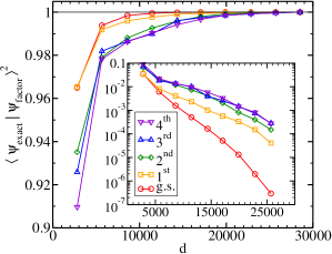
Figure 5: Squared overlaps $\langle\psi_{\rm exact}|\psi_{\rm factor}\rangle^{2}$ for the low-lying states in ²⁴Mg versus the dimension of the eigenvalue problem (from targeting the ground state). The inset shows the deviation $1-\langle\psi_{\rm exact}|\psi_{\rm factor}\rangle^{2}$ versus the dimension of the eigenvalue problem.

Let us also verify for ²⁴Mg that the quantum numbers of the low-lying states are reproduced correctly. Due to rotational symmetry, the expectation value for the angular momentum should fulfill

$$\langle\hat{J}^{2}\rangle=j(j+1),$$ (51)

where $j$ is a nonnegative integer. Figure 6 shows the $j$-values of the low-lying states for ²⁴Mg. The results were obtained by targeting the ground state. The angular-momenta are very accurately reproduced once about 20% of the states are retained in the factorization. This is remarkable since rotational symmetry is not enforced in the $m$-scheme factorization, and no kind of constraint or projection was used. Similar results are obtained for the total isospin and for other $sd$-shell nuclei. The accurate reproduction of quantum numbers, wave-functions and energies implies that transition matrix elements can accurately be computed. This concludes or detailed discussion of ²⁴Mg.

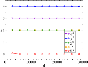
Figure 6: Angular momentum value $j$ for the low-lying states in ²⁴Mg versus the dimension of the eigenvalue problem (from targeting the ground state).

We finally mention that we also compared the $m$-scheme factorization with the $jj$-coupled scheme. For ²⁴Mg we find practically identical convergence of the ground-state energy when plotted versus the relative dimension $d/d_{\rm max}$ of the corresponding eigenvalue problem. The dimensions $d$, $d_{\rm max}$ of the eigenvalue problem in the $jj$-coupled scheme are, of course, smaller than for the $m$-scheme. However, this does not translate directly into a computational speed-up since the $jj$-scheme algorithm is more complex and involves less sparse matrices. We believe that its main advantage consists of the possibility to directly target the lowest state with a given angular momentum.

III.2 $pf$-shell nuclei

Many theoretical results for $pf$-shell nuclei are available from exact calculations for the KB3 interaction. In the lower $pf$-shell, diagonalizations can be based on an $m$-scheme basis Antoine . The $m$-scheme dimensions of upper $pf$-shell nuclei exceed one billion, and exact diagonalizations have been performed in a $J=0$ coupled basis Nathan , reducing the dimensions to the order of ten million. In this section we compare the results from $m$-scheme factorization with the exact results. We are particularly interested in the efficiency of the method and would like to answer the following question. How does the relative dimension $d/d_{\rm max}$, at which an accurate approximation to the ground state is obtained, scale with increasing dimension $d_{\rm max}$ required for an exact diagonalization?

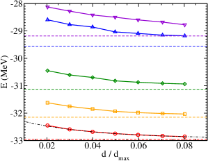
Figure 7: Data points: Low-lying energies of ⁴⁸Cr (KB3 interaction) versus the dimension $d$ of the eigenvalue problem relative to the $m$-scheme dimension $d_{\rm max}$. Dashed lines: Exact results. Dashed-dotted line: Exponential fit $E(d/d_{\rm max})=-32.92+0.851\exp{(-31.38\,d/d_{\rm max})}$ to the ground state energy.

For $pf$-shell nuclei we use the KB3 interaction KB . Figure 7 shows the low-lying energies for ⁴⁸Cr plotted versus the relative dimension $d/d_{\rm max}$ of the eigenvalue problem. The exact ground state energy is $E_{0}=-32.95$ MeV and results from the solution of an eigenvalue problem with dimension $d_{\rm max}=1.96\times 10^{6}$ Antoine . The ground-state energy converges exponentially quickly as the number of retained factors increases. The right-most data point results from an eigenvalue problem with only 8% of the $m$-scheme dimension and involves $\Omega=\sum_{m}\Omega_{m}=391$ factors. It deviates less than 100 keV from the result of an exact diagonalization. An exponential fit of the form $E(d/d_{\rm max})=a+b\exp{(-cd/d_{\rm max})}$ to the right-most six data points yields the estimate $E(1)=-32.92$ MeV, which is only 30 keV above the exact result. The excited states are obtained from targeting the ground state. The level spacings of the two lowest excitations are very accurately reproduced even at the most severe truncation, while the spacings to the higher levels are about 200-300 keV too large. The angular momentum expectation values are plotted in Fig. 8. For $d/d_{\rm max}\gtrsim 0.04$, energies and quantum numbers are sufficiently well converged. Considering the modest size of the eigenvalue problem we solved, these are very good results.

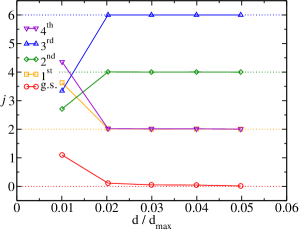
Figure 8: Angular momentum value $j$ for the low-lying excitations of the $pf$-shell nucleus ⁴⁸Cr (KB3 interaction) plotted versus the dimension $d$ of the eigenvalue problem relative to the $m$-scheme dimension $d_{\rm max}$. The dotted lines are the exact results.

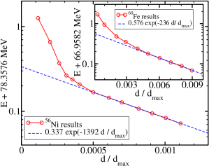
Figure 9: Ground-state energy $E$ versus the dimension $d$ of the eigenvalue problem relative to the $m$-scheme dimension $d_{\rm max}\approx 1.09\times 10^{9}$ for ⁵⁶Ni. The data points are from the $m$-scheme factorization, and the dashed line is an exponential fit to the data. Inset: Similar plot for ⁶⁰Fe ($d_{\rm max}\approx 110\times 10^{6}$).

After this detailed discussion of ⁴⁸Cr, we factor the ground states of ⁶⁰Fe and ⁵⁶Ni. The exact energies are $E=-67.0$MeV and $E=-78.46$MeV, respectively Nathan , and the corresponding $m$-scheme dimensions are $d_{\rm max}\approx 110\times 10^{6}$ and $d_{\rm max}\approx 1.09\times 10^{9}$, respectively. Fig. 9 shows that the ground states of these nuclei can very efficiently be factored. Using an exponential fit to the numerical data points, the ground state energies are reproduced within a deviation of 50 keV for ⁶⁰Fe and 100 keV for ⁵⁶Ni. Most importantly, the relative dimension of the eigenvalue problem we solve is $d/d_{\rm max}\approx 1\%$ for ⁶⁰Fe (from $\Omega=\sum_{m}\Omega_{m}=352$ states) and about $d/d_{\rm max}\approx 0.1\%$ for ⁵⁶Ni (from $\Omega=\sum_{m}\Omega_{m}=147$ states). This suggests that the factorization gets increasingly efficient as the dimension of the problem increases.

III.3 No-core shell model

As a final test, we consider a no-core shell-model problem and apply the $m$-scheme factorization to ⁴He using a manageable model space and a realistic interaction from a $G$-matrix calculation. The model space consists of the 0$s$-0$p$-1$s$-0$d$-0$f$-1$p$ shells. The $G$-matrix stems from a 15$\hbar\omega$ calculation and is based on the Idaho-A potential IdahoA . The Idaho-A potential is derived from an effective Lagrangian that respects QCD inspired chiral symmetry. We calculate the $G$-matrix from

$$G(\omega)=V+\frac{1}{\omega-QTQ}G(\omega)$$ (52)

where $\omega$ is the starting energy, $T$ is the kinetic energy operator, and $Q$ is the Pauli operator. Our Pauli operator allows for all allowed configurations to be active in the chosen model space. We also employ folded-diagrams calculated at $\tilde{\omega}=-20.0$ MeV to decrease the dependence of the resulting two-body interaction on the starting energy. Details concerning the derivation of the $G$-matrix may be found in Ref. hj95 . We also include center-of-mass corrections perturbatively. Finally, we employ the method of Ref. dean99 to obtain an interaction that yields a ground-state energy that is approximately free of center-of-mass contamination. Note that this small space is not sufficient to completely describe the ⁴He nucleus, but still illustrates the power of the factorization method for problems in which the core is absent.

Figure 10 shows the energies for the three lowest lying states of ⁴He versus the dimension $d$ of the eigenvalue problem we solve. The results for the excited states were obtained while targeting the ground state. The exact results are obtained from a diagonalization with $m$-scheme dimension $d_{\rm max}=79298$. Note that the ground state and the excited states converge very fast toward the exact results. A calculation with $d/d_{\rm max}\approx 0.2$ already yields excellent approximations, and the angular momentum quantum numbers are converged.

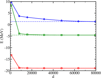
Figure 10: Energies of low-lying states of ⁴He plotted versus the dimension $d$ of the eigenvalue problem. The dashed lines are the exact results.

Let us finally suggest an alternative treatment of the center of mass problem. The center of mass is separable in an oscillator basis where all many-body states with up to $N_{\rm max}$ oscillator quanta are included. The factorization could be applied in this scheme by combining proton states with $n$ oscillator quanta and neutron states with $n^{\prime}$ oscillator quanta such that $n+n^{\prime}\leq N_{\rm max}$.

IV Convergence of the method

IV.1 Convergence properties

The results of the preceding section showed that the factorization converges exponentially quickly as more factors are retained. So far we considered nuclei with equal dimension of proton space and neutron space, most of them being $N=Z$ nuclei. What can be expected for other cases? To answer this important question, we computed the exact ground states of several $pf$-shell nuclei and numerically performed singular value decompositions of their amplitude matrices $\Psi_{\alpha\beta}$ as defined in Eq. (1). Fig. 11 shows logarithmic plots of the resulting singular value spectra. The singular value spectra exhibit a very sharp initial falloff followed by an exponential decay. The initial falloff is stronger for larger dimension of the proton space $d_{P}$, and this renders the factorization method very effective. There is no clear trend for isotopic chains. The singular value spectra of the lighter $pf$-shell nuclei decay most rapidly for the $N=Z$ nuclei, while the decay is faster for mid-shell nuclei away from $N=Z$. Our results suggest that the application of the factorization method is not limited to $N=Z$ nuclei. We also computed the number of factors, $\Omega(x)$, such that $\sum_{j=1}^{\Omega(x)}s_{j}^{2}>x$ for $x=0.99$ and $x=0.999$. The results of Table 1 show that the factorization of all these nuclei should converge rapidly as more factors are included. Larger dimensional model spaces usually require the retention of more factors, but the ratio $\Omega(x)/\min{(d_{P},d_{N})}$ decreases with increasing size of the problem. Note that ⁴⁸Cr is relatively difficult to factor into proton and neutron states. This suggests that this nucleus exhibits particularly strong proton-neutron correlations.

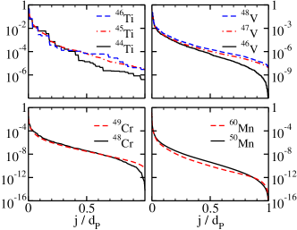
Figure 11: Singular value spectra (squared singular values $s_{j}^{2}$) for ground states of Ti isotopes (upper left, $d_{P}=190$), V isotopes (upper right, $d_{P}=1140$), Cr isotopes (lower left, $d_{P}=4845$), and ⁵⁰Mn (lower right, $d_{P}=15504$).

Nucleus	$d_{P}$	$d_{N}$	$\Omega(0.99)$	$\Omega(0.999)$
44Ti	190	190	40	75
45Ti	190	1140	45	109
46Ti	190	4845	43	126
46V	1140	1140	98	270
47V	1140	4845	111	324
48V	1140	15504	151	392
48Cr	4845	4845	258	775
49Cr	4845	15504	168	619
50Mn	15504	15504	197	821
60Mn	15504	15504	163	570

Table 1:

Proton space dimension $d_{P}$ and neutron space dimension $d_{N}$ for various $pf$-shell nuclei. $\Omega(x)$ denotes the number of factors that have to be retained for an overlap $\sum_{j=1}^{\Omega}s_{j}^{2}=x$ with the exact ground state.

We recall that the $m$-scheme factorization (30) requires as input the number of factors with a given angular momentum projection, $\Omega_{m}$, which were taken according to Eq. (46). It is interesting and important to check this choice of input parameters. To this purpose we compare the singular value spectrum from the factorization with the singular value spectrum from an exact calculation. The factorization was performed for ⁴⁸Cr using $\alpha=0.04$ and $\alpha=0.08$ in Eq. (46). These truncations included a total of $\Omega=\sum_{m}\Omega(\alpha)=197$ and $\Omega=391$ factors, respectively. Figure 12 compares the resulting singular value spectra with the singular value decomposition of the exact ground state. The agreement between the exact results and the approximations is rather good, and improves with increasing number of retained factors. Note however, that the smaller singular values deviate from each other. This suggests, that it should be possible to somewhat improve the choice of input parameters $\Omega_{m}$.

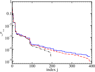
Figure 12: Singular value spectra (squared singular values $s_{j}^{2}$) for ⁴⁸Cr. Singular value decomposition of exact ground state (full line), $m$-scheme factorization using $\Omega=391$ factors (dashed line), and $\Omega=197$ factors (dashed-dotted line).

We finally mention that we lack an understanding about the rapid initial falloff in singular value spectra. For the Hamiltonians considered in this work the falloff is evident. Moreover, the results obtained from DMRG calculations over the past decade demonstrate that density-matrix spectra decay rapidly for the ground states of a large number of relevant Hamiltonians. A few works address the theoretical foundations of the DMRG. Peschel and coworkers investigated density matrix spectra of several soluble problems Peschel , while Okunishi et al. discussed the asymptotic behavior of density matrix eigenvalues for noncritical spin systems Okunishi . Östlund and Rommer showed that if the DMRG renormalization converges to a fixed point, the DMRG ground-state is of a special matrix-product form Ostlund . Given the lack of generally valid analytical results, it is thus interesting to numerically investigate singular value spectra for “generic” Hamiltonians. For this purpose we considered the model space of $pf$-shell nuclei ⁴⁴Ti and ⁴⁶V and used a random two-body interaction that preserves spin and isospin, i.e. the spin/isospin coupled two-body matrix elements $V_{\alpha,\beta}$ are independent Gaussian random variables with zero mean $\langle V_{\alpha,\beta}\rangle=0$ and variance $\langle V_{\alpha,\beta}V_{\alpha^{\prime},\beta^{\prime}}\rangle=(\delta_{\alpha,\alpha^{\prime}}\delta_{\beta,\beta^{\prime}}+\delta_{\alpha,\beta^{\prime}}\delta_{\beta,\alpha^{\prime}})$. For a realistic choice of the single-particle energies we find singular value spectra that are similar to the realistic spectra. However, setting all single-particle energies to zero yields singular value spectra with longer tails and a less rapid decay.

IV.2 Comparison with other truncation methods

In recent years, several truncation methods have been developed for and applied to shell model problems. In this subsection we compare some of these approaches with the method presented in this work. This comparison focuses on convergence and accuracy of low-lying energy spectra at a given level of truncation.

We start with the DMRG which also bases its truncation on the singular values White92 . Dukelsky and coworkers applied the DMRG to nuclear structure problems involving pairing Duk01 and pairing-plus-quadrupole interactions Duk02 . These applications were very successful as accurate results could be obtained for huge Hilbert spaces. The factorization method proposed in this work can only treat much smaller Hilbert spaces and cannot compete with the DMRG for these systems. However, the recent DMRG calculation Dimitrova02 for the realistic nuclear structure problem (²⁴Mg with USD interaction) converges very slowly.

Recently, Andreozzi et al. AP ; ALP used a small number of correlated proton states and correlated neutron states as a truncated basis for shell model problems. The correlated proton (neutron) states are the low-energy eigenstates of the proton-proton (neutron-neutron) Hamiltonian. The full shell model Hamiltonian including the proton-neutron interaction is then solved in this space. Andreozzi and Porrino report exponentially converging results and a considerable reduction in the number of basis states AP . This procedure differs from our approach mainly by the absence of a variational principle.

A third related method is the exponential convergence method (ECM) developed by Horoi and coworkers Horoi94 ; Horoi99 ; Horoi02 ; Horoi03 . In this method, shell-model configurations are ordered according to their average centroid, which are obtained from statistical spectroscopy. This ordering gives a natural truncation scheme, and analytical arguments suggest an exponential convergence of energies with increasing number of retained configurations. Once the exponential region is identified, the full space energies can be extrapolated by an exponential fit. A direct comparison is not easy since the FPD6 interaction is used for $pf$-shell nuclei, and since ECM results are plotted versus $JT$-coupled dimension of the truncated space. We believe, however, that our method converges more rapidly than the ECM. For ⁴⁸Cr, for instance, our rate of exponential convergence is $c\approx-31.38$ (See Fig. 7), which is about a factor eight larger than what is reported for the ECM in Fig. 1 of Ref. Horoi02 . For ⁵⁶Ni, our exponential rate is about a factor 200 larger than the ECM rate HoroiPC , and our identification of the exponential region requires a $m$-scheme dimension $d\approx 10^{6}$ (See Fig. 10) while the ECM requires an $m$-scheme dimension of 4-5 million HoroiPC .

For upper $pf$-shell nuclei, truncations can be based on the maximal number $t$ of nucleons outside the $f_{7/2}$ subshell Caurier . Within this truncation, the convergence of the energy is rather slow, and it is difficult to extrapolate from results in truncated spaces to the full Hilbert space. Mizusaki and Imada devised extrapolation methods that link the error due to the truncation to the variance of the energy in the truncated space. This approach lead to a first order Mizu02 and a second-order extrapolation method Mizu03 for predictions of low-lying states in various $pf$-shell nuclei. For ⁵⁶Ni the approximation of a closed $f_{7/2}$ subshell is well justified, and the extrapolation methods yields results that are superior to the factorization MizusakiPC . For ⁴⁸Cr, however, the factorization seems to be of advantage: The exact ground-state energy being $E=-32.95$ MeV and the $m$-scheme dimension $d=1.96\times 10^{6}$. The first-order extrapolation method Mizu02 yields $E=-33.008$ for $t=5$ and $E=-32.975$ for $t=6$, and the corresponding $m$-scheme dimensions are $d(t=5)\approx 1.3\times 10^{6}$ and $d(t=6)\approx 1.76\times 10^{6}$. The second-order extrapolation (“scheme I”) Mizu03 yields $E=-32.91$ for $t=5$. Slightly better results are obtained from a different truncation scheme (“scheme II”). The ground-state factorization yields a comparably good energy estimate $E=-32.92$ MeV (See Fig. 7) from solving a much smaller eigenvalue problem of dimension $d=1.6\times 10^{5}$.

The mixed-mode shell model approach developed by Gueorguiev et al Vesselin01 ; Vesselin02 combines single-particle configuration and $SU(3)$ collective configurations to describe the interplay and competition between single-particle and collective degrees of freedom. For the $sd$-shell nucleus ²⁴Mg, the mixed-mode shell model yields good approximations to the binding energy (within 2% deviation of the exact result), and low-energy configurations which exceed 90% overlap with the exact results. These results stem from a truncated space of only 10% the full Hilbert space Vesselin02 . At the 10% level of the truncation, the factorization method yields an energy deviation of less than 1% (See Fig. 2), and squared overlaps exceed 96% for the two lowest lying states and 90% for the following three states (See Fig. 5).

The method proposed in this work thus compares well to most of the alternatives regarding convergence and accuracy at a given level of truncation. Note, however, that its implementation seems somewhat more complex than a shell-model approach with a configuration truncation and somewhat less complex than the DMRG algorithm.

V Conclusion

We approximated the ground states of realistic nuclear structure Hamiltonians by sums over products of correlated proton states and correlated neutron states. The optimal states are determined by a variational principle and are the solution of rather low-dimensional eigenvalue problems. Computations for $sd$-shell nuclei, $pf$-shell nuclei, and no-core shell models show that the method converges exponentially quickly as more factors are included, and that accurate approximations to shell-model ground states and low-lying excitations may be obtained. For the largest problems we considered, the dimension of the eigenvalue problem was reduced by three orders of magnitude. Momentarily, the application of this method is limited by the size of the proton space and the neutron space. An interesting future development would also consider the factorization of these spaces in order to treat larger dimensional problems. While the reason of the exponential convergence is not yet understood, computations of shell model problems with realistic and random two-body interactions suggest that this behavior can be expected for a variety of interactions.

References

- (1) E. Caurier, A. P. Zuker, A. Poves, and G. Martínez-Pinedo, Phys. Rev. C50, 225 (1994), nucl-th/9307001.
- (2) E. Caurier, G. Martínez-Pinedo, F. Nowacki, A. Poves, J. Retamosa, and A. P. Zuker, Phys. Rev. C59, 2033 (1999), nucl-th/9809068.
- (3) M. Honma, T. Otsuka, B. A. Brown, and T. Mizusaki, Phys. Rev. C65, 061301(R) (2002), nucl-th/0205033.
- (4) P. Navrátil, J. P. Vary, and B. R. Barrett, Phys. Rev. Lett. 84 (2000) 5728, nucl-th/0004058; Phys. Rev. C62, 054311 (2000).
- (5) P. Navrátil and W. E. Ormand, Phys. Rev. Lett. 88, 152502 (2002).
- (6) S. C. Pieper and R. B. Wiringa, Ann. Rev. Nucl. Part. Sci. 51, 53 (2001), nucl-th/0103005.
- (7) S. C. Pieper, K. Varga, R. B. Wiringa, Phys. Rev. C66,044310 (2002), nucl-th/0206061.
- (8) G. H. Lang, C. W. Johnson, S. E. Koonin, and W. E. Ormand, Phys. Rev. C48, 1518 (1993), nucl-th/9305009.
- (9) S. E. Koonin, D. J. Dean, and K. Langanke, Phys. Rep. 278, 1 (1997), nucl-th/9602006.
- (10) M. Honma, T. Mizusaki, and T. Otsuka, Phys. Rev. Lett. 75, 1284 (1995), nucl-th/9609043.
- (11) J. H. Heisenberg and B. Mihaila, Phys. Rev. C59, 1440 (1999), nucl-th/9802029.
- (12) D.J. Dean and M. Hjorth-Jensen, AIP Conference Proceedings 656, 197 (2003), nucl-th/0208053.
- (13) M. Horoi, B. A. Brown, and V. Zelevinsky, Phys. Rev. C50, R2274 (1994), nucl-th/9406004.
- (14) M. Horoi, A. Voyla, and V. Zelevinsky, Phys. Rev. Lett. 82, 2064 (1999), nucl-th/9806015.
- (15) M. Horoi, B. A. Brown, and V. Zelevinsky, Phys. Rev. C65, 027303 (2002).
- (16) M. Horoi, B. A. Brown, and V. Zelevinsky, Phys. Rev. C67, 034303 (2003).
- (17) T. Mizusaki and M. Imada, Phys. Rev. C65, 064319 (2002), nucl-th/0203012.
- (18) T. Mizusaki and M. Imada, Phys. Rev. C67, 041301(R) (2003), nucl-th/0302059.
- (19) F. Andreozzi and A. Porrino, J. Phys. G 27, 845 (2001), nucl-th/9906070.
- (20) F. Andreozzi, N. Lo Iudice, and A. Porrino, nucl-th/0307046
- (21) V. G. Gueorguiev, J. P. Draayer, and C. W. Johnson, Phys. Rev. C63, 014318 (2001), nucl-th/0009014.
- (22) V. G. Gueorguiev, W. E. Ormand, C. W. Johnson, and J. P. Draayer, Phys. Rev. C65, 024314 (2002), nucl-th/0110047.
- (23) C. E. Vargas, J. G. Hirsch, and J. P. Draayer, Nucl. Phys. A 690, 409 (2001), nucl-th/0009050.
- (24) S. R. White, Phys. Rev. Lett. 69, 2863 (1992); Phys. Rev. B48, 10345 (1993).
- (25) T. Papenbrock and D. J. Dean, Phys. Rev. C67, 051303(R) (2003), nucl-th/0301006.
- (26) J. Dukelsky and S. Pittel, Phys. Rev. C63, 061303 (2001), nucl-th/0101048.
- (27) J. Dukelsky and S. Pittel, S. S. Dimitrova, and M. V. Stoitsov, Phys. Rev. C65, 054319 (2002), nucl-th/0202048.
- (28) S. S. Dimitrova, S. Pittel, J. Dukelsky, and M. V. Stoitsov, nucl-th/0207025.
- (29) E. Anderson, Z. Bai, C. Bischof, S. Blackford, J. Demmel, J. Dongarra, J. Du Croz, A. Greenbaum, S. Hammarling, A. McKenney, and D. Sorensen, LAPACK User’s Guide, Edition (SIAM, Philadelphia 1999).
- (30) B. A. Brown and B. H. Wildenthal, Ann. Rev. Nucl. Part. Sci. 38, 29 (1988).
- (31) P. O. Löwdin, Rev. Mod. Phys. 36, 966 (1964).
- (32) T. T. S. Kuo and G. E. Brown, Nucl. Phys. A 114, 241 (1968); A. Poves and A. P. Zuker, Phys. Rep. 70, 235 (1980).
- (33) R. B. Lehoucq, D. C. Sorensen, and C. Yang, ARPACK User’s Guide (SIAM, Philadelphia 1998).
- (34) D.R. Entem and R. Machleidt, Phys. Lett. B524, 93 (2002).
- (35) M. Hjorth-Jensen, T.T.S. Kuo, and E. Osnes, Phys. Reps, 261, 125 (1995).
- (36) D.J. Dean, M.T. Ressell, M. Hjorth-Jensen, S.E. Koonin, K. Langanke, and A.P. Zuker, Phys. Rev. C 59, 2474 (1999).
- (37) I. Peschel and M.-C. Chung, J. Phys. A 32, 8419 1999, cond-mat/9906224; I. Peschel, M. Kaulke and Ö. Legeza, Ann. Phys. (Leipzig) 8, 153 (1999), cond-mat/9810174; M.-C. Chung and I. Peschel, Phys. Rev. B62, 4191 (2000), cond-mat/0004222; Phys. Rev. B64, 064412 (2001), cond-mat/0103301.
- (38) K. Okunishi, Y. Hieida, and Y. Akutsu, Phys. Rev. E59, R6227 (1999), cond-mat/9810239.
- (39) S. Östlund and S. Rommer, Phys. Rev. Lett. 75, 3537 (1995); S. Rommer and S. Östlund, Phys. Rev. B55, 2164 (1997), cond-mat/9606213.
- (40) M. Horoi, private communication.
- (41) E. Caurier, F. Nowacki, A. P. Zuker, G. Martínez-Pinedo, A. Poves, and J. Retamosa, Nucl. Phys. A 654, 747c (1999).
- (42) T. Mizusaki, private communication.