KEWPIE: a dynamical cascade code for decaying exited compound nuclei

Abstract

A new dynamical cascade code for decaying hot nuclei is proposed and specially adapted to the synthesis of super-heavy nuclei. For such a case, the interesting channel is the tiny fraction that will decay through particles emission, thus the code avoids classical Monte-Carlo methods and proposes a new numerical scheme. The time dependence is explicitely taken into account in order to cope with the fact that fission decay rate might not be constant. The code allows to evaluate both statistical and dynamical observables. Results are successfully compared to experimental data.

PACS numbers: 24.60.Dr,25.70.Jj,25.85.-w

I Introduction

Since the pioneering work of Bateman [1] who developed a general equation for radioactive decay chains, the model has found many applications in nuclear physics and in other fields. Purely statistical version of the problem, when the time is integrated out, has been extended to multi-channel cascade process of decay of exited compound nuclei that can evaporate neutrons, protons, alphas… and successfully compared to experimental data. The original time dependent Bateman equations can also easily be extended to the multi-channel process, provided that the decay widths are time-independent. However, the decay width of the fission channel is now known not to be time-independent, so Bateman problem should be solved numerically. Actually in fission of excited compound nuclei, it is known that it takes a finite time to build up the quasi-stationary probability flow over the fission barrier. Therefore, the time evolution should be taken into account. For recent reviews on the dynamics of fission, see Refs. [2, 3].

One of our purposes is to apply the method to evaluate the production cross section of the superheavy elements. In such reactions, most of the compound nuclei will undergo fission, and thus we need to evaluate the very tiny fraction that will decay only through particles emission. Therefore, classical Monte-Carlo methods [4, 5] are not suitable. We propose here another numerical scheme. Furthermore we construct a new statistical code named KEWPIE (Kyoto Evaporation Width calculation Program with tIme Evolution).

Fusion reactions that lead to the production of super-heavy elements involve often a combination of rather heavy ions for the entrance channel where it is well known that fusion is strongly hindered. The extra push parametrisation gives only a qualitative behaviour of this fusion hindrance, so more precise calculation should be done. There are several way of taking into account the hindrance, one of which is to use the two step model [6, 7, 8]. The code is designed to accommodate fusion probabilities calculated by such a model, in addition to the probabilities given as usual by transmission coefficients whose calculation with the full proximity potential is included in the code as standard.

II Dynamical framework

A Single chain

1 Populations as a function of time

Before generalising the method to the multi-channel decay problem, we first recall Bateman’s results considering a single chain starting from a single nucleus. The equations then read,

$$\frac{dP_{1}}{dt} = -\Gamma^{t}_{1}P_{1}\quad{\rm with}\quad P_{1}(0)=1,$$ (1)

$$\frac{dP_{2}}{dt} = \Gamma_{1}P_{1}-\Gamma^{t}_{2}P_{2}\quad{\rm with}\quad P_{2}(0)=0$$ (2)

$$\frac{dP_{3}}{dt} = \Gamma_{2}P_{2}-\Gamma^{t}_{3}P_{3}\quad{\rm with}\quad P_{3}(0)=0$$ (3)

$$\vdots$$ (4)

$$\frac{dP_{n}}{dt} = \Gamma_{n-1}P_{n-1}-\Gamma^{t}_{n}P_{n}\quad{\rm with}\quad P_{n}(0)=0,$$ (5)

where $\Gamma^{t}_{n}$ is the total decay width for the nucleus $n$ and $\Gamma_{n}$ is the evaporation width, whatever the particle is. $P_{n}(t)$ denotes the population of the nucleus $n$ at time $t$. If the decaying widths are time independent, it is very easy to solve analytically these coupled differential equations, by taking the Laplace transform as Bateman did. This leads to

$$\tilde{P}_{1}(s) = \frac{1}{\Gamma^{t}_{1}+s}$$ (6)

$$\tilde{P}_{2}(s) = \frac{1}{\Gamma^{t}_{2}+s}\frac{\Gamma_{1}}{\Gamma^{t}_{1}+s}$$ (7)

$$\vdots$$ (8)

$$\tilde{P}_{n}(s) = \frac{1}{\Gamma^{t}_{n}+s}\prod_{i=1}^{n-1}\frac{\Gamma_{i}}{\Gamma^{t}_{i}+s},$$ (9)

where $\tilde{P}(s)$ is the Laplace transform of $P(t)$. The solution is then obtained by taking the inverse Laplace transform,

$$P_{1}(t) = e^{-\Gamma^{t}_{1}t}$$ (10)

$$P_{2}(t) = \frac{\Gamma_{1}}{\Gamma^{t}_{2}-\Gamma^{t}_{1}}(e^{-\Gamma^{t}_{1}t}-e^{-\Gamma^{t}_{2}t})$$ (11)

$$\vdots$$ (12)

$$P_{n}(t) = \prod_{k=1}^{n-1}\Gamma_{k}\sum_{i=1}^{n}\frac{e^{-\Gamma^{t}_{i}t}}{\prod_{j\neq i}(\Gamma^{t}_{j}-\Gamma^{t}_{i})},$$ (13)

where we have supposed that the $\Gamma^{t}_{n}$’s are all different from each other. A special attention should be drawn on the last nucleus of the chain, for which the solution might differ from the above when $\Gamma^{t}_{n_{max}}=0$. For such a case,

$$P_{n_{max}} = \Gamma_{n_{max}-1}\int_{0}^{+\infty}dt\,P_{n_{max}-1}(t)$$ (14)

$$= \prod_{k=1}^{n_{max}-1}\Gamma_{k}\sum_{i=1}^{n_{max}}\frac{1-e^{-\Gamma^{t}_{i}t}}{\Gamma^{t}_{i}\prod_{j\neq i}(\Gamma^{t}_{j}-\Gamma^{t}_{i})}.$$ (15)

From the populations, we can then calculate any observable. This solution is only valid for time independent $\Gamma^{t}$’s and then for a given excitation energy for each nucleus. It is then not always applicable, but it will be very useful to test our numerical scheme.

2 Statistical observables

Assuming that only neutrons are evaporated along the chain, the total width for the isotope $n$ that can also undergo fission, is then $\Gamma^{t}_{n}=\Gamma^{f}_{n}+\Gamma_{n}$, where $\Gamma^{f}_{n}$ corresponds to the fission width. The probability to emit exactly $n$ neutrons prior fission is

$$p_{n-1} = \int_{0}^{+\infty}dt\,\Gamma^{f}_{n}P_{n-1}(t)$$ (16)

$$= \frac{\Gamma^{f}_{n}}{\Gamma^{t}_{n}}\prod_{i=1}^{n-1}\frac{\Gamma_{i}}{\Gamma^{t}_{i}}$$ (17)

which is in agreement with the reults of Ref. [9]. For the end of the chain,

$$p_{n_{max}}=\prod_{i=1}^{n_{max}-1}\frac{\Gamma_{i}}{\Gamma^{t}_{i}}.$$ (18)

These results are commonly used in statistical decay codes. The average pre-scission neutron multiplicity is simply,

$$\langle n\rangle=\sum_{n=1}^{n_{max}}(n-1)\,p_{n}.$$ (19)

The total number of nuclei that fission is that $N_{f}=1$ if $\Gamma_{n_{max}}\neq 0$ and $N_{f}=1-p_{n_{max}}$ else.

3 Fission time

The average fission time is an interesting observable to test the dynamics of the cascade because it can be measured directly in some cases. We define it as

$$\tau = -\int_{0}^{+\infty}t\frac{dP_{tot}}{dt}dt$$ (20)

$$= \sum_{n=1}^{n_{max}}\int_{0}^{+\infty}t\Gamma_{n}^{f}P_{n}(t)dt$$ (21)

B Multichannel scheme

Excited compound nuclei can evaporate other particles than neutrons. Protons, alphas should also be taken into consideration. The populations will be labelled as $P_{i,j}$ with $i$ being the number of evaporated neutrons and $j$ the number of evaporated protons. In order to keep a triangular shape of the matrix, the populations will be ordered following the number of evaporated nucleons, starting with the neutrons. Or, in a more formal way, $n=\frac{(i+j)(i+j+1)}{2}+j$ where $n$ is a ranking number for each nucleus produced in the decay process.

Then, similar differential equations can be written, taking into account, neutrons, protons, alpha evaporation and fission. The first ones read

$$\frac{dP_{0,0}}{dt} = -\Gamma^{t}_{1}P_{0,0}\quad{\rm with}\quad P_{0,0}(0)=1,$$ (22)

$$\frac{dP_{1,0}}{dt} = \Gamma^{n}_{0,0}P_{0,0}-\Gamma^{t}_{1,0}P_{1,0}\quad{\rm with}\quad P_{1,0}(0)=0$$ (23)

$$\frac{dP_{0,1}}{dt} = \Gamma^{p}_{0,0}P_{0,0}-\Gamma^{t}_{0,1}P_{0,1}\quad{\rm with}\quad P_{0,1}(0)=0$$ (24)

$$\frac{dP_{2,0}}{dt} = \Gamma^{n}_{1,0}P_{1,0}-\Gamma^{t}_{2,0}P_{2,0}\quad{\rm with}\quad P_{2,0}(0)=0$$ (25)

$$\frac{dP_{1,1}}{dt} = \Gamma^{n}_{0,1}P_{0,1}+\Gamma^{p}_{1,0}P_{1,0}-\Gamma^{t}_{1,1}P_{1,1}\quad{\rm with}\quad P_{0,1}(0)=0$$ (26)

$$\frac{dP_{0,2}}{dt} = \Gamma^{p}_{0,1}P_{0,1}-\Gamma^{t}_{0,2}P_{0,2}\quad{\rm with}\quad P_{0,2}(0)=0$$ (27)

$$\vdots$$ (28)

$$\frac{dP_{2,2}}{dt} = \Gamma^{p}_{2,1}P_{2,1}+\Gamma^{n}_{1,2}P_{1,2}+\Gamma^{\alpha}_{0,0}P_{0,0}-\Gamma^{t}_{2,2}P_{2,2}\quad{\rm with}\quad P_{2,2}(0)=0$$ (29)

$$\vdots$$ (30)

Here $\Gamma^{t}_{ij}$ corresponds to the total decay width of the nucleus $ij$, including fission. The other $\Gamma$’s correspond to evaporation widths. The Laplace transform of the first equations is very similar to what was done with a single chain, up to Eq. (26) for which some differences appear:

$$\tilde{P}_{1,1}(s)=\frac{\Gamma^{n}_{0,1}\Gamma^{p}_{0,0}}{(\Gamma^{t}_{1,1}+s)(\Gamma^{t}_{0,1}+s)(\Gamma^{t}_{0,0}+s)}+\frac{\Gamma^{p}_{1,0}\Gamma^{n}_{0,0}}{(\Gamma^{t}_{1,1}+s)(\Gamma^{t}_{1,0}+s)(\Gamma^{t}_{0,0}+s)}.$$ (31)

The result corresponds to the sum of single chains over all possible paths. Just considering neutrons and protons evaporation, there are $\frac{i!j!}{(i+j)!}$ possible paths from the nucleus $(0,0)$ to the nucleus $(i,j)$. Then, taking the inverse Laplace transform, one ends up with a general formula that is of course the sum of single chain terms over all possible paths. This general property due to the linearity of the equations is also true for the observables, for which time integration should be carried out. It is possible to recollect similar terms together, but it will make formulae more complicated.

The complexity of the problem is eventually due to the multi-channel scheme as in any cascade code, not to the dynamics that could be easily added exactly to a statistical code, assuming that the $\Gamma$’s are time independent. Nevertheless, these equations have the merit to be exact, but based on an approximate average model. Since we are not only interested in the main stream decay channel but also small decay paths, a numerical solution is necessary. In addition, this model does take into consideration $\gamma$ emissions that cool down nuclei. These results will then be useful for testing numerical scheme and understand physical results.

C Numerical scheme

For the sake of simplicity, we will only describe the scheme for a single chain. It could be easily extended to a multi-channel cascade. In the code each time step is larger than the previous one: $\delta t_{i+1}=\alpha\delta t_{i}$. The alpha parameter permits to have an increasing time step along the cascade, and thus permits to take into account processes that can have very different time scales. The parameter $\alpha$ is usually set to $1.2$ which permits to cover a wide range of excitation energy. Larger values of the parameter $\alpha$ may induce a divergence in the fission time calculation (equation 21) due to the multiplication of a small probability by a long time. The initial value $\delta t_{0}$ is set to $1\hbar/MeV$. This choice is made so that initial time scale is longer than the mean collision time (around $0.1\hbar/MeV$) and shorter than the mean evaporation time (few tens of $\hbar/MeV$). This value is physically reasonable for a wide range of application.

During a time $\delta t_{i}$, the population of a given nucleus $P_{n+1}$ increases by the decay of a mother nucleus (if exits). At a given excitation energy $E^{*}_{n}$, this feeding term is $P_{n}(t_{i})N_{n}^{i}$ with

$$N_{n}^{i}=\frac{\Gamma_{n}(E^{*}_{n})}{\Gamma_{n}^{t}}(1-e^{-\Gamma_{n}^{t}\delta t_{i}}).$$ (32)

During the same time this population is decreasing according to an exponential law : $P_{n+1}(t_{i}+\delta t_{i})=P_{n+1}(t_{i})D_{n+1}^{i}$ with $D_{n+1}^{i}=e^{-\Gamma_{n+1}^{t}\delta t_{i}}$. Finally the iterative equation for the population $P_{n}$ reads,

$$P_{n+1}(t_{i}+\delta t_{i})=P_{n+1}(t_{i})D_{n+1}^{i}+P_{n}(t_{i})N_{n}^{i}.$$ (33)

This is for an averaged excitation energy.

In the multichannel scheme the representation is more complicated due to the interconnection between the different ways of disintegrations. However, the problem can be treated in the same framework. We can calculate the number of nuclei going to fission at each step by looking at the quantity $P_{n-1}(t_{i})F_{n}^{i}$ with $F_{n-1}^{i}=\frac{\Gamma^{f}_{n}}{\Gamma_{n}^{t}}(1-e^{-\Gamma_{n}^{t}\delta t_{i}})$ for each nucleus $n$ at the time $t_{i}$. The fission time can easily be deduced with a discretised version of equation (21). With this framework we can solve more sophisticated dynamics including cooling by gamma emission or a transient time during which fission probability is reduced.

D Energy spectra

One of the particularity of the KEWPIE code is that the energy spectra of the produced nuclei are completely calculated and processed. Monte-Carlo methods were not considered because we are interested in the tiny fraction of events leading to super-heavy elements. For a given mother nucleus $n$ with a given excitation energy $E^{*}_{n}$, the energy spectrum of the daughter nucleus $n+1$ is proportionnal to $\gamma(E^{*}_{n}\rightarrow E^{*}_{n+1})$ entering the evaporation width,

$$\Gamma_{n}(E^{*}_{n})=\int_{V_{coul}}^{E^{*}_{n}}d\varepsilon\,\gamma(E^{*}_{n}\rightarrow E^{*}_{n+1}),$$ (34)

where $\varepsilon=E^{*}_{n}-E^{*}_{n+1}$ is the energy taken by the evaporated particle and $V_{coul}$ is the Coulomb barrier between the daughter nucleus 4and the evaporated particle. The former is naturally zero for neutrons. $\gamma(E^{*}_{n}\rightarrow E^{*}_{n+1})$ is the partial width for a given value of $\varepsilon$,

$$\gamma(E^{*}_{n}\rightarrow E^{*}_{n+1})\propto\frac{\rho(E^{*}_{n+1})}{\rho(E^{*}_{n})}$$ (35)

where $\rho$ represent the level of density. The detailed formula is given in section III A. When the mother nucleus has itself an energy spectrum $S_{n}(E^{*}_{n},t)$ normalized to the population, $\int_{0}^{+\infty}S_{n}(E^{*}_{n},t)\,dE^{*}_{n}=P_{n}(t)$, the energy spectrum of the daughter is feeded by

$$\delta S_{n+1}(E^{*}_{n+1},t_{i}+\delta t_{i})=\int_{0}^{+\infty}dE^{*}_{n}\,S_{n}(E^{*}_{n},t_{i})\frac{\gamma(E^{*}_{n}\rightarrow E^{*}_{n+1})}{\Gamma_{n}^{t}}(1-e^{-\Gamma_{n}^{t}\delta t_{i}}).$$ (36)

In this equation, the total width $\Gamma^{t}_{n}$ is already integrated over the excitation energy $E^{*}_{n}$. The spectrum of the daughter nucleus will be used as an input for the next step of the cascade. The spectrum of the mother nucleus is modified with respect to the decay toward the daugther. Practically, in the code, the energy spectrum is evaluated by discretizing the previous integral in $N$ excitation energy bins.

III Physical ingredients

The physics of the problem is then in the various widths entering in the previous equations. In this part we will specify our choice for super-heavy elements. In the code the integrals are evaluated by discretizing the sum.

A Particle evaporation width

Evaporation process in excited compound nuclei was modelised a very long time ago by Weisskopft [10] with the principle of the detailed balance. But this modelisation does not take into account the angular momentum explicitly though it is a very sensitive parameter to modelise the competition between fusion and evaporation. We prefer the Hauser-Feschbach approach [11] which gives the width of the disintegration of a compound nucleus $C$ at excitation energy $E^{*}_{C}$ and spin $J$ toward a nucleus $B$ by the emission of a particle $b$ of spin $I_{b}$,

$$\Gamma^{J}_{\{C;J;E^{*}_{C}\}\rightarrow\{b;I_{b}\}}=\frac{1}{2\pi\rho^{g}_{C}(E^{*}_{C};J)}\sum_{I_{B}}(2I_{b}+1)(2I_{B}+1)\int_{V_{coul}}^{E_{C}^{*}-B_{b}}{d\varepsilon_{b}}\rho^{g}_{B}(E^{*}_{C}-B_{b}-\varepsilon_{b};I_{B})\sum_{S_{b}=|I_{b}-I_{B}|}^{I_{b}+I_{B}}\sum_{l_{B}=|J-S_{b}|}^{J+S_{b}}{\cal T}^{J}_{l_{b}S_{b}}(b,\epsilon_{b}).$$ (37)

In this equation $\rho^{g}$ represents the level density at the ground state and ${\cal T}^{J}_{l_{b}S_{b}}$ the transmission coefficient. Detailed calculations of those coefficients are described in section III G and III J, respectively. The binding energy of the particle $b$ in the nucleus $B$ is represented by $B_{b}$. The variable $\varepsilon_{b}$ is the kinetic energy of the evaporated particle $b$. To obtain the total width, a summation over all the kinetic energies of the emitted particles is done from the Coulomb barrier between the nucleus $B$ and $b$, named $V_{coul}$, to the maximal value reachable $E^{*}-B_{b}$.

We will use in the remaining part of this publication a simpler notation $\Gamma^{J}_{\xi}$ in place of $\Gamma^{J}_{\{C;J;E^{*}_{C}\}\rightarrow\{b;I_{b}\}}$ where $\xi$ is the evaporated particle.

B Fission width

In order to calculate the fission width, we need to know the height of the fission barrier $B_{f}$ which is calculated in detailed in section III F. Then the width is given by the Bohr formula [12], in which a transmission coefficient factor ${\cal T}_{f}(\varepsilon_{f})$ is included,

$$\Gamma^{BW}_{\{C;J;E^{*}_{C}\}\rightarrow\{f;J;E_{f}\}}=\frac{1}{2\pi\rho^{g}(E^{*}_{C};J)}\int_{-B_{f}}^{E^{*}_{C}-B_{f}}d\varepsilon_{f}\rho^{s}(E^{*}_{C}-B_{f}-\varepsilon_{f};J){\cal T}_{f}(\varepsilon_{f}).$$ (38)

In this equation $\rho^{g}$ and $\rho^{s}$ represent the level densities of the nucleus at the ground and saddle points, respectively, see section III G. The transmission coefficient is given by the Hill and Wheeler formula [13]. This factor takes into account the effect of sub-barrier fission,

$${\cal T}_{f}(\varepsilon_{f})=\frac{1}{1+e^{\left(-\frac{2\pi\varepsilon_{f}}{\hbar\omega_{sd}}\right)}},$$ (39)

where the parameter $\omega_{sd}$ is related to the curvature of the fission barrier at the saddle point. We can define in the same way $\omega_{gs}$ as the curvature of this potential for the deformation around the ground state. In this code $\hbar\omega_{gs}$ and $\hbar\omega_{sd}$ are usually set to $1MeV$. The variables $\omega_{sd}$ and $\omega_{gs}$ are also useful in order to add the Kramers [14] and the Strutinsky [15] correction factors to the fission width :

$$\Gamma_{\{C;J;E^{*}_{C}\}\rightarrow\{f;J;E_{f}\}}^{K}={\cal K}{\cal S}\Gamma^{BW}_{\{C;J;E^{*}_{C}\}\rightarrow\{f;J;E_{f}\}}.$$ (40)

The Strutinsky factor $\cal S$ is given by

$${\cal S}=\frac{\hbar\omega_{gs}}{T}.$$ (41)

This pre-exponential factor includes temperature $T$ ($E^{*}=aT^{2}$) which cancels out the temperature dependence implicitly included in Bohr-Wheeler formula.

The Kramers factor $\cal K$ reads,

$${\cal K}=\sqrt{1+x_{k}^{2}}-x_{k},$$ (42)

with

$$x_{k}=\frac{\beta_{f}}{2\omega_{sd}}.$$ (43)

Those formulae take into account the effect of the viscosity of the nuclear matter against the fission process, where $\beta_{f}$ is the reduced friction coefficient i.e. the friction coefficient divided by the inertia mass. Its value is not well known yet and set around $10^{19}s^{-1}$ to $10^{21}s^{-1}$.

The notation for the width given in equation (40) will be simplified as $\Gamma^{J}_{f}$.

C Gamma emission width

Another mode of de-excitation of the compound nucleus is the gamma-ray emission. This process reduces the excitation energy of the nucleus without changing the nucleus itself. That de-excitation can lead the nucleus energetically under the other thresholds of disintegrations (fission and evaporation) and so contributes to the stabilisation of the excited compound nucleus. The width of the gamma emission is governed by the following formula [16, 17]

$$\Gamma_{\{C;J;E^{*}_{C}\}\rightarrow\gamma}=\frac{1}{2\pi\rho(E^{*}_{C};J)}\sum_{L}\sum_{I=|J-L|}^{J+L}\int_{E^{L}_{\gamma m}}^{E^{L}_{\gamma M}}d\varepsilon_{\gamma}\rho_{C}(E^{*}_{C}-\varepsilon_{\gamma};I)\xi_{L}\varepsilon_{\gamma}^{2L+1}.$$ (44)

In the calculation code KEWPIE we only consider the transitions with L=1 and L=2. Integration is done between a minimal $E^{L}_{\gamma m}$ and maximal $E^{L}_{\gamma M}$ allowed for the energy of gammas : $E^{1}_{\gamma m}=1$ MeV and $E^{1}_{\gamma M}=7$ MeV for $L=1$ and $E^{2}_{\gamma m}=1$ MeV and $E^{2}_{\gamma M}=4$ MeV for $L=2$. The factors $\xi_{1}$ and $\xi_{2}$ are parametrised as follow

$$\xi_{1} = 4.24~{}10^{-9}A^{\frac{2}{3}}$$ (45)

$$\xi_{2} = 3.00~{}10^{-12}A^{\frac{5}{3}}.$$ (46)

Theses values only depend on the mass of the nucleus $A$.

D Mass and Shell correction

Values of nuclear mass $M_{A}$ and shell corrections $\Delta E_{Shell}$ of nuclei are taken from the Møller et al mass table [18]. In this table are referenced both experimental and theoretical values for mass and shell correction. If the experimental value is known, this value is taken. In the other cases the masses calculated by the Møller are used, which include macroscopic liquid drop energies and the shell correction energies obtained by Strutinsky method. Another alternative is to use the mass table proposed by Koura [19].

E Fissility

The fissility of nucleus is used as an index to evaluate many quantities. It is defined by the Coulomb energy divided by twice of the surface energy of the nucleus and can be given practically in several ways. The simplest standard definition is $x=Z^{2}/50A$, with $A$ and $Z$ representing the mass and charge numbers of the nucleus, respectively. For heavy nuclei, we will prefer another parametrisation taking into account the effect of isospin. The ratio between neutrons and protons changes the sensitivity of the nuclei to the fission process. More over this formula of the fissility is deeply related to an evaluation of the fission barrier that is described in the next section. A formula well adapted to massive systems is given by K. H. Schmidt et al. [20] which is used in the present code,

$$x=\frac{Z^{2}}{49.22A(1-0.3803I^{2})-20.489I^{4})},$$ (47)

where $I=N-Z=A-2Z$ is the isospin. We principally use this formula that, as mentioned before, is used for the parametrisation of the liquide drop part of the fission barrier III F in order to keep a coherence between the various parts of the code.

F Fission barrier

There are many ways to parametrise the fission barrier $B_{f0}$, the Liquid Drop Model (LDM) fission barrier for $J=0$. The code is basically designed to use two parametrisations. The first one is the classical Cohen-Plassil-Swiatecki (CPS) [21] parametrisation that is multiparametric fit of the height of the fission barrier as a function of deformation of the nucleus based on a liquid drop model.

As the purpose of the KEWPIE code is mainly to deal with heavy and super-heavy elements, another parametrisation is also implemented in the code. In the paper related to heavy elements, K.H. Schmidtet al [20] proposed a phenomenological prametrisation of the liquid drop model fission barrier as a function of the fissility. This parametrisation is obtained by adjusting parameters with data on a wide range of heavy nuclei compiled by Dahlinger et al. [22]. The results of the fitting permit to reproduce the data related to the disintegration of the heavy elements relatively well over a wide range of nuclei. Then with this parametrisation, in the code, the fission barrier is taken as,

$$B_{f0}=\frac{0.7332\,10^{u}Z^{2}}{A^{\frac{1}{3}}},$$ (48)

with $u=0.368-5.057x+8.93x^{2}-8.71x^{3}$ where $x$ is the fissility of the nucleus under consideration. The formula represents the height of the barrier for a null angular momentum and without taking into account the shell correction energy $\Delta E_{Shell}$. Thus it has to be modified to take in account those effects. First, the evolution from the spherical shape at the ground state to the deformed state at the saddle point leads to a modification of the barrier due to the change of rotational energy:

$$B_{f1}=B_{f0}+(E^{saddle}_{rot}-E_{rot}^{ground}),$$ (49)

where $E^{saddle}_{rot}$ and $E_{rot}^{ground}$ represent the rotational energies at the saddle point and the ground state, respectively.

Subsequently the shell energy correction $\Delta E_{shell}$ mentioned in section III F is substacted to obtain the true value of the height of the fission barrier, as

$$B_{f}=B_{f1}-\Delta E_{shell}.$$ (50)

We are assuming that the shell correction at the saddle point can be neglected. This is the final value of the fission barrier $B_{f}$ that is used in the calculation of the fission width III D.

G Level density

In the program KEWPIE the evaporation of particles is calculated for each partial cross section as a function of the angular momentum $J$. So we need a level density function with angular momentum specified and we take one given in the textbook by Bohr and Mottelson [23],

$$\rho(E^{*},J)=\frac{\pi^{\frac{1}{6}}}{48}6^{-\frac{1}{3}}(2J+1)a{\left(\frac{a}{2\Im}\right)}^{\frac{2}{3}}\frac{e^{2\sqrt{{a(E^{*}-E_{rot})}}}}{(a(E^{*}-E_{rot}))^{\frac{7}{4}}}.$$ (51)

The rotational energy of the nucleus is given by

$$E_{rot}=\frac{J(J+1)\hbar^{2}}{2\Im}.$$ (52)

In this formula $J$ represents the angular momentum quantum number of the nucleus. To obtain the rotational energy we need to calculate the moment of inertia $\Im$ which is detailed in the next section.

The level density is the very key physical quantity in the calculations because it comes in all the disintegration widths, whatever the processes are, i.e. , evaporation, fission and gamma emission.

H Moment of inertia

In the program KEWPIE we will assume that the nucleus at the ground state is spherical. It is reasonable for superheavy elements in the sense that the most stable nuclei that we hope to form are magical nuclei and neighbours. Since their fissility is high, the nuclei are not very deformed also at the saddle, so the evolution from the ground state to the saddle point is rather small. The moment of inertia for the spherical nucleus is evaluated as a rigid body [24] as follow,

$$\Im_{ground}=\frac{2Ar_{A}^{2}}{5\hbar^{2}}.$$ (53)

The moment of inertia at the saddle point takes into account the deformation of the nucleus by multiplying the momentum at the ground state by a modification factor given by Hasse and Myers [25],

$$\Im_{saddle}=\Im_{ground}\left(1+\frac{7}{6}y\left(1+\frac{1396}{255}y\right)\right).$$ (54)

In this equation $y=1-x$ with $x$ the fissility of the nucleus. We have limited this expansion to the second order in the code, as it is suggested in reference [25]. Keeping this limitation in equation (54) at the second order in $y$ we can express $\Im_{saddle}$ as a second order function of $\alpha_{2}$ (factor of the second order Legendre polynomial development of the nucleus shape) by the following formula,

$$\Im_{saddle}=\Im_{ground}\left(1+\frac{1}{2}\alpha_{2}+\frac{424}{85}\alpha_{2}^{2}\right).$$ (55)

For the level of density at the ground state or the saddle point we will use the corresponding parametrisation for moment of inertia. The saddle point deformation can be determined by shell correction energy. In that case, it can be read from a file in order to accommodate results of other microscopic calculations.

I Level density parameter

In this program the level density parameter $a$ is given by the formula of Töke and Swiatecki [26],

$$a=\frac{A}{14.61}(1+3.114{\frac{F_{2}}{A^{\frac{1}{3}}}}+5.626{\frac{F_{3}}{A^{\frac{2}{3}}}}),$$ (56)

where $F_{1}$ and $F_{2}$ are related to the deformation of the nucleus as the variation of the surface energy and curvature energy, respectively. At the ground state, $F_{2}$ and $F_{3}$ are equal to $1$, as we assume no deformation of the nucleus. To take into account the effects of deformation at the saddle point, we use again the parametrisation done by Hasse and Meyer [25],

$$F_{2} = 1+\frac{98}{45}y^{2}\left(1-\frac{974}{765}y\right),$$ (57)

$$F_{3} = 1+\frac{98}{45}y^{2}\left(1-\frac{124}{765}y\right).$$ (58)

where we have again limited the expansion to the second order. In those relations $y=1-x$ which is expected to be very small for the heavy or super heavy nucleus.

At the ground state, an effect of the energy-dependence of the shell correction is taken into account, according to Ignatyuk’s prescription [27],

$$a_{ground}=a(1+f(E^{*})\frac{\Delta E_{Shell}}{E^{*}}),$$ (59)

with

$$f(E^{*})=1-e^{-\frac{E^{*}}{E_{damp}}}.$$ (60)

In the previous equation $E^{*}$ is the excitation energy. The parameter $E_{damp}$ has been adjusted with measured level densities and represent how much the shell correction is damped by the excitation energy. Its value in the code is taken as $18.5$ MeV. At the saddle point we assume no shell correction.

J Transmission coefficient

Assuming as usual that, ${\cal T}^{J}_{l_{b}S_{b}}(b,\epsilon_{b})\approx{\cal T}_{l_{b}}(b,\epsilon_{b})\equiv{\cal T}_{l}$, we have to solve the Schrödinger equation,

$$\left(\frac{d^{2}}{dr^{2}}-\frac{l(l+1)}{r^{2}}-\frac{2\mu}{\hbar^{2}}\left[V_{Coul}(r)+V_{Nuc}(r)\right]\right)\psi(r)=0$$ (61)

from $r=0$ to infinity in order to exploit the asymptotical properties of the wave function. At very large values of $r$ we can calculate the $S_{l}$ matrix and then obtain the transmission coefficient ${\cal T}_{l}=1-|S_{l}|^{2}$. In this equation $V_{coul}$ and $V_{nuc}$ represent coulomb and nuclear potentials, respectively.

At infinity for a given angular momentum $l$ the general solution of the Schrödinger equation reads

$$\psi(r)\propto{\cal H}^{(-)}_{l}(\eta,kr)-S{\cal H}^{(+)}_{l}(\eta,kr),$$ (62)

with

$${\cal H}^{(+)}_{l}(\eta,kr) = {\cal G}_{l}(\eta,kr)+i{\cal F}_{l}(\eta,kr),$$ (63)

$${\cal H}^{(-)}_{l}(\eta,kr) = {\cal G}_{l}(\eta,kr)-i{\cal F}_{l}(\eta,kr).$$ (64)

In those equations ${\cal F}_{l}(\eta,kr)$ and ${\cal G}_{l}(\eta,kr)$ represent the regular and irregular Coulomb wave functions, respectively. By using the values of the function $\psi(r)$ at two closes values $r_{1}$ and $r_{0}$ with $r_{1}>r_{0}\gg 0$ we can obtain the value of the $S_{l}$ matrix by the following formula,

$$S_{l}=\frac{{\cal H}^{(-)}_{l}(\eta,kr_{0})\psi(r_{1})-{\cal H}^{(-)}_{l}(\eta,kr_{1})\psi(r_{0})}{{\cal H}^{(+)}_{l}(\eta,kr_{0})\psi(r_{1})-{\cal H}^{(+)}_{l}(\eta,kr_{1})\psi(r_{0})}.$$ (65)

Then we can easily obtain the value of the transmission coefficient ${\cal T}_{l}$.

$\begin{array}[]{|l|c|c|}\hline\cr&Neutrons&Charged~{}particles\\ \hline\cr U_{R}&47-0.27E_{lab}&54-0.32E_{lab}+0.4\frac{Z}{A^{\frac{1}{3}}}+24\frac{A-2Z}{A}\\ \hline\cr R_{R}&(1.332-7.610^{-4}A+410^{-6}A^{2}-810^{-9}A^{3})A^{\frac{1}{3}}&1.17A^{\frac{1}{3}}\\ \hline\cr a_{R}&0.66&0.75\\ \hline\cr U_{SO}&7&6.2\\ \hline\cr R_{SO}&(1.266-3.710^{-4}A+210^{-6}A^{2}-410^{-9}A^{3})A^{\frac{1}{3}}&1.01A^{\frac{1}{3}}\\ \hline\cr a_{SO}&0.48&0.75\\ \hline\cr W_{I}&0.22E_{lab}-2.7&0.22E_{lab}-2.7\\ \hline\cr R_{I}&(1.266-3.710^{-4}A+210^{-6}A^{2}-410^{-9}A^{3})A^{\frac{1}{3}}&1.32A^{\frac{1}{3}}\\ \hline\cr a_{I}&0.48&0.51+0.7\frac{A-2Z}{A}\\ \hline\cr W_{SF}&9.52-0.053E_{lab}&11.8-0.25E_{lab}+12\frac{A-2Z}{A}\\ \hline\cr R_{SF}&(1.266-3.710^{-4}A+210^{-6}A^{2}-410^{-9}A^{3})A^{\frac{1}{3}}&1.32A^{\frac{1}{3}}\\ \hline\cr a_{SF}&0.48&0.51+0.7\frac{A-2Z}{A}\\ \hline\cr\end{array}$

TABLE I.: Values of the parameters entering the optical nuclear potential

To solve this problem in the KEWPIE code we make all the calculation numerically, using the most efficient numerical method for evaluation of the wave function, namely the modified method of Noumerov [28].

The nuclear optical potential depends on the type of the evaporated particle. Its real and imaginary parts are given as follows, respectively,

$$U_{Nuc}(r) = U_{R}f(r,R_{R},a_{R})+\frac{U_{SO}J\lambdabar_{\pi}^{2}}{r}\frac{df(r,R_{SO},a_{SO})}{dr},$$ (66)

$$W_{Nuc}(r) = -W_{I}f(r,R_{I},a_{I})+W_{SF}4a_{I}\frac{df(r,R_{SF},a_{SF})}{dr},$$ (67)

with

$$f(r,R,a)=\frac{1}{1+e^{\frac{r-R}{A}}}.$$ (68)

In these equations $J$ represents the angular momentum and $\lambdabar_{\pi}$ the pion Compton wavelength. The other parameters are listed in table I. We use the values given in Ref. [29] and Ref. [30] for neutrons and charged particles, respectively.

Those parameters have been obtained by fitting the angular distributions of proton and neutron scattering. There are no common parametrisation for both neutron and protons. We assume that all charged particles have the same behaviour as protons, with respect to optical potential.

IV Validation and applications

A Statistical observables

In order to test the code, its results are compared to data coming from various experiments related to the production of heavy and super-heavy elements. Those comparisons are done in two steps. First we will look at the results of the evaporation process from a fusion cross section calculated with a full proximity potential, where the fusion is supposed not to be affected by fusion hindrance. Next, we will look at the evaporation residue cross sections of some superheavy elements, where the fusion is calculated by the two step model which takes into account the fusion hindrance in a realistic way.

We look at the $xn$ residue cross section (residue after evaporation of $x$ neutrons) for various combinations of projectiles and targets chosen so as to form the same compound nucleus ${}^{258}_{156}No^{102}$. In fig. 1 are represented the cross sections of evaporation residues of the $xn$ reactions as a function of the excitation energy for the ${}^{12}C+^{246}Cm$, ${}^{16}O+^{242}Pu$, ${}^{22}Ne+^{236}U$ and ${}^{26}Mg+^{232}Th$ reactions. The experimental data are taken from the reference [31, 32, 33] for the ${}^{12}C+^{246}Cm$ , ${}^{16}O+^{242}Pu$ and ${}^{22}Ne+^{236}U$ and ${}^{26}Mg+^{232}Th$ reactions, respectively. In this figure the symbols represent the experimental data and the lines the results obtained by the code KEWPIE.

In the present case, as stated above, the fusion probability and thus fusion cross sections, are calculated by using a full proximity potential [34] as nuclear attractive potential. The fusion hindrance is not taken into account, because the products of the charges of the projectiles and targets are lower than $1500-2000$, which is the empirical value above which the fusion hindrance appears [35, 36]. The calculations of the fusion probability are the same as the corresponding part of the HIVAP code [37].

KEWPIE code is designed in such a way that there are as few free parameters as possible. The only unconstrained value is the friction coefficient $\beta$ for the Kramers factor (see equation (42)). The value of $\beta$ is taken as $5~{}10^{20}s^{-1}$. Setting the $\beta$ to $5~{}10^{21}$ (consistent with the one body wall and window formula) reduces too much the fission and this lead to an increase of the residue cross section by roughly one order of magnitude which obviously overestimates the data as shown in figure 2. No other free parameters are used. It might suggest that the fusion hindrance exists somehow in those systems.

The code takes into account the competition between the evaporation of neutrons, protons and alpha particles as well as gamma emission, and thus a large number of paths in the disintegration process. However, the charged particle evaporations can be neglected without changing drastically the results. The physical justification comes from the huge Coulomb barrier that makes the probability of charged particles emissions very low. That approximation could be used to save calculation time.

FIG. 1.: Cross sections of the residues coming from the 4n,5n and 6n disintegration processes for ${}^{12}C+^{246}Cm$, ${}^{16}O+^{242}Pu$, ${}^{22}Ne+^{236}U$ and ${}^{26}Mg+^{232}Th$ reactions. The symbols are representing the experimental data and the curves are the results of the calculations with the KEWPIE code.

The figure 1 shows that an overall global agreement is obtained even with the strict conditions we have put and without adjusting free parameters that are usually employed in statistical analyses of data.

To complete the evaluation of the code we looked at a reaction with a more symmetric entrance channel to produce nobelium isotopes: ${}^{48}Ca+^{208}Pb\rightarrow^{256}_{154}No^{102}$. The product of the charges of the target and the projectile ($Z_{p}\times Z_{t}=1640$) indicates that the fusion process described by the transmission of the barrier with the full proximity potential is still enough to give a good evaluation of the fusion cross-section. The residue cross section of the $xn$ evaporation processes are shown on figure 2.

As in the previous calculation shown in figure 1, $\beta$ is set to $5.10^{20}s^{-1}$. As we can see in the figure 2 the calculation well reproduces the experimental data as a whole. If we look more in details, we can see that the peaks of the distribution are always located at the suitable positions. The main discrepancies come from the widths of the peaks. The calculated distributions are a little narrower than those of experiment. This small disagreements would come both from the experimental and the theoretical accuracies. In experiment there is a kind of averaging over a range of excitation energy of the residue cross sections due to the resolution of the detection set-up and the lose of energy of the beam in the target, those effects making the distributions broader. On the theoretical side, the problem of the width of the evaporation can come from the assumption made on the duration of one decay step. In the usual calculation code the time between two steps is suppose to be infinite. But if we caclulate each step with a finite time, the distributions become wider due to the progressive feeding of some nuclei. Moreover the inclusion of a transient time should especially affect the high energy part of the residue spectrum and make the whole distribution wider.

FIG. 2.: Cross sections for the fusion and 1n, 2n, 3n and 4n evaporation processes from the reaction ${}^{48}Ca+^{208}Pb$. The symbols represent the experimental data and the curves the results of the KEWPIE code.

We can conclude that in the reaction of production of the nobelium isotopes the fusion cross sections calculated with the full proximity potential give rise to an overall good agreement with the data, combined with the present statistical decay calculation.

B Dynamical observable

In order to test the dynamical description of the code, a suitable observable would be the fission time which could be easily calculated by using equation (21). The case of ${}^{238}U$ is particularly interesting because its fission barrier has roughly the same value as the neutron binding energy. Therefore, competition between the two channels occurs all along the disintegration chain and gives rise to very long fission times. The fission times were measured directly by crystal blocking techniques which are nuclear model independent [39].

Figure 3 shows a comparison between theoretical calculation done with KEWPIE code and data from reference [39]. We take only into account the competition between fission and neuton evaporation. Moreover, the emission of gamma ray are taken into account in this process since its cooling effect at the end of the decay, when low exitation energies are reached, affects the fission time. Those approximations are done in order to save calculation time but are resonable with respect to the evaluation of the fission time. In this experiment the angular momentum of the fissioning ${}^{238}U$ is suppose to be lower than $10\hbar$. In the calculation three values of the angular momentum $1\hbar,5\hbar$ and $9\hbar$ are taken.

The upper part of the figure 3 shows the fission time (define by equation 21) as a function of the excitation energy. By a careful study of the output of the calculation, we noticed that the average value of the fission time is affected by very slow fission events at the end of the decay chain. The calculated results show some oscillations that are damped at high energy. The origin of these oscillations is mainly a threshold effect : to emit $x$ neutrons a certain value of the energy must be reached. When the energy reachs the suitable value, the fission time increases due to the stronger competition between fission and evaporation. Since each neutron emitted carries some kinetic energy, proportionally to the temperature of the nucleus under consideration (square root of the energy), the period of the oscillations increases with excitation energy. However peaks are separated by roughly 20 MeV, which is a too large value compared with the binding energy of a neutron. If we remove the pairing energy from the mass of the nuclei, new peaks appear between the peaks shown on figure 3. This succession of peaks with a periode of approximatively 10 MeV can now be easily understood as a threshold effect. Thus the oscillations and their behavior come from the combined effects of energy threshold and pairing energy. We notice also that as we go to higher energy, the amplitude of the oscillation decreases. The damping of those oscillations can be explained by the increase of the number of steps of evaporation at higher energy. This conduces to a boarding of the energy distribution. Thus the threshold effect becomes less sensitive and the amplitude of the oscillation is reduced. At low excitation energy the disagreement between the calculations and the experimental data looks more important. This can be attributed to the quantum effect that persists at such low temperature of the compound nucleus. This hypothesis is confirmed by the experimental observation of asymmetric fission below 50 MeV in this experiment.

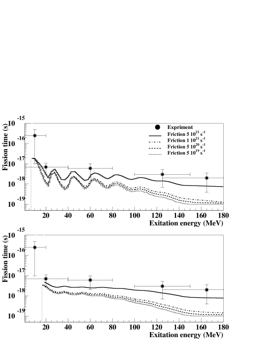
FIG. 3.: Fission time of ${}^{238}U$ as a function of the excitation energy. The upper panel represents the calculation done with a step of excitation energy of 3 MeV with angular momentum of the compound nucleus $J=1,5$ and $9\hbar$. The lower panel shows an averaging of the calculation on a range of 30 MeV. The curves represent the calculation done with various values of the friction factor $\beta$. The symbol represent the experimental data.

We see that the experimental data present no oscillation, but have very large error bars. The huge size of the error bars would be the main argument to explain the absence of oscillations. Actually, if we plot the same calculation as in the upper panel but averaged on a range of 30 MeV (range comparable to the mean value of the error bars) shown in the lower panel of the figure 4, we can see that the oscillations roughly disappear.

The agreement between the experimental data and the calculation are reasonably good. The experimental value and the calculation are all in agreement within a range of roughly one order of magnitude. The evolution of the calculated curves as a function of the friction parameter $\beta$ is rather strong when we go from $\beta=1~{}10^{21}s^{-1}$ to $\beta=5~{}10^{21}s^{-1}$ this is due to the Kramers factor (see equation (42)) as describe in the section 1. It seems that the friction value of $5~{}10^{21}s^{-1}$ is the best to reproduce experimental data. However, we have to be careful on some points to give definitive conclusion: information is missing on angular momentum distribution. The reliability of the conclusion could probably be improved by having more information on the distribution of angular momentum as a function of the excitation energy.

We should notice that in those calculations the value of the reduce friction coefficient $\beta$ that gives the best agreement with the data is $5~{}10^{21}s^{-1}$ and in the section IV A the value of $\beta$ is set to $5~{}10^{20}s^{-1}$. This difference in the suitable value of $\beta$ is a rather delicate problem which goes beyond the scope of this paper. Detailed analysis will be published elsewhere.

V Conclusion

The KEWPIE code has been designed as a disintegration code dedicated specifically to the study of superheavy elements. Its conception is based on the idea of minimising the number of free parameters. So the only free parameter that is adjusted in the calculation is the reduced friction coefficient $\beta$. We have shown that the results of the calculation with such a high level of constraint of only one adjustable parameter are rather successful. The quality of the agreement is as good as other evaporation codes that are including more adjustable parameters. The results of the calculation on the superheavy elements show that the shell correction energy is a key physical quantity for understanding and reproducing the residue cross sections.

The architecture of the program as a full cascade is an innovation which permits us to include the dynamics of the reaction. Thus, the evolution during the decay can be calculated. This time dependence permits to calculate fission time dynamically. The results of the calculations appear to be in quite a good agreement with the experimental data.

The KEWPIE program permits to study the disintegration of nucleus and to accommodate both a statistical and a dynamical frameworks. Moreover the way of programming allows us to implement new physical effects in the code without affecting the whole structure.

- [1] H. Bateman, Proc. Cambridge Phil. Soc. 16, 423 (1910)
- [2] D. Hilscher and H. Rossner, Ann. Phys. Fr. 17, 471 (1992)
- [3] Y. Abe, S. Ayik, P.G. Reinhard and E. Suraud, Phys. Rep. 275, 49 (1996)
- [4] A. Gavron, et al. Phys. Rev. C35, 579 (1987)
- [5] A.J. Cole, Statistical Models for Nuclear Decay, IoPP (2000).
- [6] Y. Abe et al., Prog. Theor. Phys. Suppl. 146, 104 (2002)
- [7] C. Shen, G. Kosenko and Y. Abe, Phys. Rev. C 66, 061602(R) (2002)
- [8] G. Kosenko et al., J. Nucl. and Radiochem. Sci 3 19 (2002)
- [9] S. Hassani and P. Grangé, Phys. Lett. 137B, 281 (1984)
- [10] V. Weisskopf, Phys. Rev. C52, 295 (1937)
- [11] W. Hauser and H. Feshbach, Phys. Rev. 87, 366 (1952)
- [12] N. Bohr and J.A. Wheeler, Phys. Rev. 56, 426 (1939)
- [13] D. L. Hill and J.A. Wheeler, Phys. Rev. 89, 1102 (193)
- [14] H.A. Kramers, Physica VII 4, 284 (1940)
- [15] J.M. Strutinski, Phys. Lett. 47, 121 (1973)
- [16] J.R. Grover and J. Gilat, Phys. Rev. 157, 802,814,823 (1967)
- [17] F. H. Ruddy, B. D. Pate and E. W. Vogt, Nucl. Phys. A127, 323 (1969)
- [18] P. Møller et al, Atomic Data Nucl. Data Tables 59, 185 (1995)
- [19] H. Koura et al., Nuc. Phys. A674, 47 (2000)
- [20] K.H. Schmidt W. Moraveck, Rep. Prog. Phys. 54, 949 (1991)
- [21] S. Cohen, F. Plasil and W.J. Swiatecki, Annal of physics 82, 557 (1974)
- [22] M. Dahlinger et al, Nucl. Phys. A 376, 94 (1982)
- [23] Bohr and Mottelson, Nuclear structure, vol. 1 Benjamin (1969)
- [24] Bohr and Mottelson, Nuclear structure, vol. 2 Benjamin (1969)
- [25] R.W. Hasse and W.D. Myers, Geometrical relationships of macroscopic nuclear physics, Springer-Verlag (1988)
- [26] J. Töke W.J. Swiatecki, Nuc. Phys. A372, 141 (1981)
- [27] A.V. Ignatyuk et al., Yad. Fiz. 21, 485 (1975)
- [28] M.A. Melkanoff, T.Sawada and J. Raynal, Meth. Comput. Phys. 6, 1 (1966)
- [29] Wilmore and Hogdson, Nuc. Phys. 55, 673 (1964)
- [30] F.D. Becchetti and G. W. Greenlees, Phys. Rev. 182, 1190 (1969)
- [31] T. Sikkeland et al., Phys. Rev. 172, 1232 (1968)
- [32] V.L. Mikheev et al., Yu. P.: At Energ 22, 90 (1967)
- [33] A.N. Andreyev et al., Z. Phys. A 345, 389 (1993)
- [34] J. Blocki and W.J. Swiatecki, Ann. Phys. 132, 53 (1981)
- [35] S. Bjornholm and W.J. Swiatecki, Nucl. Phys. A391, 471 (1982)
- [36] W. Reisdorf, J. Phys. G: Nuck. Part. 20, 1297 (1994)
- [37] W. Reisdorf, Z. Phys. A 300, 227 (1981)
- [38] H.W. Gäggeler et al., Nucl. Phys. A502, 501C (1989).
- [39] M. Morjean et al., Nucl. Phys. A630, 200 (1998)
- [40] I. Diozegi et al., Phys. Rev. C 46, 627 (1992)
- [41] K. Siwek-Wilcyńska et al., Phys. Rev. C 51, 2054 ( 1995)
- [42] T. Wada et al., Phys. Rev. Lett. 70, 3538(1993)
- [43] D.J. Hinde et al., Phys. Rev. C 45, 1229 (1992)
- [44] R. Butsh et al., Phys. Rev. C 44, 1515 (1991)