On Theoretical Problems in Synthesis of Superheavy Elements

Abstract

Towards precise predictions of residue cross sections of the superheavy elements, recent theoretical developments of reaction mechanisms are presented, together with the remaining problems which give rise to ambiguities in absolute values of cross sections predicted.

24.60.-k, 25.60.Pj, 25.70.-z, 25.70.Jj, 27.90.+b  A$\geq$220

1 Introduction

Predictions and structure studies of superheavy elements (SHE) have been made, since the establishment of the nuclear shell model[1]. Especially in the last decade, elaborate investigations have been performed of shell correction energy and thereby of a possible location of the superheavy island in the nuclear chart. Furthermore, not only about the center of the island, but also about stability properties of nearby nuclei have been being investigated, which is useful for the extension of the nuclear chart in heavy and superheavy elements[2]. On the other hand, studies of nuclear reaction mechanisms have not been developed so much, though so-called fusion-hindrance was experimentally found to exist in heavy ion fusions and inferred to be due to energy dissipation[3]. That is, there is no reliable theoretical framework which enables us to predict fusion probability of massive systems and thereby residue cross sections of SHE properly. Thus, which combination of incident ions is most promising and what incident energy is an optimum is not yet predicted theoretically. Therefore, the fusion experiments have been performed, based on systematics of data available so far[4].

Based on the reaction theory of the compound nucleus[5], residue cross sections are given as follows,

$$\sigma=\pi{\lambda\!\!\!^{-}}^{2}\Sigma(2J+1)\cdot P^{J}_{\mbox{\scriptsize fusion}}\cdot P^{J}_{\mbox{\scriptsize surv}},$$ (1)

where $\lambda\!\!\!^{-}$ is the wave length divided by $2\cdot\pi$ and $J$ the total angular momentum of the system. $P_{\mbox{\scriptsize fusion}}$ and $P_{\mbox{\scriptsize surv}}$ are fusion and survival probabilities, respectively. In the present paper, we discuss several difficult problems inherent in synthesis of the superheavy elements with brief explanations of a few progresses of our understanding, as well as attempts of realistic calculations.

2 Difficulties Characteristic in Synthesis of SHE

In order to obtain the fusion probability, we have to take into account possible mechanisms for the fusion-hindrance. Otherwise, calculated probabilities, and fusion cross sections would be unrealistic, as it is the case that one uses a transmission coefficient of an optical model or a barrier penetration factor as the fusion probability. As for possible origins of the hindrance, two mechanisms are proposed. One is dissipation of incident energy in the course of two-body collisions and thus probability for the system to overcome the Coulomb barrier is reduced[7]. The other one is dissipation of energy of collective motions of the amalgamated system which has to overcome a conditional saddle or a ridge line in order to reach the spherical shape, i.e., the compound nucleus[8]. Thus, the probability for reaching the spherical shape is also reduced. It is natural to consider that both exist. In other words, the fusion probability $P_{\mbox{\scriptsize fusion}}$ consists of two factors; the sticking probability $P_{\mbox{\scriptsize stick}}$ of two incident ions after overcoming the Coulomb barrier and the formation probability $P_{\mbox{\scriptsize form}}$ of the spherical shape after overcoming the conditional saddle point, starting from a pear-shaped configuration made by the sticking of the incident ions[9].

$$P^{J}_{\mbox{\scriptsize fusion}}=P^{J}_{\mbox{\scriptsize stick}}\cdot P^{J}_{\mbox{\scriptsize form}}.$$ (2)

Since the existence of the saddle point or the ridge line between a pear- shape made by the incident ions and the spherical shape is typical in very heavy systems, the latter mechanism would be indispensable for the fusion- hindrance observed in massive systems, though the former would also play a role (Note that in lighter heavy-ion systems the amalgamated shape is usually located inside the ridge line, so the system eventually slides down to the spherical shape with probability being equal to 1, once the incident ions stick to each other, though fluctuations to be discussed below may reduce it only slightly). In either mechanism, we have to describe a passing over a barrier under energy dissipation, which is not yet well understood theoretically[10] and thereby there is no useful formula ready for practical applications. This is quite contrast to a similar problem, i.e., to fission under dissipation, where a famous Kramers formula[11] for decay rate is known to well describe a process of a system inside a potential pocket leaking over the fission barrier. An essential difference is that in the latter the initial system is in the quasi-equilibrium in the pocket, while in the former the initial state is given by the condition of two incident ions with a given incident c.m.energy.

Recently, the present author and his collaborators have proposed a new analytic formula for the probability of passing over a parabolic barrier under frictional force. We have applied this formula to the problem of passing-over a conditional saddle point, and obtained a simple expression for so-called extra-push energy which provides a clear understanding of the fusion hindrance[12, 13]. This would be an important contribution to study of fusion mechanisms and is briefly recapitulated in section 3., but there still remains a difficulty in practice. The parabolic shape is usually a good approximation for barrier shapes, but in potential landscapes calculated with the liquid drop model (LDM) a pocket inside the saddle is very shallow in nuclei corresponding to the superheavy elements, as is easily expected from the fissility parameter $x_{f}$ being close to 1. Therefore, the potential is expected to be substantially asymmetric around the saddle, and moreover a system once passing over the saddle may return back with an appreciable probability due to the fluctuation associated with the friction. Of course, the probability for return-back to re-separation is reduced if the system is cooled down by neutron emissions and restores the shell correction energy which makes the pocket deeper.

For a quantitative prediction, those features should be taken into account properly, which is made by numerically solving a Langevin equation[14]. For a dynamical description of shape evolutions, we have to solve trajectories in a multi-dimensional space of shape parameterization with a realistic LDM potential, examples of which are discussed in section 5. But a time-dependent shell correction energy due to evaporation of neutrons is not yet taken into account in fusion processes. (Since time for fusion process is expected to be rather short, this would not cause a serious inaccuracy, but is properly done in the calculation of survival probability, as will be discussed in sections 6. and 7.) In the approaching phase of passing over the Coulomb barrier under friction, we have to take into account a dissipation of the orbital angular momentum as well as that of the kinetic energy of the radial motion, where a coupling between them is not described by a quadratic potential, as is discussed in section 4. Of course, there are many other effects which may play a role in the latter process, say, effects of deformations of incident ions, quantum tunneling effects etc., which are not yet fully investigated.

As for the survival probability, the statistical theory of decay is well established for obtaining a probability for the system to survive against fission and charged particle decay. But in practice there are ambiguities in the physical parameters, i.e., so-called level-density parameter $a$ and the shell damping energy $E_{d}$ which controls restoration of the shell correction energy by cooling. Especially, the latter is crucially important, because the restoring shell correction energy gives rise to an additional fission barrier effectively which controls survival probability, which is discussed qualitatively in section 6. and quantitatively in section 7. In addition, there are Kramers[11, 15] and collective enhancement factors[16] in fission decay widths to be taken into account. These are briefly discussed and examples of realistic calculations on ⁴⁸Ca+ actinide targets are presented which are made by employing a new statistical code KEWPIE[17] for the survival probabilities, in section 6.

3 Fusion Hindrance and Extra-Push Energy : Parabolic Barrier

We study a problem of obtaining a probability for passing over a potential barrier under a frictional force, which originates from interactions of the degree of freedom under investigation with a heat bath, i.e., with other degrees of freedom. Therefore, there should be a random force associated with the friction in accord with the dissipation-fluctuation theorem. If we approximate the barrier with an inverted parabolic shape, the equation of motion for a coordinate $q$ and its associate momentum $p$ is written as follows,

$$\frac{d}{dt}\left(\begin{array}[]{c}q\\ p\end{array}\right)=\left(\begin{array}[]{cc}0&1/m\\ m\omega^{2}&-\beta\end{array}\right)\left(\begin{array}[]{c}q\\ p\end{array}\right)+\left(\begin{array}[]{c}0\\ R\end{array}\right),$$ (3)

where $m$ denotes the inertia mass,and $\omega$ the curvature of the inverted parabola. $\beta$ is a reduced friction, i.e., the friction $\gamma$ divided by $m$, while $R$ is its associated random force. The random force is assumed to be Gaussian and satisfies the flowing properties,

$$\left<R(t)\right> = 0,$$ (4)

$$\left<R(t)\cdot R(t^{\prime})\right> = 2\cdot\gamma\cdot T\cdot\delta(t-t^{\prime}),$$

where $\left<\right>$ signifies an average over all the possible realizations and the last equation given in Eq. (4) with temperature $T$ of the heat bath expresses the dissipation-fluctuation theorem. Since the equation is linear, one can write down a general solution.

With this solution an general expression for a distribution function $W(q,p;t)$ at any later time t is calculated, starting with the following definition,

$$W(q,p;t)=\left<\delta\left(q-q(t)\right)\cdot\delta\left(p-p(t)\right)\right>_{\left\{R\right\}},$$ (5)

where $q(t)$ and $p(t)$ denote a general solution of Eq. (3) and is given by a linear combination of their initial value $q_{0}$ and $p_{0}$ with the coefficients including parameters $\beta$ and $\omega$. $\left<\right>_{\left\{R\right\}}$ again denotes the average over all the possible realizations of $R(t)$. Using the path integral technique, we can perform the averaging and obtain the distribution function of the system as a Gaussian distribution around the mean trajectory $\left(\left<q(t)\right>,\left<p(t)\right>\right)$[12]. Then, a probability for passing over the barrier is calculated by integrating over the whole $p$-space and the half $q$-space, and then by taking the limit of time $t$ to the infinity,

$$P_{\mbox{\scriptsize form}}=\frac{1}{2}\mbox{erfc}\left[\sqrt{\frac{\sqrt{x^{2}+1}+x}{2x}}\left\{\sqrt{\frac{B}{T}}-\frac{1}{\sqrt{x^{2}+1}+x}\sqrt{\frac{K}{T}}\right\}\right],$$ (6)

where $x$ denotes $\beta$ divided by $2\cdot\omega$. $K$ and $B$ denote the initial kinetic energy $p_{0}^{2}/2\mu$ and the barrier height measured from the initial potential energy $\mu\cdot\omega^{2}\cdot q_{0}^{2}/2$, respectively.

In order for the probability to be 1/2, the argument of the error function should be equal to zero, which means that the mean trajectory just reaches at the top of the barrier overcoming the friction. Then, the necessary critical kinetic energy $K_{c}$ is given as

$$K_{c}=\left(\sqrt{x^{2}+1}+x\right)^{2}\cdot B,$$ (7)

where we can see that in the case of no friction, i.e., of $x$ being equal to zero, $K_{c}=B$, which is trivial. It clearly shows that $K_{c}$ is much larger than $B$ under the frictional force. If we estimate the first factor in Eq. (7), assuming One-Body Wall-and-Window formula (OBM[18]) for the friction $\gamma$, we obtain about 10, depending on a reasonable choice of values for the inertia mass and the curvature of the potential calculated with LDM. This gives a simple formula for the extra-push energy, though we should be careful in a comparison with experimental data about effective one-dimensional quantities for $B$, $\mu$, $\omega$ and Coulomb barrier heights of entrance channel etc.

Another interesting formula is obtained, which is very useful for synthesis of SHE. Residue cross sections are extremely small in SHE, i.e., we are facing with the situation where fusion probability is very small. This suggests in our present formulation that the mean trajectory does not reach the top of the barrier, even is far before the top, which means that the argument of the error function of Eq. (6) is very large. Then, employing an asymptotic expansion of the error function, we can obtain a simple approximate formula for the formation probability $P_{\mbox{\scriptsize form}}$[13],

$$P_{\mbox{\scriptsize form}}\cong\frac{1}{2}\frac{1}{\sqrt{\pi}}\left[\sqrt{\frac{\sqrt{x^{2}+1}+x}{2x}}\left\{\sqrt{\frac{B}{T}}-\frac{1}{\sqrt{x^{2}+1}+x}\sqrt{\frac{K}{T}}\right\}\right]^{-1}$$ (8)

$$\cdot\exp\left[\sqrt{\frac{\sqrt{x^{2}+1}+x}{2x}}\left\{\sqrt{\frac{B}{T}}-\frac{1}{\sqrt{x^{2}+1}+x}\sqrt{\frac{K}{T}}\right\}\right],$$

where it is interesting to note that there is a factor very similar to Arrhenius factor which is typical in thermal activation processes such as nuclear fission, neutron evaporation, thermal electron emission from metal, etc. The exact Arrhenius factor is obtained in case of a complete damping of the relative motion in the approaching phase, as follows. As will be shown in the next section, a distribution of the radial momentum at the contact point is approximately expressed by a Gaussian as a results of two-body collision processes and thus, the formation probability is obtained by a convolution over initial momentum $p_{0}$, which results again in an error function of Eq. (6) with K being replaced with the average value $\bar{K}$ and with the associated variance. In case of completely damping, $\bar{K}$ is equal to zero, and the variance is equal to the temperature. Accordingly, the corresponding asymptotic expansion gives the exact Arrhenius factor.

$$P_{\mbox{\scriptsize form}}\cong\frac{1}{2}\frac{1}{\sqrt{\pi}}\sqrt{\frac{T}{B}}\exp\left[-\frac{B}{T}\right]$$ (9)

Since fusion is inverse to fission in reaction directions, one could call this as an “inverse Kramers formula[19]”. But we should be careful that in the thermal activation processes the factor appears in decay rate or in emission rate per unit time, while in the present case it appears in the transition probability, i.e., time-integrated quantity. Anyhow, a physical meaning of the factor as well as of the pre-exponential factor are yet to be understood.

For actual fusion reactions, one-dimensional treatment is obviously an over-simplification, which is readily understood by considering a mass-asymmetric entrance channel. In addition, neck formation etc. would come into play. It is worth to notice that even in such situations, i.e., in multi-dimensional problems, we can derive the same type of formula as Eq. (6), starting with an assumption of a quadratic potential generalized to a multi-dimension. That indicates that we can define an effective one-dimensional model. Thus, the qualitative understandings obtained above with the schematic one-dimensional model are considered to be useful, with the barrier height etc. being considered to be effective quantities.

4 Approaching Phase ; Passing-Over Coulomb Barrier under Friction

One could apply the formula obtained in the previous section to passing-over Coulomb barrier, approximating again the barrier as an inverted parabola. There, however, is another problem, as stated in section 2. In the approaching phase,dissipation of the orbital angular momentum comes into play, coupled with the radial motion. For the problem, the most simple and readily applicable model is the surface friction model (SFM), proposed by Gross and Kalinowski[6] in order to explain so-called Deep-Inelastic Collisions.

Below, we reformulate it, starting with a general framework of Ref. [20] which includes so-called rolling friction. Starting with intrinsic spins of the incident ions, $L_{1}$ and $L_{2}$, respectively, we introduce the following variables,

$$L^{+} = L_{1}+L_{2}=L_{0}-L(t)$$ (10)

$$L^{-} = \left(C_{1}L_{2}-C_{2}L_{1}\right)/C_{1}+C_{2},$$

where $L_{0}$ denotes an incident orbital angular momentum and $C_{i}$, $i$ being 1 or 2, is an effective ion radius defined as follows,

$$C_{i}=R_{i}\left(1-\left(b/R_{i}\right)^{2}\right),$$ (11)

where $b=1\mbox{fm}$ and $R_{i}=1.28\cdot A^{1/3}_{i}-0.76+0.8\cdot A^{-1/3}_{i}$ with $A_{i}$ being the mass number of $i$-th ion. Then, a Langevin equation for two-body collisions is written as

$$\frac{dr}{dt} = \frac{1}{\mu}p$$ (12)

$$\frac{dp}{dt} = -\frac{dV}{dr}-\beta_{r}\cdot p+\theta_{r}\cdot\omega_{r}(t)$$ (13)

$$\frac{d}{dt}\left(\begin{array}[]{@{}c@{}}L\\ L^{-}\end{array}\right) = \left(\begin{array}[]{@{}cc@{}}\beta_{11}&\beta_{12}\\ \beta_{21}&\beta_{22}\end{array}\right)\left(\begin{array}[]{@{}c@{}}L\\ L^{-}\end{array}\right)+\left(\begin{array}[]{@{}c@{}}\tilde{\beta_{11}}\\ \beta_{21}\end{array}\right)\cdot L_{0}+\left(\begin{array}[]{@{}cc@{}}\theta_{11}&\theta_{12}\\ \theta_{21}&\theta_{22}\end{array}\right)\left(\begin{array}[]{@{}c@{}}\omega_{1}\\ \omega_{2}\end{array}\right),$$ (26)

where $\mu$ is equal to the reduced mass of the entrance channel, and $V$ denotes a sum of the Coulomb $V_{c}$ and the nuclear $V_{n}$ potentials with the rotational energy given by the orbital angular momentum $L$. The friction tensor $\beta_{ij}$ and $\beta_{r}$ are given below,

$$\beta_{r} = C_{r}\Psi(r)/\mu$$ (27)

$$\left(\begin{array}[]{@{}c@{\,}c@{}}\beta_{11}&\beta_{12}\\ \beta_{21}&\beta_{22}\end{array}\right) = \left(\begin{array}[]{@{}c@{\,}c@{}}-\Psi(r)\cdot C_{T}\cdot\left[\frac{1}{\mu}+\frac{r^{2}}{\left(C_{1}+C_{2}\right)^{2}}\cdot\frac{C^{2}_{1}J_{2}+C^{2}_{2}J_{1}}{J_{1}\cdot J_{2}}\right]&-\Psi(r)\cdot C_{T}\left[\frac{r^{2}}{C_{1}+C_{2}}\cdot\frac{C_{1}J_{2}-C_{2}J_{1}}{J_{1}\cdot J_{2}}\right]\\ -\Psi(r)\cdot C_{\mbox{\scriptsize roll}}\cdot g^{2}\left[\frac{1}{C_{1}+C_{2}}\frac{C_{1}J_{2}-C_{2}J_{1}}{J_{1}\cdot J_{2}}\right]&-\Psi(r)\cdot C_{\mbox{\scriptsize roll}}\cdot g^{2}\cdot\frac{J_{1}+J_{2}}{J_{1}\cdot J_{2}}\end{array}\right),$$ (32)

where $\Psi(r)$ is a form factor specified below, and $C_{T}$ and $C_{\mbox{\scriptsize roll}}$ denote strengths for tangential and rolling frictions, respectively, In addition, a parameter $g$ is introduced for describing a effective depth of the rolling friction, which is taken to be 1.0fm. $J_{i}$, $i$ being 1 and 2, are the rigid moment of inertia of the incident ions which are assumed to be spherical. Then, the strengths $\theta_{r}$ and $\theta_{ij}$ are adjusted to satisfy the dissipation-fluctuation theorem with the friction tensor $\beta_{r}$ and $\beta_{ij}$. The coefficient $\tilde{\beta}_{11}$ is given by $\beta_{11}-\Psi(r)\cdot C_{T}/\mu$. Langevin forces are given by $\omega_{i}$, $i$ being $r$, 1 and 2 which denote Gaussian random numbers and are assumed to have the following properties,

$$\left<\omega_{i}\right>=0,\left<\omega_{i}(t)\omega_{j}(t^{\prime})\right>=2\cdot\delta_{ij}\cdot\delta(t-t^{\prime})$$ (33)

If one wants to introduce deformations of the ions, one has to introduce additional degrees of freedom which describe their orientations. If we assume that the rolling friction is very weak compared with the others, we take $C_{\mbox{\scriptsize roll}}$ to be zero. Then, $dL-/dt=0$, and $L_{-}=\mbox{constant}=L_{-}(-\infty)=0$. The equation for the orbital angular momentum is rewritten simply as follows,

$$\frac{dL}{dt}=-K_{\Phi}/\mu\cdot\left(L-L_{st}\right)+\theta_{11}\cdot\omega_{1},$$ (34)

where the effective friction $K_{\phi}$ and the limiting angular momentum $L_{st}$ are given as

$$K_{\phi} = C_{T}\cdot\left[1+\frac{\mu r^{2}}{(C_{1}+C_{2})^{2}}\cdot\left(\frac{C^{2}_{1}}{J_{1}}+\frac{C^{2}_{2}}{J_{2}}\right)\right]\cdot\Psi(r)$$ (35)

$$L_{st} = \left(\frac{C^{2}_{1}}{J}+\frac{C^{2}_{2}}{J}\right)\cdot\mu r^{2}/\left[\left(C_{1}+C_{2}\right)^{2}+\left(\frac{C^{2}_{1}}{J_{1}}\frac{C^{2}_{2}}{J_{2}}\cdot\mu r^{2}\right)\right]$$

If we approximate $R_{i}\cong C_{i}$,

$$K_{\phi} \cong \frac{7}{2}C_{T}\Psi(r),$$ (36)

$$L_{st} = \frac{5}{7}L_{0}.$$

$L_{st}$ is so-called rolling limit, while one could obtain the sticking limit if one takes the limit that the drift part of the r.h.s. of Eq. (15) is equal to null vector, as discussed in Ref. [21]. Together with $K_{r}=\mu\beta_{r}=C_{r}\cdot\Psi(r)$, Eqs. (12), (13) and (17) just correspond to SFM. The correspondence is precised by giving the following relation of the friction forces,

$$\Psi(r)=\left(\frac{dV_{N}}{d_{r}}\right)^{2},\;\;\;K^{0}_{\phi}=\frac{7}{2}C_{T}=0.01,\;\;\;K^{0}_{r}=C_{r}=4,$$ (37)

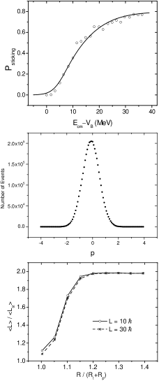
Figure 1: Results of SFM calculations for ⁴⁸Ca+²⁴⁴Pu system. The top panel shows the sticking probability $P_{\mbox{\scriptsize stick}}$ as a function of incident energy relative to the Coulomb barrier. The middle panel shows the distribution of the radial momentum at the contact point, where $P$ is given in unit of 10^-21sec$\cdot$MeV/fm. The bottom panel shows the orbital angular momentum divided by the limit $L_{st}$ as a function of relative distance.

where the numerical values are given in unit of 10^-23s/MeV. The dissipation-fluctuation theorem is satisfied by the equations: $\theta^{2}_{r}=K_{r}\cdot T_{A}$ and $\theta^{2}_{11}=r^{2}\cdot K_{\phi}\cdot T_{A}$ with $T_{A}\equiv T_{A}(t)$ being temperature of the colliding system in the approaching phase. Examples of numerical solutions with the proximity model and with SFM are given in Ref. [22]. Generally speaking, the former is much weaker than the latter, but for the moment we cannot draw a definite conclusion on which one is correct or more realistic. The former neglects frictional force stemming from strong inelastic excitations etc., while the latter does a rolling friction.

We have applied SFM to superheavy systems, such as ⁴⁸Ca + actinide targets. As an example, we discuss results on ⁴⁸Ca + ²⁴⁴Pu system in detail. The top panel of Fig. 1 shows probability $P_{\mbox{\scriptsize stick}}$ for the entrance system to reach the contact point, i.e., the relative distance being equal to a sum of the half density radii of the incident ions as a function of $E_{\mbox{\scriptsize c.m.}}$ relative to the barrier height. If there is no friction, it should be always equal to 1 above the barrier height (Below the barrier, it is equal to zero, since the equation is classical.). But the results are not like that. It starts with an extremely small value at the barrier height energy and slowly increases to reach 1/2 about 12 MeV above the barrier, which would explain a part of the extra-push. More interesting is that a distribution of the radial momentum calculated at the contact point is found to be approximately of a Gaussian one with its average value being almost exactly equal to zero as shown in the middle panel of Fig. 1, which indicates that the relative motion is completely damped at the contact point. In fact, the average orbital angular momentum also approaches to the dissipation limit at the contact point, which is shown in the bottom panel of Fig. 1. This is also the case for other actinide targets, say, ²⁴⁸Cm and ²⁵²Cf.

In brief, the analyses of the approaching phase provide us with sticking probability $P_{\mbox{\scriptsize stick}}(E_{\mbox{\scriptsize c.m.}})$ as well as with information of the amalgamated system, with which we can start to solve a Langevin equation for shape evolutions and then, can obtain formation probability $P_{\mbox{\scriptsize form}}$. This means that we treat the two-body collision processes and shape evolutions of the united system consistently.

5 Realistic Calculations of $P_{\mbox{\scriptsize form}}$ and Fusion Cross sections

In order to describe shape evolutions starting from the pear-shape configuration of the amalgamated system to the spherical shape, at least, three parameters, say, distance between two mass centers $R$, mass asymmetry $\alpha$, and neck parameter $\epsilon$ in the Two-Center Parameterization[23]. With OBM[18], the friction for the neck degree of the freedom is much stronger than the others and thus its motion is considered to be much slower than the other twos. Then, we expect that two variables could describe the formation dynamics reasonably well, with the neck parameter $\epsilon$ freezed. We again employ a classical dissipation- fluctuation description, though quantum effects, such as a tunneling effect, might play a significant role in passing over the saddle.

A multi-dimensional Langevin equation is written as usual[24],

$$\frac{dq_{i}}{dt} = (m^{-1})_{ij}\cdot p_{j}$$ (38)

$$\frac{dp_{i}}{dt} =- \frac{\partial U}{\partial q_{i}}-\frac{1}{2}\frac{\partial}{\partial q_{i}}(m^{-1})_{jk}\cdot p_{j}\cdot p_{{}_{\mbox{\scriptsize R}}}-\gamma_{ij}\cdot(m^{-1})_{jk}\cdot p_{k}+g_{ij}\cdot\Gamma_{j},$$

where $q_{i}$, $i$ being 1 or 2, specifies $R$, or $\alpha$, and summations are implicitly assumed over the repeated indices. The inertia mass tensor $m_{ij}$ is calculated by Werner-Wheeler approximation[25] and the friction tensor $\gamma_{ij}$ by OBM as functions of the variables $R$ and $\alpha$. The potential $U$ is given also by the macroscopic LDM energy. In case of a finite angular momentum, it should include the rotational energy calculated with the rigid moment of inertia. The random force in the r.h.s. of Eq. (21) is assumed to be Gaussian and is expressed with a Gaussian number $\Gamma_{i}$ and a strength tensor $g_{ij}$ which are assumed to satisfy the following properties,

$$\left<\Gamma_{i}(t)\right> = 0$$ (39)

$$\left<\Gamma_{i}(t)\cdot\Gamma_{j}(t^{\prime})\right> = 2\cdot\delta_{ij}\cdot\delta(t-t^{\prime})c$$

$$g_{ik}g_{jk} = \gamma_{ij}\cdot T,$$

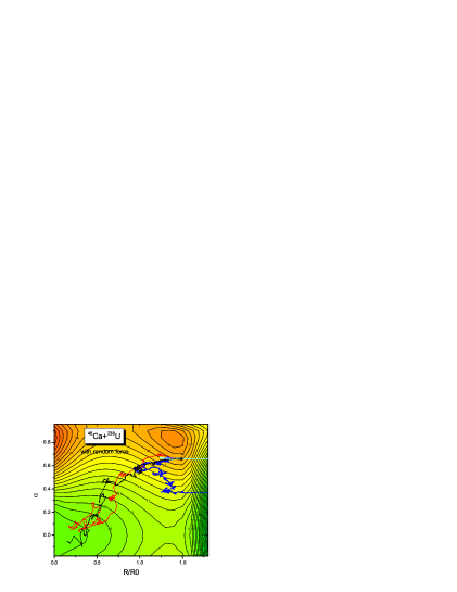
Figure 2: Examples of trajectories in two-dimensional space of the relative distance $R$ divided by the radius of the sphere of the total system $R_{0}$ and the mass-asymmetry $\alpha$ for ⁴⁸Ca+²³⁸U system. Initial momenta are taken to be zero, but Langevin forces are calculated with the temperature given by the excitation energy of 70MeV.

where $\left<\right>$ denotes an average over all the possible realizations. The last equation expresses the dissipation-fluctuation theorem. In order to obtain a formation probability, i.e., a probability for the system to overcome the conditional saddle point or the ridge line, we have to calculate a large number of trajectories.

Examples are shown in Fig. 2, for ⁴⁸Ca-²³⁸U system with zero initial radial momentum but with the temperature corresponding to the excitation energy 70MeV, starting at the contact configuration. It is seen that some trajectories go into the spherical configuration and its around, while the others go back to re-separation. The formers consist a formation probability, while the latters do quasi-fission components which are to be carefully analysed in a future, including deformations of nascent fragments, mass drifts etc. before scission.

Formation probabilities calculated with $\epsilon$ being 0.8 are shown in the upper panel of Fig. 3, for ⁴⁸Ca-²³⁸U system. And fusion probabilities calculated by Eq. (2), i.e., obtained by combining with the sticking probabilities obtained by SFM, are shown in the lower panel of Fig. 3 for the total angular momenta of the system $J=0$ and 30. Then, excitation functions of fusion cross sections are calculated according to the following formula,

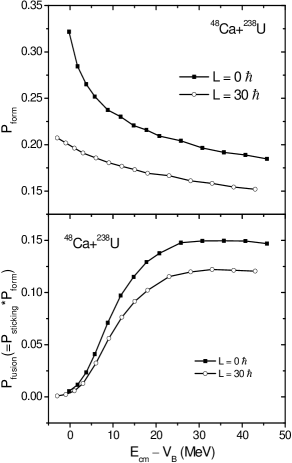
Figure 3: The upper panel shows the formation probability $P_{\mbox{\scriptsize form}}$ calculated for the total spin $J=0$ and 30 cases of ⁴⁸Ca+²³⁸U system, as a function of incident energy relative to the Coulomb barrier. The lower panel shows the corresponding fusion probability $P_{\mbox{\scriptsize fusion}}$ calculated together with $P_{\mbox{\scriptsize stick}}$ by SFM.

$$\sigma_{\mbox{\scriptsize fusion}}=\pi{\lambda\!\!\!^{-}}^{2}\Sigma(2J+1)\cdot P_{\mbox{\scriptsize fusion}}.$$ (40)

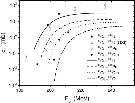
Figure 4: Calculated fusion excitation functions are shown for ⁴⁸Ca+²³⁸U, +²⁴⁴Pu, +²⁴⁸Cm, and +²⁵²Cf systems, together with the available experimental data from GSI[26] and Dubna[27].

The results for ⁴⁸Ca + actinide target systems are shown in Fig. 4, compared with the available experimental data obtained at GSI[26] and Dubna[27]. It is surprising that the calculations reproduce the experimental data very well, not only their absolute values, but also their energy dependence, systematically over three systems. A prediction is made for ${}^{252}C_{f}$ target case, which should be verified by experiment.

6 Survival Probability

The survival probability $P_{\mbox{\scriptsize surv}}$ is a probability for the compound system to survive against fission decay and charged particle emission. We first discuss the characteristic features qualitatively and then present examples of realistic calculations made by a new statistical code KEWPIE[17] in the next section. Since decay widths for the latters are small compared with those for the former and neutron emission, the total decay width is approximately given by $\Gamma_{f}+\Gamma_{n}$, and then the survival probability is given approximately by

$$P_{\mbox{\scriptsize surv}}\cong\Gamma_{n}/\left(\Gamma_{f}+\Gamma_{n}\right)\cong\Gamma_{n}/\Gamma_{f},$$ (41)

where $\Gamma_{f}$ and $\Gamma_{n}$ denote fission decay and neutron emission widths, given by Bohr-Wheeler[28] and Weisskopf[29] formulae, respectively. Of course, if intrinsic excitation energy $E^{*}$ is large enough for emissions of more than one neutron, the expression of Eq. (24) is repeatedly used in multiplication. In SHE, $\Gamma_{f}\gg\Gamma_{n}$, so the second equation approximately holds in superheavy nuclei generally except cases with very large shell correction energies, which is easily seen by their approximate expressions,

$$\Gamma_{n}\simeq e^{-B_{n}/T},\;\;\;\Gamma_{f}\simeq e^{-B_{f}/T},$$ (42)

then the probability is given by

$$P_{\mbox{\scriptsize surv}}\simeq e^{-\left(B_{n}-B_{f}\right)/T},$$ (43)

where $B_{f}$ and $B_{n}$ denote fission barrier height and neutron separation energy, respectively. And $B_{f}$ is almost equal to minus of the shell correction energy, because macroscopic fission barriers, i.e., LDM fission barrier $B_{f}^{\mbox{\scriptsize LDM}}$ is very small and is nearly equal to zero for SHE, due to the fact that the fissility parameter $x_{f}$ is close to 1.

It is worth to consider how an excitation-energy dependence of the shell correction energy comes into play. As is expected, absolute values of the shell correction energy are reduced by excitation, so in the beginning of decay process. This is well taken into account by Ignatyuk’s prescription[30] of excitation-energy dependence of the level density parameter of the spherical shape, i.e., for neutron emission,

$$a_{n} = \bar{a}_{n}\cdot\left[1+f(E^{*})\cdot\delta E/E^{*}\right],$$ (44)

$$f(E) = 1-\exp\left[-E^{*}/E_{d}\right],$$

where $\bar{a}_{n}$ is an asymptotic level density parameter in high excitation, and $E^{*}$ intrinsic excitation energy of the compound nucleus. $\delta E$ and $E_{d}$ denote shell correction energy of the ground state and so-called shell damping parameter, respectively. The parameter $E_{d}$ is obtained to be about 18 MeV by calculating excitation energy dependence of the free energy with a single particle model. With Eq. (27), the fission width is approximately given as follows,

$$\Gamma_{f} \cong e^{-B_{\mbox{\scriptsize eff}}/T},$$ (45)

$$B_{\mbox{\scriptsize eff}} = B_{f}+f(E^{*})\cdot\delta E.$$

Then, asymptotic behaviors for $E^{*}\ll E_{d}$ and $E^{*}\gg E_{d}$ become as follows respectively,

$$B_{\mbox{\scriptsize eff}}\cong B_{f}+E^{*}\cdot\delta E/E_{d}\rightarrow B_{f},\; E^{*}\ll E_{d},$$ (46)

$$\cong B_{f}+\delta E\rightarrow B_{f}^{\mbox{\scriptsize LDM}},\;\;\;\;\;\;\;\;\; E^{*}\gg E_{d},$$

where $B_{f}=B_{f}^{\mbox{\scriptsize LDM}}-\delta E$ denotes the fission barrier height of the ground state. As is seen from the above arguments, the survival probability $P_{\mbox{\scriptsize surv}}$ is crucially determined by absolute values of the shell correction energy!! Remaining ambiguities are Kramers[11, 15] and collective enhancement[16] factors. The former takes into account an effect of friction force acting on the fissioning degree of freedom, and is given by

$$K_{f}=\sqrt{x^{2}+1}-x.$$ (47)

This is always smaller than 1 and is approximately equal to $1/x$ in case of large $x$. The collective enhancement factor takes into account a difference between collective level densities at the spherical shape and the saddle point shape. Since the saddle point shape of SHE is determined by shape dependence of the shell correction energy, no simple formula is available. It should be worth to notice here that so-called Strutinski correction factor[31] for Bohr-Wheeler formula $\hbar\cdot\omega/T$ can be considered to be a part of the collective enhancement factor, i.e., the part from the fissioning collective degree of freedom, though the main part of the enhancement is expected to be that of the rotational degrees of freedom.

7 Preliminary Results of Residue Cross Sections

In order to make realistic calculation of the survival probability we have made a new statistical code KEWPIE (Kyoto Evaporation Width calculation Program with tIme Evolution)[17]. This program treats both the production of residue as a function of the time and the final residue production. In the present case we will only consider the amount of nuclei remaining at the end of the disintegration cascade. Detailed formalism and the computer code will be published elsewhere.

This program includes the main features required in the section 6. However in this code the evaporation width of particle is calculated more accurately in the Hauser-Feshbach formalism [32]. Moreover the evaporation of protons, alphas and gammas are included in the program. Calculation of fission width is done according to Bohr-Wheeler formula with the transmission coefficient by Hill and Wheeler[33] and with Strutinski correction factor. The fission barrier $B_{f}^{LDM}$ is that of the empirical formula given for heavy elements by K.H. Schmidt et al. in reference [34].

The level density parameters $\bar{a}_{n}$ and $a_{f}$ are calculated with Töke and Swiatecki formula[35] by taking into account of shapes of the ground state and the saddle point. At the ground state the shape of the nucleus is assume to be spherical and we take into account the shell correction effect with the Ignatyuk prescription [30] with $E_{d}=18$ MeV as given in Eq. (27). At saddle point, deformation is evaluated by the Hasse and Myers formula [36] and no shell correction effect are taken into account.

Figure 5: Residue cross sections calculated by the statistical code KEWPIE are shown for ⁴⁸Ca+²⁰⁸Pb, compared with the experimental data[38].

Figure 6: Calculated residue cross sections are shown for ⁴⁸Ca+²⁴⁴Pu system, together with Dubna data[39]. Details on the parameters are given in the text.

The KEWPIE calculation has few free parameters, the scaling factor of the shell correction taken from Møller et al.’s table[2] and the parameters of Kramer factor $K_{f}$. The latter is calculated with $\hbar\omega=1$ MeV and a friction factor $\beta=5\times 10^{20}sec^{-1}$.

For ⁴⁸Ca+²⁰⁸Pb system, fusion probabilities are calculated with the proximity potential[37], because no fusion hindrance is observed there. With the parameters fixed, we calculate $xn$ residue cross sectoins, whose results are shown in the Fig. 5. The experimental cross sections[38] are seen to be well reproduced, which appears to guarantee the code KEWPIE.

For ⁴⁸Ca+${}^{244}Pu$ reaction, we use fusion probabilities calculated according to Eq. (2) with the realistic calculations of $P_{\mbox{\scriptsize form}}$ given in section 5. As discussed in section 6, the crucial parameter in the survival probability $P_{\mbox{\scriptsize surv}}$ is the shell correction energy. The scaling factor of $2/3$ or even smaller has turned out to be necessary to the shell correction energies of P. Møller et al. in order to be consistent with the data[39], as is shown on Fig. 6. As theoretical values of the shell correction energy are very different from one model to another, more precise investigations are desired. We are now studying the reactions of ⁴⁸Ca + actinide targets, using several predictions of the shell correction energy, which could be very informative on the models of nuclear structure for heavy and superheavy nuclei.

Acknowldgements

Y. Abe acknowledges long-standing fruitful collaborations with T. Wada, D. Boilley, C.W. Shen, G. Kosenko and B. Giraud, with the results of which the present contribution is mostly written. B. Bouriquet thanks the supports for the post-doctoral position provided by JSPS which gives him an opportunity to work at Yukawa Institute for Theoretical Physics, Kyoto University. This work is partially supported by the Grant-in-Aids of JSPS (no. 1340278).

References

- [1] M.G. Mayer and J.H.D. Jensen, Elementary Theory of Nuclear Shell Structure, 1955, Wiley, New York.
-
[2]
R. Smolanczuk et al., Phys. Rev. C52, 1871
(1995),
Z. Patyk and A. Sobiczewski, Nucl. Phys. A533, 132 (1991),
P. Møller et al., Atomic Data and Nuclear Data Tables 59, 185 (1995),
P.G. Reinhard and H. Flocard, Nucl. Phys. A584, 467 (1995),
M. Bender et al., Eur. Phys. J. A7, 467 (2000). -
[3]
A.B. Quint et al., Z. Phys. A346, 119
(1993),
K.-H. Schmidt and W. Morawek, Rep. Prog. Phys. 54, 949 (1991),
W. Reisdorf, J. Phys. G20, 1297 (1994). -
[4]
S. Hofmann and G. Münzenberg, Rev. Mod. Phys.
72, 733 (2000),
P. Armbruster, Annu. Rev. Nucl. Part. Sci. 50, 411 (2000). - [5] N. Bohr, Nature 137, 344 (1936).
- [6] D.H.E. Gross and H. Kalinowski, Phys. Rept. 45, 175 (1978).
- [7] P. Fröbrich et al., Nucl. Phys. A406, 557 (1983).
- [8] W.J. Swiatecki, Physica Scripta 24, 113 (1981).
- [9] C.W. Shen et al., to appear in Rapid Comm. of Phys. Rev. C.
-
[10]
H. Hofmann and R. Samhammer, Z. Phys. A322, 157
(1985),
N. Takigawa and S. Ayik, private communication. - [11] H.A. Kramers, Physica VII 4, 284 (1940).
- [12] Y. Abe et al., Phys. Rev E61, 1125 (2000).
- [13] Y. Abe et al., Prog. Theor. Phys. Suppl., to appear.
- [14] Y. Abe et al., J. de Phys. 47, C4-329 (1986).
- [15] Y. Abe et al., Phys. Rept. 275, Nos. 2 and 3 (1996).
-
[16]
A.R. Junghaus et al., Nucl. Phys. A629, 635
(1998),
G. Hansen and A.S. Jensen, Nucl. Phys. A406, 236 (1983). - [17] B. Bouriquet et al., publication under preparation.
- [18] J. Blocki et al., Ann. Phys. (NY) 113, 330 (1978).
- [19] D. Boilley et al., publication under preparation.
-
[20]
C.F. Tsang, Physica Scripta 10A, 90 (1974),
D. Bangert and H. Freiesleben, Nucl. Phys. A340, 205 (1980). - [21] R. Bass, Nuclear Reaction with Heavy Ions (Springer-Verlag, Berlin, 1980) Chapt. 6.
- [22] G. Kosenko et al., J. Nucl. and Radiochem. Sci. 3, 19 (2002).
-
[23]
A. Iwamoto et al., Prog. Theor. Phys. 55,
115 (1976),
K. Sato et al., Z. Phys. A290, 145 (1979). - [24] T. Wada et al., Phys. Rev. Lett. 70, 3538 (1993).
- [25] K.T.R. Davies et al., Phys. Rev. C13, 2385 (1976).
- [26] W.Q. Shen et al., Phys. Rev. 36, 115 (1987).
- [27] M.G. Itkis et al., Il Nuovo Cimento 111A, 783 (1998).
- [28] N. Bohr and J.A. Wheeler, Phys. Rev. 56, 426 (1939).
- [29] V. Weisskopf, Phys. Rev. 52, 295 (1937).
- [30] A.V. Ignatyuk et al., Sov. J. Nucl. Phys. 21, 255 (1975).
- [31] V.M. Strutinski, Phys. Lett. B47, 121 (1973).
- [32] W. Hauser and H. Feshbach, Phys. Rev. 87, 366 (1952).
- [33] D. L. Hill and J.A. Wheeler, Phys. Rev. 89, 1102 (1953).
- [34] M. Dahlinger et al., Nucl. Phys. A376, 94 (1982).
- [35] J. Töke and W.J. Swiatecki, Nuc. Phys. A372, 141 (1981).
- [36] R.W. Hasse and W.D. Myers, Geometrical relationships of macroscopic nuclear physics Springer-Verlag (1988).
- [37] J. Blocki and W.J. Swiatecki, Ann. Phys. 132, 53 (1981).
- [38] H.W. Gäggeler et al., Nucl. Phys. A502, 501C (1989).
- [39] Yu. Oganessian et al., Phys. Rev. Lett. 83, 3154 (1999).