Next Generation Relativistic Models

1 Introduction

The current generation of covariant mean-field models has had many successes in calculations of bulk observables for medium to heavy nuclei, but there remain many open questions RING96 ; SEROT97 . New challenges are confronted when trying to systematically extend these models to reliably address nuclear structure physics away from the line of stability. In this lecture, we discuss a framework for the next generation of relativistic models that can address these questions and challenges. We interpret nuclear mean-field approaches as approximate implementations of Kohn-Sham density functional theory (DFT), which is widely used in condensed matter and quantum chemistry applications KOHN65 ; DREIZLER90 . We look to effective field theory (EFT) for a systematic approach to low-energy nuclear physics that can provide the framework for nuclear DFT FURNSTAHL00 .

We start with the key principle underlying any effective low-energy model and then describe how EFT’s exploit it to systematically remove model dependence from calculations of low-energy observables. Chiral EFT for few nucleon systems is maturing rapidly and serves as a prototype for nuclear structure EFT. The immediate question is: why consider a relativistic EFT for nuclei? We show how the EFT interpretation of the many-body problem clarifies the role of the “Dirac sea” in relativistic mean-field calculations of ground states and collective excited states (relativistic RPA). Next, the strengths of EFT-motivated power counting for nuclear energy functionals is shown by the analysis of neutron skins in relativistic models, which also reveals weaknesses in current functionals. Finally, we propose a formalism for constructing improved covariant functionals based on EFT/DFT. We illustrate the basic ideas using recent work on deriving systematic Kohn-Sham functionals for cold atomic gases, which exhibit the sort of power counting and order-by-order improvement in the calculation of observables that we seek for nuclear functionals.

2 Low-Energy Effective Theories of QCD

If a system is probed with wavelengths small compared to the size of characteristic sub-structure, then details of that substructure are resolved and must be included explicitly (e.g., see Fig. 2 for a nucleus). On the other hand, a general principle of any effective low-energy theory is that if a system is probed or interacts at low energies, resolution is also low, and what happens at short distances or in high-energy intermediate states is not resolved LEPAGE ; CROSSING . In this case, it is easier and more efficient to use low-energy degrees of freedom for low-energy processes (see Fig. 2). The short-distance structure can be replaced by something simpler (and wrong at short distances!) without distorting low-energy observables. This principle is implicit in conventional nonrelativistic nuclear phenomenology with cut-off nucleon-nucleon (NN) potentials (although rarely acknowledged!). There are many ways to replace the structure; an illuminating way is to lower a cutoff $\Lambda$ on intermediate states.

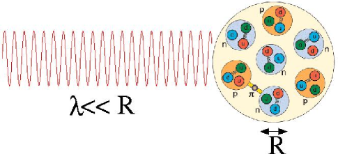
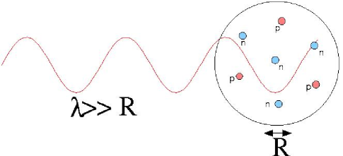
Figure 1: A short wavelength probe resolves quark and gluon degrees of freedom.

Figure 2: For long wavelength probes, low-energy degrees of freedom (protons and neutrons here) with simpler short-distance structure can be used.

2.1 Renormalization Group and NN Potential

We illustrate the general principle by considering nucleon-nucleon scattering in the center-of-mass frame (see Fig. 4). The Lippmann-Schwinger equation iterates a potential, which we can take as one of the $\chi^{2}/\mbox{dof}\approx 1$ potentials (as in Fig. 4). Intermediate states with relative momenta as high as $q=20\,\mbox{fm}^{-1}$ are needed for convergence of the sum in the second term. Yet the elastic scattering data and the reliable long-distance physics (pion exchange) only constrain the potential for $q\leq 3\,\mbox{fm}^{-1}$ SCHWENK03 .

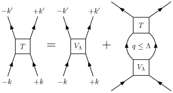
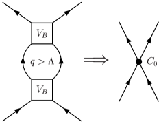
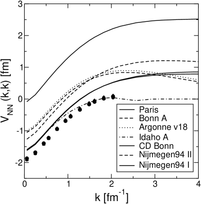
Figure 3: The equation for the $T$-matrix with cut-off potential $V_{\Lambda}$ and replacement of the effects of high $q$ intermediate states with a contact interaction.

Figure 4: The ${}^{1}S_{0}$ $V_{\Lambda}$ at $\Lambda=2.1\,\mbox{fm}^{-1}$ (symbols) for many $\chi^{2}/\mbox{dof}\approx 1$ potentials SCHWENK03 .

We can cut off the intermediate states at successively lower $\Lambda$; with each step we have to change the potential $V_{\Lambda}$ to maintain the same phase shifts. This determines the renormalization group (RG) equation for $V_{\Lambda}$ SCHWENK03 . We see in Fig. 4 that at $\Lambda=2.1\,\mbox{fm}^{-1}$, the potentials have all collapsed to the same low-momentum potential (“$V_{{\rm low\,}k}$”). We emphasize that this potential still reproduces all of the phase shifts described by the original potentials. The collapse actually occurs for $\Lambda$ between about 500 and 600 MeV (or 2.5–3 fm^-1), which implies model dependences at shorter distances. Note that the collapse does not mean that the short-distance physics is unimportant in the $S$ channels; rather, only the coarse features are relevant and a hard core is not needed. (For much more discussion of $V_{{\rm low\,}k}$, including plots of the potentials and phase shifts in all relevant channels, see SCHWENK03 .)

The shift of each bare potential to $V_{{\rm low\,}k}$ is largely constant at low momenta, which means it is well represented just by contact terms and a derivative expansion (i.e., a power series in momentum) SCHWENK03 . This observation illustrates explicitly that the short-distance physics can be absorbed into local terms; this is the essence of renormalization! Further, it motivates the use of a local Lagrangian approach. In an EFT, by varying the cutoff (or equivalent regularization parameter), we shift contributions between loops and low-energy constants (LEC’s), just like the shift between the high-lying intermediate state sum and the potential $V_{\Lambda}$. The long-range physics is treated explicitly (e.g., pion exchange) and short-distance interactions are replaced by LEC’s multiplying contact terms (including derivatives).

2.2 Effective Field Theory Ingredients

The low-energy data is insensitive to details of short-distance physics, so we can replace the latter with something simpler without distorting the low-energy physics. Effective field theory (EFT) is a local Lagrangian, model-independent approach to this program. Complete sets of operators at each order, determined by a well-defined power counting, lead to a systematic expansion, which means we can make error estimates. Underlying symmetries are incorporated and we generate currents for external probes consistent with the interactions. The natural hierarchy of scales is a source of expansion parameters.

The EFT program is realized as described in CROSSING :

1. Use the most general Lagrangian with low-energy degrees of freedom consistent with global and local symmetries of the underlying theory. For few-nucleon chiral EFT (our example here), this is a sum of Lagrangians for the zero, one, and two+ nucleon sectors of the strong interaction:

   $${\cal L}_{\rm eft}={\cal L}_{\pi\pi}+{\cal L}_{\pi N}+{\cal L}_{NN}\ .$$ (1)

   Chiral symmetry constrains the form of the long-distance pion physics, which allows a systematic organization of pion terms VANKOLCK99 .

2. Declare a regularization and renormalization scheme. For the few nucleon problem, the most successful approach has been to introduce a smooth cutoff in momentum. The success of the renormalization procedure is reflected in the sensitivity to the value of the cutoff. The change in observables with a reasonable variation of the cutoff gives an estimate of truncation errors for the EFT EPELBAUM .

3. Establish a well-defined power counting based on small expansion parameters. The source of expansion parameters in an EFT is usually a ratio of scales in the problem. For the strong interaction case, we have the momenta of nucleons and pions or the pion mass compared to a characteristic chiral symmetry breaking scale $\Lambda_{\chi}$, which is roughly 1 GeV (600 MeV is probably closer to the value in practice). The nuclear problem is complicated relative to $\pi\pi$ or $\pi N$ by an additional small scale, the deuteron binding energy, which precludes a perturbative expansion in diagrams. Weinberg proposed to power count in the potential and then solve the Schrödinger equation, which provides a nonperturbative summation that deals with the small scale. The NN potential is expanded as:

   $$V_{\rm NN}=\sum_{\nu=\nu_{\rm min}}^{\infty}c_{\nu}Q^{\nu}\ ,$$ (2)

   with $Q$ a generic momentum or the pion mass, and (see CROSSING for details)

   $$\nu=4-A+2(L-C)+\sum_{i}V_{i}(d_{i}+f_{i}/2-2)\ ,$$ (3)

   where the topology of the corresponding Feynman diagram determines $\nu$.

The organization of $V_{\rm NN}$ in powers of $Q$ is illustrated in this table (solid lines are nucleons, dotted lines are pions):

$Q^{\nu}$	1$\pi$	$2\pi$	$4N$
$Q^{0}$		—
$Q^{1}$
$Q^{2}$
$Q^{3}$

The table indicates what gets added at leading order (LO), next-to-leading order (NLO), and next-to-next-to-leading order (NNLO or N²LO). The low-energy constants at LO and NLO, which are the coefficients of the $4N$ contact terms (nine total), are determined by matching to the phase-shift data at energies up to 100 MeV; phases at higher energies are predictions. (There is also input from $\pi N$ scattering through ${\cal L}_{\pi N}$ at NNLO.)

Figure 5: Representative phase shifts at LO (dots), NLO (dashes), and NNLO (solid) as a function of lab energy (in GeV) EPELBAUM .

In Fig. 5, the systematic improvement from LO to NNLO is evident EPELBAUM . This type of systematic improvement is what we seek for the many-body problem. Recent calculations at N³LO by Entem and Machleidt ENTEM03 and by Epelbaum et al. EPELBAUM03 show continued improvement. The work by Epelbaum et al. is particularly noteworthy in providing error bands based on varying the cutoff. All of the phase shifts are consistently predicted within the estimated truncation error. Entem and Machleidt fine-tune their potential to achieve $\chi^{2}\approx 1$ for the phase-shift data up to 300 MeV lab energy. This puts the potential on the same footing as conventional potentials, but sacrifices the controlled systematics of the EFT.

An important feature of the chiral EFT is that it exhibits naturalness. That means that when the relevant dimensional scales for any given term are identified and factored out, the remaining dimensionless parameters are of order unity. If this were not the case, then a systematic hierarchy would be in jeopardy. The appropriate scheme for low-energy QCD, which Georgi and Manohar GEORGI84b called “naive dimensional analysis” (or NDA), assigns powers of $f_{\pi}=93\,\mbox{MeV}$ and $\Lambda_{\chi}$ to a generic term in the Lagrangian according to:

$${\cal L}_{\chi\,\rm eft}=c_{lmn}\left(\frac{N^{\dagger}(\cdots)N}{f_{\pi}^{2}\Lambda_{\chi}}\right)^{l}\left(\frac{\pi}{f_{\pi}}\right)^{m}\left(\frac{\partial^{\mu},m_{\pi}}{\Lambda_{\chi}}\right)^{n}f_{\pi}^{2}\Lambda_{\chi}^{2}\ ,$$ (4)

where $l$, $m$, and $n$ are integers.

The dimensionless constants resulting when the LO and NLO constants are scaled this way EPELBAUM are given in the table below for cutoffs ranging from 500 to 600 MeV. We see that $1/3\lesssim c_{lmn}\lesssim 3$ in all cases, with one exception, which implies they are natural (and the expansion is under control). The one exception is $f_{\pi}^{2}C_{T}$, which is unnaturally small. This is often a signal that there is a symmetry, and in this case a corresponding symmetry has indeed been identified: the Wigner $SU(4)$ spin-isospin symmetry EPELBAUM .

$f_{\pi}^{2}\,{C}_{S}$	$-1.079\ldots-0.953$	$f_{\pi}^{2}\,{C}_{T}$	$0.002\ldots 0.040$
$f_{\pi}^{2}\Lambda_{\chi}^{2}\,{C}_{1}$	$3.143\ldots 2.665$	$4\,f_{\pi}^{2}\Lambda_{\chi}^{2}\,{C}_{2}$	$2.029\ldots 2.251$
$f_{\pi}^{2}\Lambda_{\chi}^{2}\,{C}_{3}$	$0.403\ldots 0.281$	$4\,f_{\pi}^{2}\Lambda_{\chi}^{2}\,{C}_{4}$	$-0.364\ldots-0.428$
$2\,f_{\pi}^{2}\Lambda_{\chi}^{2}\,{C}_{5}$	$2.846\ldots 3.410$	$f_{\pi}^{2}\Lambda_{\chi}^{2}\,{C}_{6}$	$-0.728\ldots-0.668$
$4\,f_{\pi}^{2}\Lambda_{\chi}^{2}\,{C}_{7}$	$-1.929\ldots-1.681$

We can also explore the connection between the chiral EFT and conventional potentials by assuming that the boson-exchange potentials provide models of the short-distance physics that is unresolved in chiral EFT (except for the pion). Thus this physics should be encoded in coefficients of the contact terms. We can reveal the physics by expanding the boson propagators:

By comparing to (4) with $m\approx\Lambda_{\chi}$, we see that $g\sim\Lambda_{\chi}/f_{\pi}$, which explains the large couplings for phenomenological one-boson exchange!

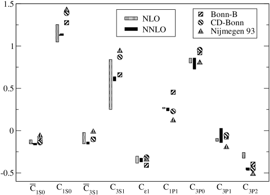
Figure 6: Comparison of EFT and one-boson-exchange coefficients EPELBAUM .

In Fig. 6, coefficients from the chiral EFT are compared to those obtained from such an expansion applied to several boson-exchange potentials EPELBAUM . The semi-quantitative agreement is remarkable and shows that there are strong similarities between the chiral potential and standard phenomenology. It is not yet clear, however, whether one can conclude that the potentials contain reasonable models of short-distance physics; the agreement may just reflect the fact that they all fit the same data.

In summary, the chiral EFT for two-nucleon physics (and few-body nuclei) is maturing rapidly. The systematic improvement and model independent nature is compelling. We seek the same characteristics for our description of heavier nuclei using covariant energy functionals.

3 Relativistic versus Nonrelativistic EFT for Nuclei

Why should one consider a relativistic effective field theory for nuclei? Let us first play devil’s advocate and argue the contrary case. The relevant degrees of freedom for low-energy QCD are pions and nucleons (at very low energy even pions are unresolved). Nuclei are clearly nonrelativistic, since the Fermi momentum $k_{\scriptscriptstyle\rm F}$ is small compared to the nucleon mass. The nonrelativistic NN EFT described above is close to the successful nonrelativistic potential and shows no (obvious) signs of problems.

In the past, a common argument against covariant treatments was that they intrinsically relied on “Z graphs,” which implied ${\rm\overline{N}N}$ contributions that were far off shell. The claim was that those should really come with form factors that would strongly suppress their contribution BRODSKY84 . This argument does not hold water in light of the effective theory principle we have highlighted: the high-energy, off-shell intermediate states may be incorrect, but that is fine, since the physics can be corrected by local counterterms. (Note: this only works if we include the appropriate local operators!) The modern EFT argument against Z graphs is different: since they are short-distance degrees of freedom, they should be integrated out. Indeed, it is often said that the heavy meson fields ($\sigma$, $\omega$, and so on) should be integrated out as well.

This argument is sometimes advanced as a matter of principle, but the underlying reason is the need for a well-defined power counting. The early experience with chiral perturbation theory using relativistic nucleons was that chiral power counting is spoiled by unwanted factors of the nucleon mass that come essentially from Z graphs GASSER88 . Integrating out heavy degrees of freedom moves these large scales to the denominators and then all is well JENKINS91 .

We’ll resolve the issue of power counting in the next subsections. But first a brief (in the legal sense) on the side of the (covariant) angels. Arguments in favor of covariant approaches to nuclear structure are collected in FURNSTAHL00 and FURNSTAHL00a ; this is merely a skeletal summary. For nuclear structure applications, the relevance of relativity is not the need for relativistic kinematics but that a covariant formulation maintains the distinction between scalars and vectors (more precisely, the zeroth component of Lorentz four-vectors). There is compelling evidence that representations with large scalar and vector fields in nuclei, of order a few hundred MeV, provide simpler and more efficient descriptions than nonrelativistic approaches that hide these scales. The dominant evidence is the spin-orbit splittings. Other evidence includes the density dependence of optical potentials, the observation of approximate pseudospin symmetry, correlated two-pion exchange strength, QCD sum rules, and more.

3.1 Historical Perspective: Relativistic Hartree Approximation

From the first applications of relativistic field theory to nuclear structure (“quantum hadrodynamics” or QHD), the Dirac sea had to be considered. Indeed, it was often hailed as being new physics missing from the nonrelativistic description. The simplest (and seemingly unavoidable) consequence of the Dirac sea was an energy shift from filled negative-energy states in the presence of a scalar field $\phi$ that shifts the effective nucleon mass to $M^{*}$ (i.e., a form of Casimir energy, see Fig. 7 for a schematic of shifted nucleon poles):

$$\delta H=-\sum_{{\bf k}\lambda}\bigl{[}({\bf k}^{2}+M^{*}{}^{2})^{1/2}-({\bf k}^{2}+M^{2})^{1/2}\bigr{]}\,;\qquad M^{*}\equiv M-g_{s}\phi$$ (5)

This sum is divergent. Two paths were taken to deal with the divergence. The “no-sea approximation” simply discards the negative-energy contributions (and therefore $\delta H$) with a casual argument about effective theories (we fix up this argument in EFT language below).

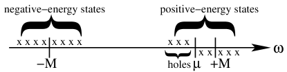
Figure 7: Pole structure for the single-particle propagator.

The other approach was to insist on renormalizability of the QHD theory. The usual prescription eliminated powers of $\phi$ up to $\phi^{4}$ in $\delta H$, leaving a finite shift in the energy in the “relativistic Hartree approximation” (RHA) of SEROT86

$$\Delta{\cal E}_{\rm RHA} = -{1\over 4\pi^{2}}\bigl{[}M^{*}{}^{4}\ln({M^{*}\over M})-\mbox{first four powers of $\phi$}\bigr{]}$$ (6)

$$= {5!\,\kappa_{5}\over 20\pi^{2}}M^{4}\Bigl{(}{\phi\over f_{\pi}}\Bigr{)}^{5}+{6!\,\kappa_{6}\over 120\pi^{2}}M^{4}\Bigl{(}{\phi\over f_{\pi}}\Bigr{)}^{6}+\cdots\ .$$ (7)

In accordance with Georgi-Manohar NDA, we have in the second line scaled $\phi$ with a factor of $f_{\pi}$ and introduced combinatoric factors and dimensionless couplings $\kappa_{5}$ and $\kappa_{6}$ of order unity (which absorb factors of $g_{s}f_{\pi}/M\approx 1$). The overall factor of $M^{4}$, however, is much larger than the corresponding factor of $f_{\pi}^{2}\Lambda_{\chi}^{2}$ in NDA. This is a signature that the power counting will not be correct.

Figure 8: Contributions to the energy per particle from terms in the RHA energy functional proportional to $\phi^{n}$ FURNSTAHL97b . Two values of $M^{*}/M$ are considered (diamonds and squares). The X’s and error bars reflect natural NDA estimates.

In practice, the $\phi^{5}$ and higher terms are large and drive the self-consistent effective mass $M^{*}$ too close to $M$, which results in too small spin-orbit splittings (the raison d’etre of the relativistic approach!). Furthermore, the loop expansion is a phenomenological disaster (two-loop corrections qualitatively change the physics and there is no sign of convergence FURNSTAHL89 ). The $M^{4}$ factor in (7) also badly violates $N_{c}$ counting that we would expect in a low-energy theory of QCD. ($N_{c}$ is the number of colors.) With $\Lambda_{\chi}$ associated with a meson mass, $M^{4}\propto(N_{c})^{4}$ while $\Lambda_{\chi}^{2}f_{\pi}^{2}\propto(1)^{2}(N_{c}^{1/2})^{2}\propto(N_{c})^{1}$ FURNSTAHL97b .

In general, the RHA energy functional exhibits unnaturally large contributions to $\phi^{n}$ terms, as seen in Fig. 8. A natural effective theory would have decreasing contributions, so that $\phi^{5}$ and higher terms would have only minor effects (easily absorbed elsewhere). With a value of $M^{*}/M\approx 0.6$, which is required for realistic spin-orbit splittings, the energy/particle from the $\phi^{5}$ term is two orders of magnitude too large. The system adjusts $M^{*}$ upward to reduce this contribution, but the consequence is small spin-orbit splittings.

3.2 Power Counting Lost / Power Counting Regained

Gasser, Sainio, and Svarc first adapted chiral perturbation theory (ChPT) to pion-nucleon physics using relativistic nucleons GASSER88 . In contrast to the pion-only sector, however, the loop and momentum expansions did not agree and systematic power counting was lost. The heavy-baryon formulation was introduced to restore power counting through an expansion in $1/M$, which means a nonrelativistic formulation JENKINS91 .

In 1996, Hua-Bin Tang wrote a seminal paper TANG96 in which he said “…EFT’s permit useful low-energy expansions only if we absorb all of the hard-momentum effects into the parameters of the Lagrangian.” The key observation he made was that: “When we include the nucleons relativistically, the anti-nucleon contributions are also hard-momentum effects.” Once the “hard” part of a diagram is absorbed into parameters, the remaining “soft” part satisfies chiral power counting.

There are several prescriptions on the market for carrying out this program. Tang’s original prescription (developed with Ellis) involved the expansion and resummation of propagators TANG96 ; ELLIS98 . This basic idea was systematized for $\pi N$ by Becher and Leutwyler BECHER99 under the name “infrared regularization.” More recently, Fuchs et al. described an alternative prescription using additional finite subtractions (beyond minimal subtraction) in dimensional regularization FUCHS03 . Goity et al. GOITY01 and Lehmann and Prézeau Lehmann:2001xm extended infrared regularization to multiple heavy particles. The result for particle-particle loops reduces to the usual nonrelativistic result for small momenta while particle-hole loops in free space vanish identically.

3.3 Effective Action and the No-Sea Approximation

At the one-loop level, we will be able to apply the necessary subtractions without specifying the regularization and renormalization prescription in detail. It is convenient to use an effective action formalism to carry out the EFT at finite density. The effective action is obtained by functional Legendre transformation of a path integral generating functional with respect to source terms. This is analogous to Legendre transformations in thermodynamics. We assume some familiarity with effective actions; see ILIOPOULOS ; NEGELE88 ; PESKIN95 ; WEINBERG96 to learn more.

QHD models with heavy-meson fields correspond to effective actions with auxiliary fields, introduced to reduce the fermion integration to just a gaussian integral. We denote the effective action $\Gamma[\phi,V^{\mu}]$, with classical fields $\phi$ and $V^{\mu}$ (suppressing all other fields) FURNSTAHL89 . An alternative is to work with a point coupling model, in which case the effective action will be a functional of the scalar nucleon density and the vector current.

There will always be a gaussian fermion integral, which yields a determinant that appears in the effective action as the trace over space-time and internal variables of the logarithm of a differential operator:

$${\rm Tr\ }\!\ln(i\!\!\not\!\partial+\mu\gamma^{0}-M^{*}-g_{{\rm v}}\!\!\not\!V)\equiv{\rm Tr\ }\!\ln G^{-1}\ .$$ (8)

In the point-coupling case, optical potentials that are functions of the density and current appear directly rather than through meson fields, but the form is the same as (8). This ${\rm Tr\ }\!\ln$ depends on $\mu$, the nucleon chemical potential.

The derivative expansion of the ${\rm Tr\ }\!\ln$ at $\mu=0$ takes the form PERRY86 :

$$-i\,{\rm Tr\ }\!\ln(i\!\!\not\!\partial-M^{*}-g_{{\rm v}}\!\!\not\!V) = \int\!d^{4}x\ \bigl{[}U_{\rm eff}(\phi)+\frac{1}{2}Z_{1s}(\phi)\partial_{\mu}\phi\partial^{\mu}\phi$$ (9)

$$\quad\hbox{}+\frac{1}{2}Z_{2s}(\phi)(\square\phi)^{2}+\cdots\bigr{]}\ ,$$

which shows that this is a purely local potential in the meson fields. This means it can be entirely absorbed into local terms in the Lagrangian. That is, by adjusting the constants appropriately, this contribution to the energy will not appear. We specify a consistent subtraction at a specific $\mu$, which means removing a set of local terms (that are implicitly absorbed by parameter redefinition). The obvious choice is $\mu=0$.

We can accomplish this in practice at $\mu\neq 0$ simply by performing a subtraction of the ${\rm Tr\ }\!\ln$ evaluated at $\mu=0$. Note that this is not a vacuum subtraction, because it depends on the finite-density background fields $\phi(x)$ and $V^{\mu}(x)$. It is simply a choice for shifting “hard” Dirac sea physics into the coefficients. We emphasize that the same coefficients in the derivative expansion are subtracted for any background fields. For the ground state, this will simply remove all explicit evidence of the negative-energy states. But there are fixed consequences for treating linear response (RPA) that still involve negative-energy states FURNSTAHL87 ; SHEPARD89 ; DAWSON90 ; Furnstahl:2002fz .

For the ground state, field equations for the meson potentials are obtained by extremizing $\Gamma[\phi,V^{\mu}]$. These equations determine static potentials $\phi_{0}({\bf x})$ and $V_{0}({\bf x})$ for the ground state; the corresponding Green’s function is the Hartree propagator, denoted $G_{H}$. Then $\Gamma[\phi_{0}({\bf x}),V_{0}({\bf x})]$ is proportional to the zero-temperature thermodynamic potential $\Omega=E-\mu N$. Both $+i\,{\rm Tr\ }\!\ln G_{H}^{-1}(\mu)$ and $+i\,{\rm Tr\ }\!\ln G_{H}^{-1}(0)$ are diagonal in the same single-particle basis $\psi_{\alpha}({\bf x})e^{i\omega x_{0}}$, where the $\psi_{\alpha}({\bf x})$’s are solutions with eigenvalues $\epsilon_{\alpha}$ to the Dirac equation in the static potentials. Thus the subtraction is simple ($T$ is a constant time that cancels out):

(10)

where we have omitted the parts of $\Gamma$ (and $\Omega$) depending only on meson potentials, and the vacuum subtraction for the baryon number FURNSTAHL95 ; Furnstahl:2002fz . Thus the contribution to the energy is simply a sum over occupied, positive-energy, single-particle eigenvalues. This is the “no-sea” prescription!

Similarly, we can calculate the scalar density (the expectation value of $\overline{\psi}\psi$) from the effective action, which yields

$$\rho_{s}({\bf x})\propto\delta\Gamma/\delta(g_{s}\phi({\bf x}))\Longrightarrow{\rm Tr\ }G_{H}(\mu)-{\rm Tr\ }G_{H}(0)\ .$$ (11)

The subtraction removes the contribution from the sum over negative-energy states. This is indicated diagrammatically as :

where “$h$” denotes holes and “$-$” denotes negative-energy states. Thus, we recover the “no-sea approximation” for the ground state. What is the corresponding result for RPA excitations?

Consider $\Gamma[\phi,V^{\mu}]$ evaluated with time-dependent fluctuations about the static ground-state potentials:

$$\phi(x)=\phi_{0}({\bf x})+{\widetilde{\phi}(x)}\ ,\qquad V^{\mu}(x)=V_{0}({\bf x})\,\delta_{\mu 0}+{\widetilde{V}^{\mu}(x)}\ .$$ (12)

We can access the linear response directly from the effective action, because $\Gamma$ is the generator of one-particle-irreducible Green’s functions PESKIN95 . The linear response is dictated by the second-order terms in powers of $\widetilde{\phi},\widetilde{V}^{\mu}$. So we expand

$$\Gamma=-i\,{\rm Tr\ }\!\ln G^{-1}(\mu)+i\,{\rm Tr\ }\!\ln G^{-1}(0)+\ldots$$ (13)

in $\widetilde{\phi},\widetilde{V}^{\mu}$ (this generates the “polarization insertion”):

$$\ln(G_{H}^{-1}+g_{s}\widetilde{\phi})=\ln(G_{H}^{-1})\bigl{[}\ldots-\frac{1}{2}G_{H}\,(g_{s}\widetilde{\phi})\,G_{H}\,(g_{s}\widetilde{\phi})+\ldots\bigr{]}\ .$$ (14)

The two $G_{H}$’s mean that we generate rings with Hartree propagators:

$$-i\,{\rm Tr\ }\!\ln G^{-1}(\mu)\Longrightarrow\raisebox{-0.86108pt}{\parbox{72.26999pt}{\includegraphics*[width=72.26999pt,angle={0}]{fig_rpa3bw}}}\quad-i\,{\rm Tr\ }\!\ln G^{-1}(0)\Longrightarrow\raisebox{-0.86108pt}{\parbox{32.52127pt}{\includegraphics*[width=32.52127pt,angle={0}]{fig_rpa4bw}}}$$ (15)

but different spectral content. Combining these contributions as in (13):

We see that the consistent prescription for the RPA is to include particle-hole pairs ($ph$) and pairs formed from holes and negative-energy states ($h-$).

The lesson from effective field theory is that we must absorb hard-momentum Dirac-sea physics into the parameters of the energy functional. This explains the successful relativistic mean-field and RPA “no-sea” phenomenology. The QCD vacuum effects are automatically encoded in the fit parameters; there is no need to refit at different densities. In principle, to absorb all of the short-distance physics we need all possible counterterms. In practice, we rely on naturalness to make truncations (which justifies the success of conventional models with limited terms).

The effective action formalism is a natural framework for systematically extending the one-loop treatment. By embedding the “mean-field” models within the density functional theory (DFT) framework, we realize that correlations are approximately included with the present-day mean-field functionals, which can be generalized to systematically improve them according to EFT power counting. Note that the effective action formulation leads naturally to time-dependent DFT as well. To carry out this program, a generalized infrared regularization scheme (or equivalent, possibly with a cutoff) is needed.

4 Toward More Systematic Energy Functionals

The energy functionals of relativistic mean-field models need improvement in a number of areas. As stressed in our first discussion of EFT’s, long-range physics must be included explicitly. However, chiral physics as manifested in long-range pion interactions is not included explicitly in mean-field models and the treatment of long-range correlations is unlikely to be adequate. Pairing is still more an art than a science. Isovector physics in general has problems, as asymmetric ($N\neq Z$) nuclear matter is poorly constrained. Here we focus on the last of these.

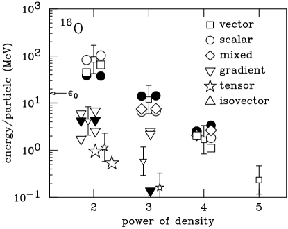
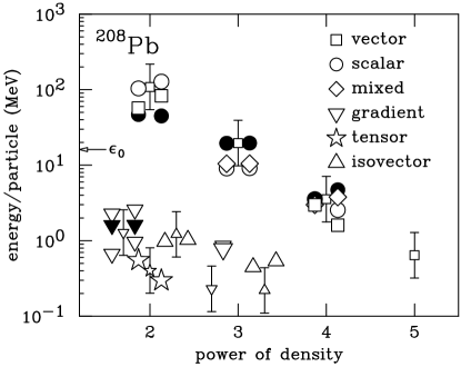
Figure 9: Estimates in finite nuclei using averages of densities and results from two models (at left and right of error bars) FURNSTAHL00a .

EFT-inspired power counting (in the form of NDA FRIAR96 ) can be applied to mean-field energy functionals to quantify the isovector constraints. Estimates of individual contributions in a given functional to the energy per particle of a finite nucleus can be made using NDA rules to associate powers of $f_{\pi}$ and $\Lambda_{\chi}$ with scalar ($\rho_{s}$), baryon ($\rho_{{\scriptscriptstyle\rm B}}$), isovector ($\rho_{3}$), and tensor (${{s}}$) densities and gradients:

$$\widetilde{\rho}_{{\scriptstyle\rm s}},\widetilde{\rho}_{{\scriptscriptstyle\rm B}}\rightarrow{\displaystyle\langle\rho_{{\scriptscriptstyle\rm B}}\rangle\over\displaystyle\ts f_{\pi}^{2}\Lambda}\quad\widetilde{{{\hbox{\boldmath$\displaystyle\nabla$}}}}\rho_{{\scriptscriptstyle\rm B}}\rightarrow{\displaystyle\langle{{{\hbox{\boldmath$\displaystyle\nabla$}}}}\rho_{{\scriptscriptstyle\rm B}}\rangle\over\displaystyle\ts f_{\pi}^{2}\Lambda^{2}}\quad\widetilde{{s}}\rightarrow{\displaystyle\langle\widetilde{{s}}\rangle\over\displaystyle\ts f_{\pi}^{2}\Lambda}\quad\widetilde{\rho}_{3}\rightarrow{\displaystyle Z-N\over\displaystyle\ts 2A}{\displaystyle\langle\rho_{{\scriptscriptstyle\rm B}}\rangle\over\displaystyle\ts f_{\pi}^{2}\Lambda}$$ (16)

and then using local density approximations to estimate the densities. Typical results are shown in Fig. 9. The hierarchy of isoscalar contributions is clear and shows that three orders of parameters can be constrained (contributions below about 1 MeV are not constrained). In contrast, the isovector parameters are weakly constrained by the energy; essentially only one parameter is determined. Naturalness implies that the $({{{\hbox{\boldmath$\displaystyle\nabla$}}}}\rho_{3})^{2}$ contribution to observables such as the skin thickness $r_{n}-r_{p}$ is small (see FURNSTAHL02b ), so we can focus on terms in the functional that contribute for uniform systems. This leads us to examine the symmetry energy in uniform matter.

4.1 Power Counting and the Symmetry Energy

The relationship between the neutron skin in ²⁰⁸Pb and the symmetry energy in uniform matter has been studied in detail OYAMATSU98 ; BROWN00 ; TYPEL01 ; FURNSTAHL02b ; DANIELEWICZ03 . We can frame the discussion in terms of the energy per particle $E(\rho,\alpha)$ in asymmetric matter, which can be expanded as:

$$E(\rho,{\alpha})=E(\rho,{0})+S_{2}(\rho){\alpha^{2}}+S_{4}(\rho){\alpha^{4}}+\cdots\qquad{\alpha\equiv{N-Z\over A}}$$ (17)

where $\rho$ is the baryon density and $\alpha$ is an asymmetry parameter. The $\alpha=0$ term has the usual expansion around the saturation density $\rho_{0}$:

$$E(\rho,0)=-{a_{\rm v}}+{K_{0}\over 18\rho_{0}^{2}}(\rho-\rho_{0})^{2}+\cdots$$ (18)

while the quadratic symmetry energy $S_{2}(\rho)$ is expanded as:

$${S_{2}(\rho)}={a_{4}}+{{p_{0}}\over\rho_{0}^{2}}(\rho-\rho_{0})+{\Delta K_{0}\over 18\rho_{0}^{2}}(\rho-\rho_{0})^{2}+\cdots$$ (19)

Two key parameters are the symmetry energy at saturation, $a_{4}$, and the linear density dependence, $p_{0}$. (Note: $S_{4}(\rho)$ is unimportant numerically.)

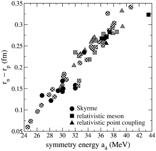
Figure 10: Skin thickness in ²⁰⁸Pb versus the equilibrium symmetry energy FURNSTAHL02b .

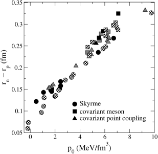
Figure 11: Skin thickness in ²⁰⁸Pb as a function of the density dependence of the symmetry energy FURNSTAHL02b .

A study of a wide range of mean-field models, both nonrelativistic Skyrme and relativistic mean-field (meson-based and point-coupling), show strong correlations between the skin thickness in ²⁰⁸Pb and the symmetry energy parameters. In Figs. 10 and 11, this correlation is shown explicitly. While there is a large spread in the values of $S_{2}(\rho_{0})=a_{4}$, if we plot the spread (i.e., the standard deviation) as a function of $\rho$, we see that the spread is smallest at a density corresponding to the average density in heavy nuclei (see Fig. 12). This result is consistent with our conclusion from power counting that only one parameter is determined: it is the symmetry energy at some lower density.

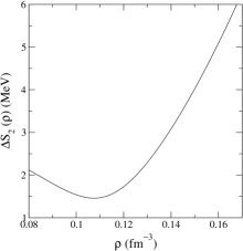
Figure 12: The spread (standard deviation) of $S_{2}(\rho)$ [see (17)] for many mean-field models fit to nuclear bulk properties FURNSTAHL02b .

Since $p_{0}$ is a pressure that pushes neutrons out against the surface tension in ²⁰⁸Pb, it is instrumental in determining the skin thickness Horowitz:2001ya . How well do we know its value? A comparison of symmetry energies predicted by realistic non-relativistic potentials was made in MACHLEIDT with the result in Fig. 13. Reading off the slopes implies that $p_{0}\approx 2.1\,\mbox{MeV/fm}^{-3}$ with only a 10% spread. From relativistic RBHF calculations, $p_{0}\approx 3.3\,\mbox{MeV/fm}^{-3}$. In either case, there is a strong discrepancy with conventional meson mean-field models, which have $p_{0}\geq 4$.

Figure 13: Comparison of the symmetry energy for realistic potentials MACHLEIDT .

This conclusion is supported by Danielewicz DANIELEWICZ03 , who has analyzed the relationship in terms of surface vs. volume symmetry energies. Using mass formula constraints in conjunction with skin thickness analysis, he concludes that $0.56\leq S_{2}(\rho_{0}/2)/a_{4}\leq 0.81$, which allows the models between the vertical lines in Fig. 14. Once again, conventional relativistic models are excluded.

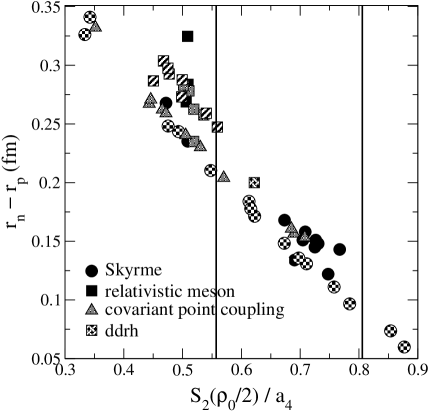
Figure 14: Skin thickness in ²⁰⁸Pb versus the normalized density dependence of the symmetry energy.

There are several ways out. Point coupling NIKOLAUS97 ; RUSNAK97 , DDRH Fuchs:1995as ; Niksic:2002yp , and new relativistic mean-field models (with mesons) Horowitz:2001ya get lower values of $p_{0}$ by adding isovector parameters (implicitly, in the case of DDRH). However, they achieve lower $p_{0}$ from an unnatural cancellation between different orders according to the present power counting FURNSTAHL02b . This doesn’t mean it is wrong, but it means we haven’t captured the physics of the symmetry energy. For example, it might be pion physics with a different functional form. These results imply that we should revisit the symmetry energy in covariant models within a chiral EFT.

4.2 Guidance from DFT for Solid-State or Molecular Systems

The density functional theory (DFT) perspective helps to explain successful “mean-field” phenomenology, but DFT existence theorems are not constructive. NDA power counting gives guidance on truncation but not on the analytic form of functionals. One approach toward more accurate energy functionals would be to emulate the quantum chemists.

The Hohenberg-Kohn free-energy for an inhomogeneous electron gas in an external potential takes the form ($n({\mathbf{x}})$ is the charge density here)

$$F_{{\rm HK}}[n({\mathbf{x}})]=F_{{\rm ni}}[n({\mathbf{x}})]+\frac{e^{2}}{2}\!\int\!d^{3}x\,d^{3}x^{\prime}\frac{n({\mathbf{x}})n({\mathbf{x}^{\prime}})}{|{\bf x}-{\bf x^{\prime}}|}+E_{{\rm xc}}[n({\mathbf{x}})]\ ,$$ (20)

where the direct Coulomb piece is explicit and the Kohn-Sham non-interacting functional is evaluated using

$$F_{{\rm ni}}[n({\mathbf{x}})]=\sum_{i=1}^{A}\langle\psi_{i}|\hat{t}_{i}|\psi_{i}\rangle=\sum_{i=1}^{N}\epsilon_{i}-\int\!d^{3}x\,n({\mathbf{x}})v_{\rm eff}({\mathbf{x}})\ .$$ (21)

The $\psi_{i}$’s are solutions to

$$\Bigl{(}-\frac{\hbar^{2}}{2m}\nabla^{2}+v_{\rm eff}({\mathbf{x}})\Bigr{)}\psi_{i}({\mathbf{x}})=\epsilon_{i}\psi_{i}({\mathbf{x}})$$ (22)

with the property that the exact density of the full system is given by

$$n({\mathbf{x}})=\sum_{i=1}^{N}|\psi_{i}({\mathbf{x}})|^{2}\ ,$$ (23)

which is the density of a noninteracting system with effective potential

$$v_{\rm eff}=v-e\phi+v_{\rm xc}\ ,\quad\mbox{where}\quad v_{\rm xc}({\mathbf{x}})\equiv\delta E_{\rm xc}/\delta n({\mathbf{x}})\ .$$ (24)

$v$ is the external potential, and $\phi$ is the Hartree potential.

Solving for the orbitals and energies is the easy part. The hard part is finding a reliable approximation to the exchange-correlation functional $E_{{\rm xc}}$. The approach used by quantum chemists uses the local density approximation

$$E_{{\rm xc}}[n({\mathbf{x}})]\approx\int\!d^{3}x\,{\cal E}_{{\rm xc}}(n({\mathbf{x}}))\ ,$$ (25)

where the energy density ${\cal E}_{{\rm xc}}$ is fit to a Monte Carlo calculation of the homogeneous electron gas (see Fig. 15). In practice, one uses parametric formulas, such as

$${\cal E}_{\rm xc}(n)/n=-0.458/r_{s}-0.0666G(r_{s}/11.4)$$ (26)

with

$$G(x)=\frac{1}{2}\left\{(1+x)^{3}\log(1+x^{-1})-x^{2}+\frac{1}{2}x-\frac{1}{3}\right\}$$ (27)

(the ones in common use are more sophisticated). The calculational procedure, which includes correlations through $E_{{\rm xc}}$, has the form of a “naive” mean-field approach with the additional potential

$$v_{\rm xc}=\left.\frac{d[{\cal E}_{\rm xc}(n)]}{dn}\right|_{n=n({\mathbf{x}})}\ .$$ (28)

An example of a successful atomic LDA calculation is shown in Fig. 16. Significant improvements to the LDA are made using (generalized) gradient expansions PERDEW96 ; PERDEW99 . The DDRH approach to relativistic energy functionals for nuclei, in which the density dependence of a nuclear matter calculation is incorporated through density-dependent couplings Fuchs:1995as ; Niksic:2002yp , is in the spirit of these LDA plus gradient expansion approaches.

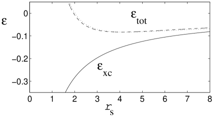
Figure 15: The exchange-correlation functional for a uniform system ($r_{s}\propto 1/k_{\scriptscriptstyle\rm F}$) ARGAMAN00 .

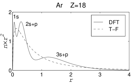
Figure 16: The charge density for argon atom calculated using DFT (in the LDA) and the Thomas-Fermi approximation ARGAMAN00 .

While there are many successes to be found, it is also clear that the situation is not entirely satisfactory. From A Chemist’s Guide to DFT KOCH2000 :

“To many, the success of DFT appeared somewhat miraculous, and maybe even unjust and unjustified. Unjust in view of the easy achievement of accuracy that was so hard to come by in the wave function based methods. And unjustified it appeared to those who doubted the soundness of the theoretical foundations.”

From Argaman and Makov’s article ARGAMAN00 (highly recommended!):

“It is important to stress that all practical applications of DFT rest on essentially uncontrolled approximations, such as the LDA …”

and from the authors of the state-of-the-art gradient approximations PERDEW96 :

“Some say that ‘there is no systematic way to construct density functional approximations.’ But there are more or less systematic ways, and the approach taken …here is one of the former.”

Thus we are motivated to consider a more systematic approach: EFT!

4.3 DFT in Effective Field Theory Form

It is particularly natural to consider DFT in thermodynamic terms, in analogy to finding via Legendre transformation the energy as a function of particle number from the thermodynamic potential as a function of the chemical potential ARGAMAN00 . This analogy implies the effective action formalism will be well suited. The EFT will provide power counting for diagrams and gradient expansions, thereby systematically approximating a model-independent functional. The EFT tells us how to renormalizes divergence consistently and gives insight into analytic structure of the functional.

As a laboratory for exploring DFT/EFT, we can consider a dilute “natural” Fermi gas in a confining potential, which is realized experimentally by cold atomic Fermi gases in optical traps. Natural in this context means that the scattering length is comparable to the range of the potential (rather than being fine tuned to a large value). The EFT Lagrangian takes the form

$${\cal L}_{\rm eft}=\psi^{\dagger}\bigl{[}i\frac{\partial}{\partial t}+\frac{\nabla^{\,2}}{2M}\bigr{]}\psi-\frac{{C_{0}}}{2}(\psi^{\dagger}\psi)^{2}-\frac{{D_{0}}}{6}(\psi^{\dagger}\psi)^{3}+\ldots$$ (29)

where the parameters can be determined from free-space scattering (or by finite density fits); dimensional regularization with minimal subtraction is particularly advantageous. The EFT for the uniform system (no external potential) predicts the energy (and other observables) simply and efficiently through a diagrammatic expansion, with a power counting that tells us what diagram to calculate at each order in the expansion. [See HAMMER00 for details.] The first terms in the diagrammatic expansion are (the solid dot is $C_{0}=4\pi a_{s}/{M}$, with $a_{s}$ the scattering length):

which yields the expansion for the energy density (with degeneracy $g$):

$${\cal E}=n\frac{{k_{\scriptscriptstyle\rm F}^{2}}}{2M}\biggl{[}\frac{3}{5}+(g-1)\biggl{\{}\frac{2}{3\pi}{(k_{\scriptscriptstyle\rm F}a_{s})}+\frac{4}{35\pi^{2}}(11-2\ln 2){(k_{\scriptscriptstyle\rm F}a_{s})^{2}}\biggr{\}}+\cdots\biggr{]}$$ (30)

in powers of $k_{\scriptscriptstyle\rm F}a_{s}$. (Note this is not a power series; see HAMMER00 .) The point here is that we have a systematic expansion: LO, NLO, NNLO, and so on, just as in the chiral NN case. To put the gas in a harmonic or gaussian trap with external potential $v({\bf x})$, we simply add a $v({\bf x})\rho({\bf x})$ term to the Lagrangian.

The effective action formalism starts with a path integral for the generating functional with an additional source $J$ coupled to the density:

$$Z[J]=e^{iW[J]}=\int\!{\cal D}\psi^{\dagger}{\cal D}\psi\ e^{i\int\!d^{4}x\,[{\cal L}-{J(x)\psi^{\dagger}(x)\psi(x)}]}\ .$$ (31)

(Different external sources can be used.) The density is found by a functional derivative with respect to $J$:

$$\rho(x)\equiv\langle\psi^{\dagger}(x)\psi(x)\rangle_{J}=\frac{\delta W[J]}{\delta J(x)}\ .$$ (32)

The crucial step is the inversion of (32); that is, to find $J[\rho]$. Given that, the effective action $\Gamma[\rho]$ follows from a functional Legendre transformation:

$$\Gamma[\rho]=W[J]-\int\!d^{4}x\,J(x)\rho(x)\ .$$ (33)

The functional $\Gamma[\rho]$ is proportional (with a trivial time factor) to the ground-state energy functional $E[\rho]$ that we seek. The density $\rho(x)$ is determined by stationarity:

$$\frac{\delta\Gamma[\rho]}{\delta\rho(x)}=-J(x)\Longrightarrow 0\mbox{\ \ in the ground state.}$$ (34)

That’s density functional theory in a nutshell!

Two approaches to invert the Legendre transformation have been proposed. They correspond to generating point coupling or meson-based models. We’ll outline the first approach, which is the inversion method of Fukuda et al. Fukuda:im ; VALIEV97 . It is a generalization of the Kohn-Luttinger inversion procedure KOHN60 . The idea is to use an order-by-order matching in a counting parameter $\lambda$, which we identify with an EFT expansion parameter (e.g., $1/\Lambda_{\chi}$). We expand each of the ingredients of (34):

$$J[\rho,\lambda] \!=\! J_{0}[\rho]+\lambda J_{1}[\rho]+\lambda^{2}J_{2}[\rho]+\cdots$$ (35)

$$W[J,\lambda] \!=\! W_{0}[J]+\lambda W_{1}[J]+\lambda^{2}W_{2}[J]+\cdots$$ (36)

$$\Gamma[\rho,\lambda] \!=\! \Gamma_{0}[\rho]+\lambda\Gamma_{1}[\rho]+\lambda^{2}\Gamma_{2}[\rho]+\cdots$$ (37)

and equate each order in $\lambda$. Zeroth order corresponds to a noninteracting system with potential $J_{0}(x)$:

$$\Gamma_{0}[\rho]=W_{0}[J_{0}]-\int\!d^{4}x\,J_{0}(x)\rho(x)\quad\Longrightarrow\quad\rho(x)=\frac{\delta W_{0}[J_{0}]}{\delta J_{0}(x)}\ .$$ (38)

This is the Kohn-Sham system with the exact density! That is, $J_{0}$ is the potential that reproduces the exact interacting density in a non-interacting system. We diagonalize $W_{0}[J_{0}]$ by introducing Kohn-Sham orbitals, which yields a sum of eigenvalues. Finally, we find $J_{0}$ for the ground state by completing a self-consistency loop:

$$J_{0}\rightarrow W_{1}\rightarrow\Gamma_{1}\rightarrow J_{1}\rightarrow W_{2}\rightarrow\Gamma_{2}\rightarrow\cdots\Longrightarrow J_{0}(x)=\sum_{i}\frac{\delta\Gamma_{i}[\rho]}{\delta\rho(x)}\ .$$ (39)

We can contrast the conventional expansion of the propagator:

$\Longrightarrow\$

which involves a non-local, state dependent $\Sigma^{\ast}({\bf x},{\bf x}^{\prime};\omega)$, with the local $J_{0}({\bf x})$:

To carry out this construction there are new Feynman rules that involve this “inverse density-density correlator,” which is indicated by a double line:

Complete details are available in PUGLIA03 .

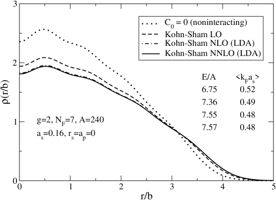
Figure 17: Density profiles for a dilute Fermi gas in a harmonic trap for successive approximations.

If we restrict the application to closed shells for simplicity, we just specify the spin degeneracy $g$ and the Fermi harmonic oscillator shell (the last occupied shell) $N_{F}$, which then determines the number $A$ of atoms. The iteration procedure for the dilute Fermi gas in a harmonic trap is as follows:

1. guess an initial density profile $\rho(r)$ (e.g., Thomas-Fermi),

2. evaluate the local single-particle potential $v_{\rm eff}(r)\equiv v(r)-J_{0}(r)$,

3. solve for the lowest $A$ states (including degeneracies) $\{\psi_{\alpha},\epsilon_{\alpha}\}$:

   $$\bigl{[}-\frac{{\nabla}^{2}}{2M}+v_{\rm eff}(r)\bigr{]}\,\psi_{\alpha}({\bf x})=\epsilon_{\alpha}\psi_{\alpha}({\bf x})\ ,$$ (40)

4. compute a new density $\rho(r)=\sum_{\alpha=1}^{A}|\psi_{\alpha}({\bf x})|^{2}$; other observables are functionals of $\{\psi_{\alpha},\epsilon_{\alpha}\}$,

5. repeat 2.–4. until changes are small (“self-consistent”).

This procedure is simple to implement as a computer program and will be familiar to anyone who has performed a relativistic mean-field calculation for finite nuclei.

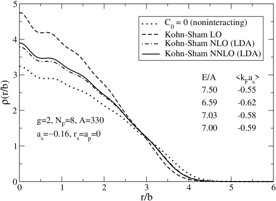
Figure 18: Density profiles for a dilute Fermi gas in a harmonic trap for successive approximations.

Some representative results are given in Figs. 17 and 18. Note the convergence of the densities and energies as we increase the order of the calculation. In Fig. 19, we show the contribution to the energy per particle at LO, NLO, and NNLO for three different systems. We estimate the expected contribution by NDA from the Hartree terms in the functional (which appear with simple powers of the density) and then scale correction terms by the expansion parameter $\langle k_{\scriptscriptstyle\rm F}\rangle a_{s}$. The power counting still works! This is an excellent laboratory to explore such issues. For example, the rightmost circle shows a large discrepancy between predicted and actual values. A closer examination reveals an “accidental” cancellation (that goes away for different parameter choices!).

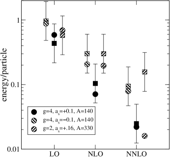
Figure 19: Energy estimates (squares) and actual values (circles) for a dilute system.

Although we did not discuss covariant DFT here, Schmid et al. have already laid the foundation SCHMID95 . The generalization of DFT to other sources and time dependence is straightforward (cf. spin-density functionals for Coulomb systems). For the covariant case, one treats $\overline{\psi}_{i}\psi_{j}$ as a matrix and introduces a source $j_{ij}$ coupled to it, which yields a functional of the scalar density and vector current, as described in Sect. 3.3.

5 Building the Next Generation Theories

The successes of chiral EFT for nucleon-nucleon scattering and the few-body problem have raised the bar for models of nuclear structure. For the next generation, we must justify what we do and not just mumble “effective theory” to account for phenomenological successes. This requires that we develop and test systematic power counting schemes and reexamine and sharpen arguments for a covariant approach. To meet the challenge, the next generation of covariant models must move away from model dependence. This implies turning away from the “minimal model” philosophy and including all terms allowed by symmetries (up to redundancies). It means requiring error estimates and a controlled expansion in density, asymmetry, and momentum transfer. And it means that the results should exhibit regulator (e.g., cutoff) independence up to expected truncation errors.

There has been significant progress made toward building the next generation of covariant approaches to nuclear structure (e.g., see B.D. Serot’s lecture). But there is a long list of loose ends to address. Some of the physics goals and open issues are

• a reliable description of nuclei far from stability;

• controlled equation of state and transport properties of neutron stars;

• unified description of collective excitations;

• currents, both elastic and transition currents to excited states;

• improved treatment of isovector physics;

• consistent incorporation of chiral physics;

• consistent treatment of pairing in covariant density functionals;

• establishing more direct connections to QCD (e.g., quark mass dependence of equilibrium properties).

The framework we have proposed to address these goals and issues is a merger of effective field theory and density functional theory. The idea is to embed the successful relativistic mean-field phenomenology into this framework, as traditional NN interactions are taken over by chiral EFT. The basic structure and successes are preserved, but model dependence is removed.

There are many challenges. For the covariant many-body EFT, one needs a consistent application of infrared regularization (or equivalent) applied at finite density. This is likely to mean the use of cutoff regularization. A possible laboratory for these issues is a dilute Fermi gas with $\Lambda\sim M_{N}$, where in a finite system the spin-orbit force can be directly explored. In addition, chiral EFT expansions must be translated to covariant form. For the covariant DFT, one needs systematic derivative expansions (analogous to past density matrix expansions), the incorporation of long-range forces and pairing, and a consistent extension to time-dependent DFT. Most importantly, we need a more complete power counting scheme for energy functionals.

There is growing hope for an ultimate path to ab initio calculations of nuclei, starting from quantum chromodynamics (QCD). Nonperturbative lattice QCD could calculate low-energy constants needed for the chiral EFT of NN and few-body systems. This EFT in turn determines the analytic structure and low-energy constants of a (covariant) many-body EFT, which takes the form of a DFT energy functional, applicable across the periodic table. There are many gaps, but this dream has become significantly more plausible at all levels in just the last few years.

References

- (1) P. Ring: Prog. Part. Nucl. Phys. 37, 193 (1996), and references therein
- (2) B. D. Serot and J. D. Walecka: Int. J. Mod. Phys. E 6, 515 (1997), and references therein
- (3) W. Kohn and L. J. Sham: Phys. Rev. A140, 1133 (1965)
- (4) R. M. Dreizler and E. K. U. Gross: Density Functional Theory, (Springer, 1990)
- (5) R. J. Furnstahl and B. D. Serot: Comm. Nucl. Part. Phys. 2, A23 (2000)
- (6) G. P. Lepage: “What is Renormalization?”, in From Actions to Answers (TASI-89), ed by T. DeGrand and D. Toussaint, (World Scientific, Singapore, 1989), p. 483; “How to Renormalize the Schrödinger Equation,” arXiv:nucl-th/9706029
- (7) S. R. Beane et al: “From Hadrons to Nuclei: Crossing the Border,” arXiv:nucl-th/0008064 and references therein
- (8) S. K. Bogner, T. T. Kuo and A. Schwenk: arXiv:nucl-th/0305035, and references therein
- (9) U. van Kolck: Prog. Part. Nucl. Phys. 43, 337 (1999)
- (10) E. Epelbaum, W. Glöckle, and U.-G. Meißner: Nucl. Phys. A671 295, (2000); Nucl. Phys. A684, 371 (2001); arXiv:nucl-th/0106007
- (11) D. R. Entem and R. Machleidt: arXiv:nucl-th/0304018
- (12) E. Epelbaum, W. Glockle and U. G. Meissner: arXiv:nucl-th/0304037
- (13) H. Georgi and A. Manohar: Nucl. Phys. B234, 189 (1984)
- (14) S. J. Brodsky: Comm. Nucl. Part. Phys. 12, 213 (1984)
- (15) J. Gasser, M. E. Sainio, and A. Svarc: Nucl. Phys. B307, 779 (1988)
- (16) E. Jenkins and A. V. Manohar: Phys. Lett. B 255, 558 (1991); V. Bernard, N. Kaiser, and U.-G. Meissner: Nucl. Phys. B388, 315 (1992)
- (17) R. J. Furnstahl and B. D. Serot: Nucl. Phys. A671, 447 (2000)
- (18) B. D. Serot and J. D. Walecka: Adv. Nucl. Phys. 16, 1 (1986)
- (19) R. J. Furnstahl, B. D. Serot, and H.-B. Tang: Nucl. Phys. A618, 446 (1997)
- (20) R. J. Furnstahl, R. J. Perry, and B. D. Serot: Phys. Rev. C 40, 321 (1989)
- (21) H.-B. Tang: hep-ph/9607436
- (22) P. J. Ellis and H.-B. Tang: Phys. Rev. C 57, 643 (1998)
- (23) T. Becher and H. Leutwyler: Eur. Phys. J. C9, 643 (1999)
- (24) T. Fuchs et al: hep-ph/0302117
- (25) J. L. Goity et al: Phys. Lett. B 504, 21 (2001)
- (26) D. Lehmann and G. Prezeau: Phys. Rev. D 65, 016001 (2002)
- (27) J. Iliopoulos, C. Itzykson, and A. Martin: Rev. Mod. Phys. 47, 165 (1975)
- (28) J. W. Negele and H. Orland: Quantum Many-Particle Systems, (Addison–Wesley, 1988)
- (29) M. E. Peskin and D. V. Schroeder: An Introduction to Quantum Field Theory, (Addison–Wesley Advanced Book Program, 1995)
- (30) S. Weinberg: The Quantum Theory of Fields: vol. II, Modern Applications, (Cambridge University Press, 1996)
- (31) R. J. Perry: Phys. Lett. B 182, 269 (1986); Nucl. Phys. A467, 717 (1987)
- (32) R. J. Furnstahl and B. D. Serot: Nucl. Phys. A468, 539 (1987)
- (33) J. R. Shepard, E. Rost, and J. A. McNeil: Phys. Rev. C 40, 2320 (1989)
- (34) J. F. Dawson and R. J. Furnstahl: Phys. Rev. C 42, 2009 (1990)
- (35) R. J. Furnstahl, J. Piekarewicz, and B. D. Serot: arXiv:nucl-th/0205048
- (36) R. J. Furnstahl, H.-B. Tang, and B. D. Serot: Phys. Rev. C 52, 1368 (1995)
- (37) J. L. Friar, D. G. Madland, and B. W. Lynn: Phys. Rev. C 53, 3085 (1996)
- (38) R. J. Furnstahl: Nucl. Phys. A706, 85 (2002)
- (39) K. Oyamatsu et al: Nucl. Phys. A634, 3 (1998)
- (40) B. A. Brown: Phys. Rev. Lett. 85, 5296 (2000)
- (41) S. Typel and B. A. Brown: Phys. Rev. C 64, 27302 (2001)
- (42) P. Danielewicz, nucl-th/0301050
- (43) C. J. Horowitz and J. Piekarewicz: Phys. Rev. C 64, 062802 (2001); J. Carriere, C. J. Horowitz and J. Piekarewicz: arXiv:nucl-th/0211015
- (44) L. Engvik, M. Hjorth-Jensen, R. Machleidt, H. Muther, and A. Polls: Nucl. Phys. A627, 85 (1997)
- (45) B. A. Nikolaus, T. Hoch, D. G. Madland: Phys. Rev. C 46, 1757 (1992)
- (46) J. J. Rusnak and R. J. Furnstahl: Nucl. Phys. A627, 495 (1997)
- (47) C. Fuchs, H. Lenske and H. H. Wolter: Phys. Rev. C 52, 3043 (1995)
- (48) T. Niksic, D. Vretenar, P. Finelli and P. Ring: Phys. Rev. C 66, 024306 (2002)
- (49) J. P. Perdew, K. Burke, and M. Ernzerhof: Phys. Rev. Lett. 77, 3865 (1996); 78, 1396(E) (1997)
- (50) J. P. Perdew, S. Kurth, A. Zupan, and P. Blaha: Phys. Rev. Lett. 82, 2544 (1999)
- (51) N. Argaman and G. Makov: Am. J. Phys. 68, 69 (2000)
- (52) W. Koch and M. C. Holthausen: A Chemist’s Guide to Density Functional Theory, (Wiley, 2000)
- (53) H.-W. Hammer and R. J. Furnstahl: Nucl. Phys. A678, 277 (2000)
- (54) R. Fukuda, M. Komachiya, S. Yokojima, Y. Suzuki, K. Okumura and T. Inagaki: Prog. Theor. Phys. Suppl. 121, 1 (1995)
- (55) M. Valiev and G. W. Fernando: arXiv:cond-mat/9702247 (1997), unpublished
- (56) W. Kohn and J. M. Luttinger: Phys. Rev. 118, 41 (1960)
- (57) S. Puglia, A. Bhattacharyya, and R. J. Furnstahl: Nucl. Phys. A723, 145 (2003), nucl-th/0212071
- (58) R. N. Schmid, E. Engel, and R. M. Dreizler: Phys. Rev. C 52, 164 (1995)