Three-Body Interactions in Many-Body Effective Field Theory

Abstract

This contribution is an advertisement for applying effective field theory (EFT) to many-body problems, including nuclei and cold atomic gases. Examples involving three-body interactions are used to illustrate how EFT’s quantify and systematically eliminate model dependence, and how they make many-body calculations simpler and more powerful.

1 Introduction

A general principle of any effective low-energy theory is that if a system is probed or interacts at low energies, resolution is also low, and fine details of what happens at short distances or in high-energy intermediate states are not resolved [1]. In this case, it is easier and more efficient to use low-energy degrees of freedom for low-energy processes. The short-distance structure can be replaced by something simpler (and wrong at short distances!) without distorting low-energy observables. There are many ways to replace the structure; an illuminating way is to lower a cutoff $\Lambda$ on intermediate states.

Consider nucleon-nucleon scattering in the center-of-mass frame (see Fig. 1). The Lippmann-Schwinger equation iterates a potential that we take originally as one of the $\chi^{2}/\mbox{dof}\approx 1$ potentials. Intermediate states with relative momenta as high as $q\approx 20\,\mbox{fm}^{-1}$ may be needed for convergence. Yet the data and the reliable long-distance physics (pion exchange) only constrain the potential for $q\leq 3\,\mbox{fm}^{-1}$.

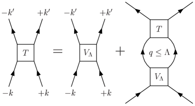
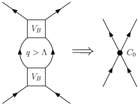
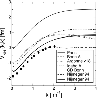
Figure 1: Left: Equation for the $T$-matrix with cut-off potential $V_{\Lambda}$ and replacement of the effects of high $q$ states with a contact interaction. Right: $\chi^{2}/\mbox{dof}\approx 1$ potentials in ${}^{1}S_{0}$ channel and corresponding $V_{\Lambda}(k,k)$’s at $\Lambda=2.1\,\mbox{fm}^{-1}$ (black dots) [2].

We can cut off the intermediate states at successively lower $\Lambda$; with each step we have to change the potential $V_{\Lambda}$ to maintain the same phase shifts. This determines a renormalization group (RG) equation for $V_{\Lambda}$ [2]. We see in Fig. 1 that at $\Lambda=2.1\,\mbox{fm}^{-1}$, corresponding to 350 MeV lab energy, the potentials have all collapsed to the same low-momentum potential (“$V_{{\rm low\,}k}$”). The net shifts are largely constant in momentum space, which means they are well represented by contact terms and a derivative expansion. This observation suggests a local Lagrangian approach. We also note that the high-momentum $\Lambda$ dependence for two-nucleon scattering appears as powers of $\Lambda$ only (no logarithms).

The low-energy data is insensitive to details of short-distance physics, so we can replace the latter with something simpler without distorting the low-energy physics. Effective field theory (EFT) is a local Lagrangian, model-independent approach to this program. Complete sets of operators at each order in an expansion permit systematic calculations with well-defined power counting. The program is realized as described in Ref. [1], which we apply to a basic many-body system, the dilute Fermi gas:

1. Use the most general Lagrangian with low-energy dof’s consistent with global and local symmetries of the underlying theory. For a dilute Fermi system, this takes the form (with omitted derivative and higher many-body terms):

   $${\cal L}_{\rm eft}=\psi^{\dagger}\bigl{[}i\frac{\partial}{\partial t}+\frac{\nabla^{\,2}}{2M}\bigr{]}\psi-\frac{{C_{0}}}{2}(\psi^{\dagger}\psi)^{2}-\frac{{D_{0}}}{6}(\psi^{\dagger}\psi)^{3}+\ldots$$ (1)

2. Declare a regularization and renormalization scheme. For a natural scattering length $a_{s}$ (e.g., hard spheres where $a_{s}\propto R$, the sphere radius), dimensional regularization and minimal subtraction (DR/MS) are particularly advantageous [3]. A simple matching to the effective range expansion for two-body scattering determines the two-body coefficients ($C_{i}$) to any desired order. For example, $C_{0}=4\pi a_{s}/M$.

3. Establish a well-defined power counting; e.g., the energy density ${\cal E}$ in powers of $k_{\scriptscriptstyle\rm F}a_{s}$:

   

    and so on. The rules yield

   $${\cal E}={\rho}\frac{{k_{\scriptscriptstyle\rm F}^{2}}}{2M}\biggl{[}\frac{3}{5}+{\frac{2}{3\pi}}{(k_{\scriptscriptstyle\rm F}a_{s})}+{\frac{4}{35\pi^{2}}(11-2\ln 2)}{(k_{\scriptscriptstyle\rm F}a_{s})^{2}}+\cdots\biggr{]}\ .$$ (2)

The calculation of the energy density is far easier in the EFT approach than in conventional treatments [3]. For example, each additional $C_{0}$ vertex simply brings a single power of $k_{\scriptscriptstyle\rm F}a_{s}$. The contribution for each diagram is a coefficient with all of the dependence on the short-range scale (e.g., $\Lambda\sim 1/R$) times a multi-dimensional integral that is simply a geometric factor (and which is conveniently evaluated even at high order using Monte Carlo integration).

2 Inevitability of Three-Body Interactions

Naively, it would appear from (2) that the energy density is a power series in $k_{\scriptscriptstyle\rm F}a_{s}$. In fact, the polynomial in $k_{\scriptscriptstyle\rm F}a_{s}$ is disrupted by three-body contributions. (The following contributions assume the spin/isospin degeneracy is greater than two.) These emerge inevitably in the form of logarithmic divergences in 3–to–3 scattering (left two diagrams):

$\stackrel{{\scriptstyle{\displaystyle\cal E}}}{{\Longrightarrow}}$ 

The divergence is easily isolated and in dimensional regularization the amplitude is

$${\cal T}_{3\to 3}^{\rm ln}=-iM^{3}(C_{0})^{4}\,\frac{4\pi-3\sqrt{3}}{8\pi^{3}}\Bigl{[}\frac{1}{D-3}-2\,{\ln\mu}+\cdots\Bigr{]}\ .$$ (3)

Changes in the parameter $\mu$ are absorbed by the three-body coupling $D_{0}(\mu)$, yielding an RG equation that is easily solved for the $\mu$ dependence of $D_{0}$ since $C_{0}$ is constant:

$$\mu\frac{d}{d\mu}D_{0}=M^{3}(C_{0})^{4}\,\frac{4\pi-3\sqrt{3}}{4\pi^{3}}\ \Longrightarrow\ D_{0}(\mu)=D_{0}(1/a_{s})+M^{3}(C_{0})^{4}\,\frac{4\pi-3\sqrt{3}}{4\pi^{3}}\,{\ln(a_{s}\mu)}\,.$$ (4)

The $\ln(\mu)$ dependence from $D_{0}(\mu)$ in the energy (fourth diagram) must be canceled, which tells us for free there is a term in the energy density proportional to $\ln(k_{\scriptscriptstyle\rm F}a_{s})$ with the same coefficient as the $\ln(a_{s}\mu)$ term in Eq. (4) [see Ref. [3] for the complete details]. While the logarithm is determined, $D_{0}(1/a_{s})$ is not: two-body data alone is insufficient!

We can further exploit the general structure of the renormalization group equations to identify additional logarithms (and powers of logarithms) [4, 3]. The scale $\mu$ only appears in logarithms, which means that matching $\Lambda$ dimensions in the RG equations is very restrictive. The couplings have dimension $C_{2i}\sim 4\pi/M\Lambda^{2i+1}$ and $D_{2i}\sim 4\pi/M\Lambda^{2i+4}$, so the RG equation for the coefficient $C_{0}(\mu)$ can only have one $C_{0}$ on the right side, which in turns tells us to look for log divergences in 2–to–2 diagrams with a single $C_{0}$:

$$\mu\frac{d}{d\mu}C_{0}=a\,C_{0}\ \Longrightarrow\ \mbox{tree-level only; no log divergence}\ \Longrightarrow\ a=0\ \Longrightarrow\ C_{0}=\mbox{const.}$$ (5)

For the three-body, no-derivative coefficient $D_{0}(\mu)$, we reproduce the form found above:

$$\mu\frac{d}{d\mu}D_{0} \!\!=\!\! a\,(C_{0})^{4}+b\,C_{0}C_{2}+c\,C_{0}C_{2}^{\prime}+dD_{0}\ \Longrightarrow\ b=0,\ c=0,\ d=0\ \mbox{(3--to--3 tree level)}$$ (6)

$$\Longrightarrow\ \frac{dD_{0}}{d\ln\mu}=a(C_{0})^{4}\ \Longrightarrow\ D_{0}(\mu)=a(C_{0})^{4}\ln\mu+{const.}$$

If the right side has $D_{0}\propto\ln\mu$, then the coefficient goes like $(\ln\mu)^{2}$, and so on [4].

3 Observables

An example of how subtle model dependence is clearly identified by the EFT arises when considering occupation numbers, which are typically treated as many-body observables. In a uniform system with second-quantized creation and destruction operators $a_{\bf k}^{\dagger}$ and $a_{\bf k}^{\phantom{\dagger}}$, the momentum (occupation) distribution is $n(k)=\langle a_{\bf k}^{\dagger}a_{\bf k}^{\phantom{\dagger}}\rangle$, which measures the strength of correlations (Fig. 2, left). It is said to be measurable in $(e,e^{\prime}p)$ on a nucleus. But is $n(k)$ an observable?

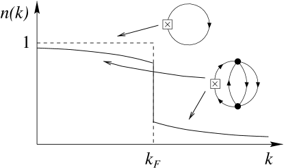
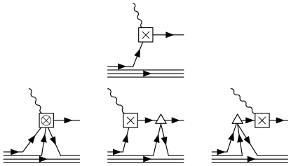
Figure 2: Left: Diagrammatic momentum distribution. Right: Schematic $(e,e^{\prime}p)$ process.

The status of potential observables can be tested using local field redefinitions, such as $\psi\longrightarrow\psi+\alpha(4\pi/{\Lambda^{3}})(\psi^{\dagger}\psi)\psi$ with arbitrary $\alpha$; if $\alpha\sim{\cal O}(1)$ this is “natural” [5]. (These field redefinitions are analogous to, but not the same as, unitary transformations.) Such a redefinition induces both two-body off-shell vertices (triangles) and three-body vertices. It can be shown that the energy density is model independent (i.e., independent of $\alpha$) if all terms are kept [5]:
                      

In this example, the one-body kinetic term generates the triangle vertex under the redefinition while the two-body no-derivative term generates the three-body vertex (open circle). If the three-body terms are omitted, then the energy would depend on $\alpha$ (even though the different forces reproduce the same two-body phase shifts) and then one might be fooled into thinking that $\alpha$ can be determined by comparison to experiment. The energies for different $\alpha$’s would lie along a “Coester line,” which is just a form of model dependence (“off-shell ambiguities”) made manifest by the EFT [5].

There are similar induced contributions to the momentum distribution, with the additional issue that the corresponding operator is changed by redefinitions and there is no preferred definition (there is no Noether current, as for the fermion number) [6]. These induced contributions correct the impulse approximation when analyzing $(e,e^{\prime}p)$ experiments, mixing vertex corrections (exchange currents) and initial and final state interactions in an $\alpha$-dependent way (see Fig. 2 right). This means that the distribution $n(k)$ is not directly accessible; more generally, experiment cannot resolve ambiguities in momentum distributions within a calculational framework based on low-energy degrees of freedom. Instead the distributions are auxiliary quantities defined only in a specific convention; they are useful within this convention but are not observables (this is analogous to quark distributions in deep inelastic scattering). However, the ambiguities have a natural size [6]; if they are negligible then the momentum distributions are effectively observables.

4 Current Trends in Many-Body EFT

The EFT tools and techniques offer many new possibilities for the systematic and model-independent calculation of many-body systems; the examples here involving three-body interactions are just a sampler. When contributions to three- and higher-body scattering from multiple short-distance two-body scatterings have logarithmic divergences at large intermediate-state momentum, they are not resolved and three-body interactions must be included to avoid model dependence. Careful consideration of the regulator dependence turns a necessity into a virtue, providing valuable information about the analytic structure of observables. The second example illustrated how local field redefinitions are a clean tool for assessing potential observables. Simple rule: if a calculated quantity depends on a transformation parameter $\alpha$, it is either not an observable or you’ve forgotten some contribution. These transformations also demonstrate explicitly how different two-body forces are associated with different three-body forces.

Other topics under current investigation include nonperturbative EFT and applications to finite systems. The effective action formalism has been used for a nonperturbative large N expansion in Ref. [7] and work is in progress to extend the EFT approach to large $a_{s}$ that was initiated by Steele [8]. A merger of density functional theory (DFT) and EFT is presented in Ref. [9], with on-going work on long-range forces, pairing, and a systematic gradient expansion. Some planned applications are energy functionals for nuclei far from stability and superfluidity in trapped fermionic atoms. Other groups are adapting chiral perturbation theory to many-body systems [1] and there is an EFT program for bosonic systems by Braaten, Hammer, and collaborators [10].

References

- [1] S. R. Beane et al., “From Hadrons to Nuclei: Crossing the Border,” nucl-th/0008064 and references therein.
- [2] S. K. Bogner, T. T. Kuo and A. Schwenk, nucl-th/0305035.
- [3] H.-W. Hammer and R. J. Furnstahl, Nucl. Phys. A678 (2000) 277.
- [4] E. Braaten and A. Nieto, Phys. Rev. B 55 (1997) 8090; 56 (1997) 14745.
- [5] R. J. Furnstahl, H.-W. Hammer, and N. Tirfessa, Nucl. Phys. A689 (2001) 846.
- [6] R. J. Furnstahl and H.-W. Hammer, Phys. Lett. B 531 (2002) 203.
- [7] R. J. Furnstahl and H.-W. Hammer, Ann. Phys. (NY) 302 (2002) 206.
- [8] J. Steele, nucl-th/0010066.
- [9] S. Puglia, A. Bhattacharyya, and R. J. Furnstahl, Nucl. Phys. A723 (2003) 145.
- [10] E. Braaten, H.-W. Hammer, cond-mat/0303249 and references therein.