Dressed vertices

Abstract

The response of a correlated nuclear system to an external field is discussed. The Bethe-Salpeter equation for the dressed vertex is solved. The kernel of the integral equation for the vertex is chosen consistently with the approximation for the self-energy. This guarantees the fulfillment of the f-sum rule for the response function.

sum rules, vertex corrections, nuclear matter

21.65.+f, 24.10.Cn, 26.60.+c

Processes occurring in dense nuclear matter are modified by the effects of the medium. This happens for neutrino rates in neutron stars [1, 2, 3, 4, 5, 6, 7] and for particle or photon emission in hot nuclear matter [8, 9, 10, 11, 12]. In particular the effect of the off-shell propagation of nucleons in the medium is important for the subthreshold particle production in heavy ion collisions. The role of correlations for the neutrino emission could be especially important for processes in hot stars. Soft particle emission is influenced by the multiple scattering in the medium, which is equivalent to including vertex correction modifying the coupling of the external current to the dressed nucleons [13]. In-medium modifications of the vertex cannot be described only as modification of the coupling constant. The three-point function describing the modified coupling of the external current to the fermions in medium has a complicated analytical structure and depends on the incoming momenta and energies [14, 15].

For the case of weak coupling of the external current or of the produced particles to the nucleons, the problem is equivalent to the calculation of the response function in the correlated medium. For the Hartree-Fock approximation the response function can be calculated from the random-phase approximation, which however is usually taken at the ring diagrams level only. The use of advanced approximations for the description of the many-particle system with in-medium propagators dressed by the interaction and scattering, raises the question of the correct treatment of the vertex corrections [16]. It is known that the density response function for the electron gas in the self-consistent GW approximation [17] violates the f-sum rule [18, 19]. For a given approximation for the self-energy the corresponding vertex corrections can be obtained by solving the Bethe-Salpeter equation with a specific particle-hole irreducible kernel [20, 16]. The actual solution of the integral equation for the in-medium vertex is quite complex, a complete solution for dressed propagators was given by Kwong and Bonitz [21] from the solution of non-equilibrium Kadanoff-Baym equations in an external field. This procedure is numerically quite involved. The initial state is given by a non-equilibrium evolution of the quantum transport equations and is not easy to tune. For a quantum well the equations for the dressed vertex were solved using equilibrium Green’s function technique taking the most important part of the particle-hole irreducible kernel [22]. Below we present the first solution of the Bethe-Salpeter equation for the dressed vertex in a nuclear system for a general momentum and energy of the external field coupled to the density using the real-time Green’s function formalism.

Self-consistent approximations for nuclear systems include iterated second Born approximation using an effective interaction [23, 9, 10] and in medium T-matrix calculations using free nucleon-nucleon interactions [24, 25, 26]. These schemes use dressed nucleons with nontrivial spectral functions and the response function cannot be obtained simply by calculating the particle-hole polarization loop. The dressed vertex describing the coupling of the external current to the in-medium nucleons is given by a Bethe-Salpeter equation (Fig. 1), where $K$ denotes the particle-hole irreducible kernel. For a self-consistent approximation to the self-energy one should take for the kernel $K$ the functional derivative of the self-energy with respect to the dressed Green’s function [20, 16] $K={\delta\Sigma}/{\delta G}$.

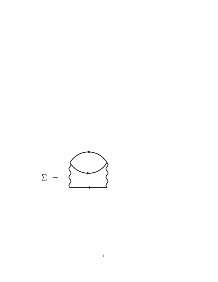
Figure 2: The self-energy in the Born approximation.

In the following we use the self-consistent second Born approximation with the effective interaction taken from [23] (Fig. 2). The solution of the self-consistent equations for the self-energy and dressed propagators in equilibrium is standard [9, 27, 10] and numerical easy to implement. In the real time formalism the nucleon retarded (advanced) Green’s function is expressed by the retarded (advanced) self-energy $\Sigma^{r(a)}$ through the Dyson equation

$$G^{r(a)}({\bf p},\omega)=\frac{1}{\omega-{\bf p}^{2}/2m-\Sigma^{r(a)}({\bf p},\omega)}\ .$$ (1)

The self-energy is taken in the second direct Born approximation

$$\Sigma^{>(<)}({\bf p},\omega) = 4i\int\frac{d^{3}p_{1}d\omega_{1}d^{3}p_{2}d\omega_{2}}{(2\pi)^{8}}V^{2}({\bf p}-{\bf p_{1}})G^{>(<)}({\bf p_{1}},\omega_{1})G^{<(>)}({\bf p_{2}},\omega_{2})$$ (2)

$$G^{>(<)}({\bf p}-{\bf p_{1}}+{\bf p_{2}},\omega-\omega_{1}+\omega_{2})\ ,$$

where the Green’s functions

$$G^{>}({\bf p},\omega) = -i\left(1-f(\omega)\right)A({\bf p},\omega)$$

$$G^{<}({\bf p},\omega) = if(\omega)A({\bf p},\omega)$$ (3)

are written using the Fermi distribution $f(\omega)$ and the spectral function

$$A({\bf p},\omega)=-2{\rm Im}G^{r}({\bf p},\omega)\ ,$$ (4)

also

$$\Sigma^{r(a)}({\bf p},\omega)=\int\frac{d\omega_{1}}{2\pi}\frac{\Sigma^{<}({\bf p},\omega_{1})-\Sigma^{>}({\bf p},\omega_{1})}{\omega-\omega_{1}\pm i\epsilon}\ .$$ (5)

Equations (1), (2) and (4) are solved by iteration with a constraint on the total density of the system. In the following we present results for the density $\rho=0.32$fm^-3 and the temperature of $5$MeV. The single-particle width is of about $20-30$MeV. The polarization bubble without vertex corrections is given by

$$\Pi^{<(>)}({\bf q},\Omega)=-4i\int\frac{d^{3}pd\omega}{(2\pi)^{4}}G^{<(>)}({\bf q}+{\bf p},\omega+\Omega)G^{>(<)}({\bf p},\omega)\ .$$ (6)

The retarded and advanced polarization $\Pi^{r(a)}$ can be obtained using a dispersion relation from its imaginary part $2{\rm Im}\Pi^{r}=\Pi^{>}-\Pi^{<}$.

Let us define the Green’s function in a weak external field of momentum $q$ and energy $\Omega$ coupled to the density. For the incoming nucleon momentum ${\bf p}$ and energy $\omega$ the outgoing momentum is ${\bf q}+{\bf p}$ and the energy $\omega+\Omega$. We define the smaller (larger) Green’s functions

$$G_{I}^{<(>)}({\bf q}+{\bf p},\omega+\Omega;{\bf p},\omega)$$ (7)

and the retarded (advanced) Green’s functions

$$G_{I}^{r(a)}({\bf q}+{\bf p},\omega+\Omega;{\bf p},\omega)\ ,$$ (8)

with respect to the ordering of the fermion legs in the three-point function $G_{I}$, the dependence on the external energy $\Omega$ corresponds always to a retarded vertex. They fulfill the relation

$$G_{I}^{r}-G_{I}^{a}=G_{I}^{>}-G_{I}^{<}$$ (9)

but there is no spectral representation for them. It means that there are three independent Green’s functions $G_{I}$ as expected [28]. The Green’s functions $G_{I}$ are given by the amputated vertex $\Gamma$

$$G_{I}^{r(a)}({\bf q}+{\bf p},\omega+\Omega;{\bf p},\omega)=G^{r(a)}({\bf q}+{\bf p},\omega+\Omega)\Gamma^{r(a)}({\bf q}+{\bf p},\omega+\Omega;{\bf p},\omega)G^{r(a)}({\bf p},\omega)$$ (10)

and

$$G_{I}^{<(>)}({\bf q}+{\bf p},\omega+\Omega;{\bf p},\omega)=G^{r}({\bf q}+{\bf p},\omega+\Omega)\Gamma^{r}({\bf q}+{\bf p},\omega+\Omega;{\bf p},\omega)G^{<(>)}({\bf p},\omega)$$

$$+G^{r}({\bf q}+{\bf p},\omega+\Omega)\Gamma^{<(>)}({\bf q}+{\bf p},\omega+\Omega;{\bf p},\omega)G^{a}({\bf p},\omega)$$

$$+G^{<(>)}({\bf q}+{\bf p},\omega+\Omega)\Gamma^{a}({\bf q}+{\bf p},\omega+\Omega;{\bf p},\omega)G^{a}({\bf p},\omega)\ .$$ (11)

The dressed vertex $\Gamma$ for the coupling of the external field to the nucleon is the solution of the Bethe-Salpeter equation. The particle-hole irreducible kernel for the self-energy given by Eq. (2) is shown in Fig. 3.

Defining the polarization bubble coupled to the external field

$$\Pi_{I}^{<(>)}({\bf q}+{\bf p},\omega+\Omega;{\bf p},\omega)=-4i\int\frac{d^{3}p_{1}d\omega_{1}}{(2\pi)^{4}}\left(G_{I}^{<(>)}({\bf q}+{\bf p}+{\bf p_{1}},\omega+\Omega+\omega_{1};{\bf p}+{\bf p_{1}},\omega+\omega_{1})\right.$$

$$\left.G^{>(<)}({\bf p_{1}},\omega_{1})+G^{<(>)}({\bf p}+{\bf p_{1}},\omega+\omega_{1})G_{I}^{>(<)}({\bf p_{1}},\omega_{1};{\bf p_{1}}-{\bf q},\omega_{1}-\Omega)\right)$$ (12)

and

$$\Pi_{I}^{r(a)}({\bf q}+{\bf p},\omega+\Omega;p,\omega)=-4i\int\frac{d^{3}p_{1}d\omega_{1}}{(2\pi)^{4}}\left(G_{I}^{r(a)}({\bf q}+{\bf p}+{\bf p_{1}},\omega+\Omega+\omega_{1};{\bf p}+{\bf p_{1}},\omega+\omega_{1})\right.$$

$$G^{<(>)}({\bf p_{1}},\omega_{1})+G^{r(a)}({\bf p}+{\bf p_{1}},\omega+\omega_{1})G_{I}^{<(>)}({\bf p_{1}},\omega_{1};{\bf p_{1}}-{\bf q},\omega_{1}-\Omega)$$

$$+G_{I}^{<(>)}({\bf q}+{\bf p}+{\bf p_{1}},\omega+\Omega+\omega_{1};{\bf p}+{\bf p_{1}},\omega+\omega_{1})G^{r(a)}({\bf p_{1}},\omega_{1})$$

$$\left.+G^{<(>)}({\bf p}+{\bf p_{1}},\omega+\omega_{1})G_{I}^{r(a)}({\bf p_{1}},\omega_{1};{\bf p_{1}}-{\bf q},\omega_{1}-\Omega)\right)$$ (13)

we can write the Bethe-Salpeter equations for the dressed vertex as

$$\Gamma^{<(>)}({\bf p}+{\bf q},\omega+\Omega;{\bf p},\omega)=i\int\frac{d^{3}p_{1}d\omega_{1}}{(2\pi)^{4}}\left(V^{2}({\bf p}-{\bf p_{1}})\Pi^{<(>)}({\bf p}-{\bf p_{1}},\omega-\omega_{1})\right.$$

$$G_{I}^{<(>)}({\bf p_{1}}+{\bf q},\omega_{1}+\Omega;{\bf p_{1}},\omega_{1})$$

$$\left.+V({\bf p_{1}})V({\bf p_{1}}+{\bf q})\Pi_{I}^{<(>)}({\bf p_{1}}+{\bf q},\omega_{1}+\Omega;{\bf p_{1}},\omega_{1})G^{<(>)}({\bf p}-{\bf p_{1}},\omega-\omega_{1})\right)$$ (14)

and

$$\Gamma^{r(a)}({\bf p}+{\bf q},\omega+\Omega;{\bf p},\omega)=1+i\int\frac{d^{3}p_{1}d\omega_{1}}{(2\pi)^{4}}\left(V^{2}({\bf p}-{\bf p_{1}})\Pi^{<}({\bf p}-{\bf p_{1}},\omega-\omega_{1})\right.$$

$$G_{I}^{r(a)}({\bf p_{1}}+{\bf q},\omega_{1}+\Omega;{\bf p_{1}},\omega_{1})$$

$$+V({\bf p_{1}})V({\bf p_{1}}+{\bf q})\Pi_{I}^{<}({\bf p_{1}}+{\bf q},\omega_{1}+\Omega;{\bf p_{1}},\omega_{1})G^{r(a)}({\bf p}-{\bf p_{1}},\omega-\omega_{1})$$

$$+V^{2}({\bf p}-{\bf p_{1}})\Pi^{r(a)}({\bf p}-{\bf p_{1}},\omega-\omega_{1})G_{I}^{>}({\bf p_{1}}+{\bf q},\omega_{1}+\Omega;{\bf p_{1}},\omega_{1})$$

$$\left.+V({\bf p_{1}})V({\bf p_{1}}+{\bf q})\Pi_{I}^{r(a)}({\bf p_{1}}+{\bf q},\omega_{1}+\Omega;{\bf p_{1}},\omega_{1})G^{>}({\bf p}-{\bf p_{1}},\omega-\omega_{1})\right)\ .$$ (15)

The equations for the dressed vertex (Dressed vertices), (Dressed vertices) and for Green’s function in the external field (10), (Dressed vertices) are iterated for each given $q$ and $\Omega$, using the Green’s functions $G$ obtained for the correlated system in equilibrium. The irreducible polarization bubble including vertex corrections for the density response is calculated from the Green’s function $G_{I}^{<}$

$$\Pi_{irr}^{r}({\bf q},\Omega)=-4i\int\frac{d^{3}pd\omega}{(2\pi)^{4}}G_{I}^{<}({\bf p}+{\bf q},\omega+\Omega;{\bf p},\omega)\ .$$ (16)

In Fig. 4 is show the polarization bubble with vertex corrections $\Pi_{irr}$ for $q=220$MeV. The result is very different from the naive one-loop polarization (6), the vertex corrections are very important. The response function is closer to the response of a noninteracting system, but not exactly the same. We have made a calculation of the polarization function neglecting the contributions of the terms with $\Pi_{I}$ in the Bethe-Salpeter equations (Dressed vertices), (Dressed vertices). This corresponds to neglecting the last two diagrams in the particle-hole kernel (Fig. 3). The result is different which shows that the full kernel of the Bethe-Salpeter equation must be taken and not only the first term in Fig. 3.

Unlike for the function $G_{I}$, the real and imaginary parts of the polarization bubble $\Pi_{irr}^{r}$ fulfill a dispersion relation

$${\rm Re}\Pi_{irr}^{r}({\bf q},\omega)=-\int\frac{d\omega_{1}}{\pi}\frac{{\rm Im}\Pi_{irr}^{r}({\bf q},\omega_{1})}{\omega-\omega_{1}+i\epsilon}\ .$$ (17)

The dispersion relations between the independently obtained real and imaginary parts of the response function constitutes a useful check of the consistency of the approach and of the numerics. Another important consistency of the response functions is given by the f-sum rule

$$-\int\frac{\omega d\omega}{2\pi}{\rm Im}\Pi_{irr}^{r}({\bf q},\omega)=\rho\frac{{\bf q}^{2}}{2m}\ .$$ (18)

The above sum rule is well satisfied for the free response and for the response function including vertex corrections, it is severely violated for the naive polarization loop with dressed propagators (6). Please note that the sum rule is satisfied also by the solution using a simplified kernel in the Bethe-Salpeter equation, although the polarization itself is quite different. Our numerical method is quite accurate for $q>100$MeV, where both the f-sum rule and the dispersion relation (17) are satisfied. Note that in the region where the calculations are performed the vertex corrections are still very important, essential in guaranteeing the fulfillment of the sum rule. For example at $q=220$MeV the naive polarization loop with dressed propagators violates the sum rule by a factor 4.9 .

Adding the Hartree-Fock terms in the self-energy modifies the kernel of the equation for the dressed vertex. The Fock term generates an additional interaction line in Fig. 3, the exchange term in the random-phase approximation. The Hartree term generates the ring series which is summed to give the polarization

$$\frac{\Pi^{r}_{irr}({\bf q},\Omega)}{1-V({\bf q})\Pi^{r}_{irr}({\bf q},\Omega)}\ .$$ (19)

We have checked that adding at the same time a Hartree-Fock term to the self-energy (2) and an exchange interaction ladder in the kernel of the Bethe-Salpeter equation conserves the sum rule for $\Pi_{irr}^{r}$. This sum rule is then conserved after performing the ring summation (19), although the shape of the response function itself is strongly modified by the transformation (19). The irreducible response function with vertex correction is close to the noninteracting one, however after the ring summation the results are different due to a different tail in ${\rm Im}\Pi_{irr}$ at large energies. The study of the full response with a realistic effective Hartree-Fock self-energy will be presented elsewhere.

We present a solution of the Bethe-Salpeter equation for the vertex of the external field coupled to the density in a correlated medium. The approximation chosen for the particle-hole interaction is consistent with the nontrivial self-energy used in the Dyson equation. It guarantees the fulfillment of the f-sum rule for the response function. To our knowledge it is the first solution of the Bethe-Salpeter equation for a general momentum and energy, using equilibrium Green’s function formalism and the full kernel of the integral equation for the dressed vertex. The irreducible polarization with vertex corrections is much closer to the Lindhard function than the naive one loop polarization with dressed propagators. It is a manifestation of the expected cancellation of the self-energy and vertex corrections. The methods here presented can be used to calculate realistic response functions with different vertices or to test approximations for the dressed vertices or for the particle-hole interaction for the more complicated T-matrix self-energies in nuclear matter.

Acknowledgments This work was partly supported by the KBN under Grant No. 2P03B05925.

Figure 1: The Bethe-Salpeter equation for the dressed vertex. The particle-hole irreducible kernel $K$ is denoted by the box and the fat and the small dots denote the dressed and the bare vertices respectively.

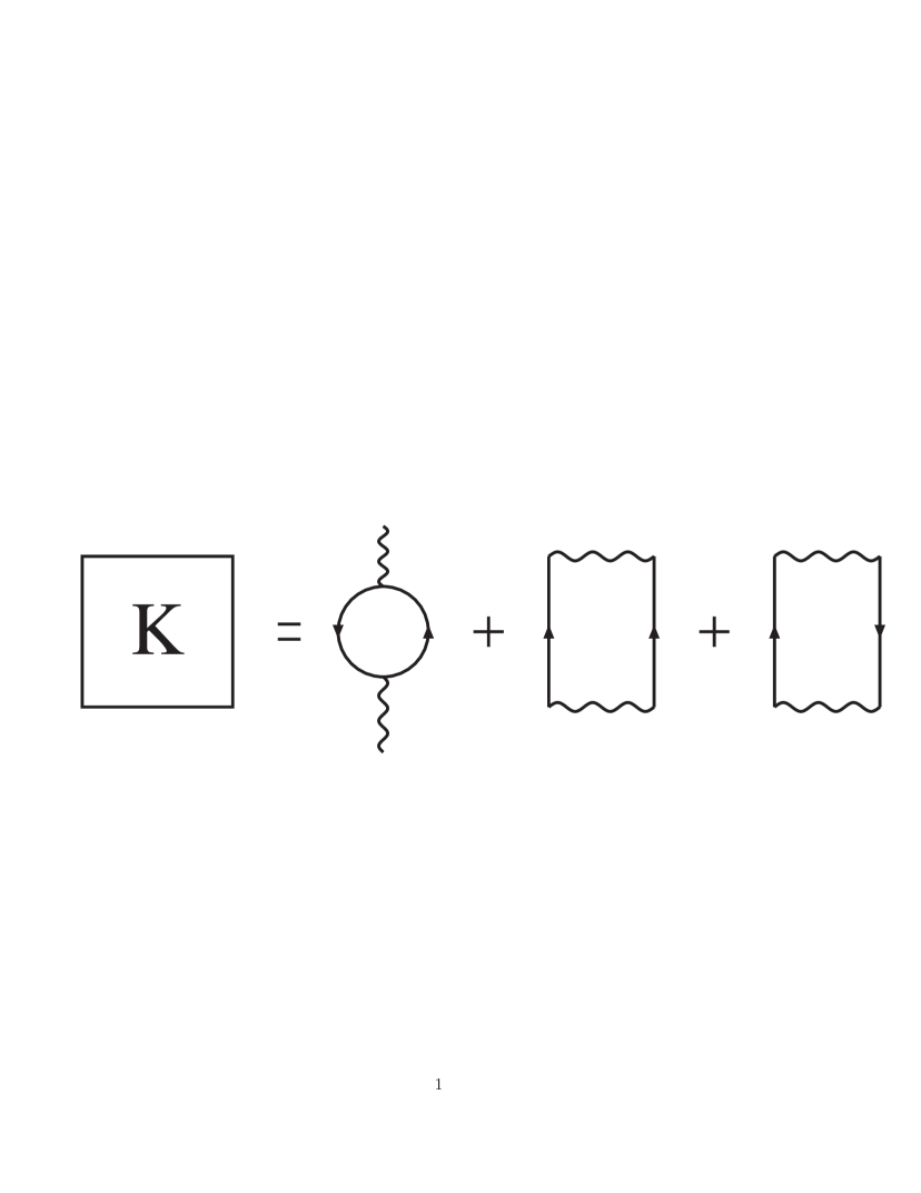
Figure 3: The particle-hole irreducible vertex corresponding to the self-energy in Fig. 2.

Figure 4: The imaginary part of the irreducible polarization as function of the energy for $q=220$MeV. The solid line denotes the result with vertex corrections, the dotted line is the one-loop calculation with dressed propagators (Eq. 6), and the dashed line is the polarization for the noninteracting system. The dashed-dotted line denotes the polarization with vertex corrections restricted only to the first diagram in Fig. 3.

Figure 5: The ratio of the f-sum rule to the expected value as function of the momentum in the response function. The lines are the same as in Fig. 4.

References

- [1] B. Friman, O. Maxwell, Astophys. J., 232 (1979) 541.
- [2] S. Reddy, M. Prakash, J. Lattimer, J. Pons, Phys. Rev., C59 (1998) 2888.
- [3] D. Yakovlev, A. Kaminker, O. Gnedin, P. Haensel, Phys. Rep., 354 (2001) 1.
- [4] D. Voskresensky, A. Senatorov, Sov. Phys. JETP, 63 (1986) 885.
- [5] S. Yamada, H. Toki, Phys. Rev., C61 (1999) 015803.
- [6] G. Raffelt, D. Seckel, Phys. Rev. Lett., 67 (1991) 2605.
- [7] A. Sedrakian, A. Dieperink, Phys. Rev., D62 (2000) 083002.
- [8] P. Bożek, Phys. Rev., C56 (1997) 1452.
- [9] P. Bożek, in: K. Morawetz, P. Lipavský, V. Špička (Eds.), 5th Workshop on Nonequilibrium Physics at Short Time Scales, Universität Rostock, Rostock, 1998.
- [10] M. Effenberger, U. Mosel, Phys. Rev., C60 (1999) 051901.
- [11] W. Cassing, S. Juchem, Nucl. Phys., A677 (2000) 445–460.
- [12] G. F. Bertsch, P. Danielewicz, Phys. Lett., B367 (1996) 55–59.
- [13] J. Knoll, D. N. Voskresensky, Annals Phys., 249 (1996) 532.
- [14] G. D. Mahan, Many-Particle Physics, Plenum, New York, 1990.
- [15] T. S. Evans, Phys. Lett., B249 (1990) 286.
- [16] J. Blaizot, G. Ripka, Quantum Theory Of Finite Systems, MIT Press, Cambridge, 1986.
- [17] F. Aryasetiawan, O. Gunnarsson, Rep. Prog. Phys., 61 (1998) 237.
- [18] A. Schindlmayr, R. Godby, Phys. Rev. Lett., 80 (1998) 1702.
- [19] D. Tamme, R. Schepe, K. Henneberger, Phys. Rev. Lett., 83 (1999) 241.
- [20] G. Baym, L. Kadanoff, Phys. Rev., 124 (1961) 287.
- [21] N. Kwong, M. Bonitz, Phys. Rev. Lett., 84 (2000) 1768.
- [22] S. Faleev, M. Stockman, Phys. Rev., B66 (2002) 085318.
- [23] P. Danielewicz, Annals Phys., 152 (1984) 305.
- [24] P. Bożek, Phys. Rev., C65 (2002) 054306.
- [25] Y. Dewulf, W. H. Dickhoff, D. Van Neck, E. R. Stoddard, M. Waroquier, Phys. Rev. Lett., 90 (2003) 152501.
- [26] T. Frick, H. Müther, nucl-th/0306009.
- [27] J. Lehr, M. Effenberger, H. Lenske, S. Leupold, U. Mosel, Phys. Lett., B483 (2000) 324–330.
- [28] D. Hou, E. Wang, U. Heinz, J. Phys., G24 (1998) 1861.