On meson resonances and chiral symmetry

Abstract

We study meson resonances with quantum numbers $J^{P}=1^{+}$ in terms of the chiral SU(3) Lagrangian. At leading order a parameter-free prediction is obtained for the scattering of Goldstone bosons off vector mesons with $J^{P}=1^{-}$ once we insist on approximate crossing symmetry of the unitarized scattering amplitude. A resonance spectrum arises that is remarkably close to the empirical pattern. In particular, we find that the strangeness-zero resonances $h_{1}(1380)$, $f_{1}(1285)$ and $b_{1}(1235)$ are formed due to strong $K\,\bar{K}_{\mu}$ and $\bar{K}\,K_{\mu}$ channels. This leads to large coupling constants of those resonances to the latter states.

GSI-Preprint-2003-19

1 Introduction

In recent works [1, 2, 3, 4, 5] it was demonstrated that chiral SU(3) symmetry predicts parameter-free $J^{P}\!=\!\frac{1}{2}^{-}$ and $J^{P}\!=\!\frac{3}{2}^{-}$ baryon resonances. It was observed that the resonance states turn into bound states in the heavy SU(3) limit with $m_{\pi,K,\eta}\simeq 500$ MeV but disappear altogether in the light SU(3) limit with $m_{\pi,K,\eta}\simeq 140$ MeV. Related works [6, 7, 8, 9, 10] that did not insist on approximate crossing symmetric scattering amplitudes [3] and therefore involve a larger set of free parameters adjusted to the data are in qualitative agreement with the parameter-free computation [4] for the s-wave $J^{P}\!=\!\frac{1}{2}^{-}$ baryon resonances. Even earlier in the 60s a series of works [11, 12, 13, 14, 15] predicted a wealth of s-wave baryon resonance generated by coupled-channel dynamics. Those works were based on a SU(3)-symmetric interaction Lagrangian that is closely related to the leading order chiral Lagrangian. All these results strongly support a conjecture put forward by the authors that baryon resonances that do not belong to the large-$N_{c}$ ground state of QCD are generated by coupled-channel dynamics [2, 3, 16]. If this conjecture is further substantiated one would expect an analogous mechanism to be at work in the meson sector, i.e. we conjecture in this work that meson resonances not belonging to the large-$N_{c}$ ground state of QCD are generated by coupled-channel dynamics as well. In contrast to the baryon sector it is not so immediate which meson states one should identify to be the large-$N_{c}$ ground states of QCD. Without controversy we would take for the latter the SU(3) Goldstone bosons, ($\pi(140),K(494),\eta(545)$), with $J^{P}\!=\!0^{-}$ and the lightest vector mesons ($\rho_{\mu}(770),\omega_{\mu}(782),K_{\mu}(892),\phi_{\mu}(1020)$) with $J^{P}\!=\!1^{-}$. However, it is unclear whether to include also the lightest meson resonances with quantum numbers $J^{P}\!=\!0^{+}$ and $J^{P}\!=\!1^{+}$. From recent coupled-channel analyses that were based on the chiral SU(3) Lagrangian and were able to quantitatively describe the $\pi\pi$ phase shifts in the $J^{P}\!=\!0^{+}$ sector we would conclude that meson resonances with scalar quantum numbers should be generated dynamically. A prime example is the $f_{0}(980)$ resonance [17, 18, 19, 20, 21, 22] which long ago was found to be a $K\bar{K}-$molecule. This is analogous to the finding that the parity partners of the large-$N_{c}$ baryon ground states, i.e. baryon resonances with $J^{P}\!=\!\frac{1}{2}^{-}$ and $J^{P}\!=\!\frac{3}{2}^{-}$, are predicted by chiral coupled-channel dynamics. In view of these results it is quite natural to also describe the axial-vector meson resonances in terms of coupled-channel dynamics rather than identifying the latter to be part of the large-$N_{c}$ ground state of QCD. Our point of view differs here from that one expressed in recent works [23, 24] where the axial-vector mesons are part of a minimal hadronic ansatz of large-$N_{c}$ QCD.

In this work we study the scattering of Goldstone bosons off vector mesons using the leading order chiral Lagrangian. Our results are parameter free once we insist on approximate crossing symmetric scattering amplitudes. We find that chiral symmetry predicts the existence of the axial-vector meson resonances ($h_{1}(1170),h_{1}(1380),f_{1}(1285),a_{1}(1260),b_{1}(1235),K_{1}(1270),K_{1}(1400)$) with a spectrum that is surprisingly close to the empirical one. A result analogous to the baryon sector [3, 4, 5] is found: in the heavy SU(3) limit with $m_{\pi,K,\eta}\simeq 500$ MeV and $m_{\rho,\omega,K^{*},\phi}\simeq 900$ MeV the resonance states turn into bound states forming two degenerate octets and one singlet of the SU(3) flavor group with masses 1360 MeV and 1280 MeV respectively. Taking the light SU(3) limit with $m_{\pi,K,\eta}\simeq 140$ MeV and $m_{\rho,\omega,K^{*},\phi}\simeq 700$ MeV we do not observe any bound-state nor resonance signals anymore. Since the leading order interaction kernel scales with $N_{c}^{-1}$ the resonances disappear also in large-$N_{c}$ limit. Using physical masses a pattern arises that compares surprisingly well with the empirical properties of the $J^{P}\!=\!1^{-}$ meson resonances.

2 Chiral coupled-channel dynamics: the $\chi$-BS(3) approach

The starting point to study the scattering of Goldstone bosons off vector mesons is the chiral SU(3) Lagrangian. Though it is straight forward to construct the infinite tower of covariant interaction terms [25] the inclusion of massive vector mesons into the chiral Lagrangian is non-trivial: it requires a careful check whether chiral power counting rules can be realized manifestly. A solution to this problem is a systematic heavy-meson expansion [27]. An alternative solution is offered by the minimal chiral $\overline{MS}_{\chi}$-scheme [3] developed in the meson-baryon sector recently (see also [28, 29, 30]). The latter is based on dimensional regularization as applied to Feynman diagrams derived from the relativistic chiral Lagrangian and therefore preserves also all Ward identities if applied in perturbation theory. It exploits an ambiguity of how to introduce a subtraction scheme in dimensional regularization that arises once the theory is expected to be applicable only around a heavy mass scale. Certain algebraic consistency identities that probe the full relativistic loop functions outside the validity domain of the theory but that are respected by the $\overline{MS}$ scheme are given up with the benefit that chiral power counting rules can be implemented manifestly. Consistency is achieved by subtracting not only the standard poles at $d=4$ but in addition poles at $d=3$ [31] that arise in the chiral limit. The resulting loop functions are finite and well defined and comply with the leading chiral moment predicted by chiral power counting rules. The loop functions may be expanded further identifying subleading chiral moments. It is obvious that the $\overline{MS}_{\chi}$ scheme is applicable to the chiral Lagrangian involving any heavy fermion or boson field.

We proceed and identify the leading order Weinberg-Tomozawa interaction Lagrangian density [32, 25, 26]

$${\mathcal{L}}_{WT}(x) = -\frac{1}{16\,f^{2}}\,\rm tr\,\Big{(}[\Phi^{\mu}(x)\,,(\partial^{\nu}\Phi_{\mu}(x))]_{-}\,[\phi(x),(\partial_{\nu}\,\phi(x))]_{-}\Big{)}\,,$$ (1)

describing the interaction of the Goldstone bosons field $\phi$ with a massive vector-meson field $\Phi_{\mu}$. The parameter $f$ in (1) is known from the weak decay process of the pions. We use $f=90$ MeV through out this work. In (1) we omit additional terms that do not contribute to the on-shell scattering amplitude of Goldstone bosons off vector-meson at tree-level. Such terms are suppressed and not probed in a leading order calculation using the $\chi-$BS(3) scheme. Similarly we do not anticipate a dependence on the choice of the realization of the spin 1 field, though this issue may deserve further studies once sub-leading terms are included. Due to the on-shell reduction scheme discussed in detail in the following section we do not expect different results if we apply the tensor realization rather than the vector realization used in (1). The equivalence of the two realizations in some cases was demonstrated in [26] to leading orders.

Since we will assume perfect isospin symmetry it is convenient to decompose the fields into their isospin multiplet

$$\phi=\tau\cdot\pi(140)+\alpha^{\dagger}\cdot K(494)+K^{\dagger}(494)\cdot\alpha+\eta(547)\,\lambda_{8}\,,$$

$$\Phi_{\mu}=\tau\cdot\rho_{\mu}(770)+\alpha^{\dagger}\cdot K_{\mu}(892)+K_{\mu}^{\dagger}(892)\cdot\alpha$$

$$\qquad+\Big{(}{\textstyle{2\over 3}}+{\textstyle{1\over\sqrt{3}}}\,\lambda_{8}\Big{)}\,\omega_{\mu}(782)+\Big{(}{\textstyle{\sqrt{2}\over 3}}-\sqrt{{\textstyle{2\over 3}}}\,\lambda_{8}\Big{)}\,\phi_{\mu}(1020)\,,$$

$$\alpha^{\dagger}={\textstyle{1\over\sqrt{2}}}\,(\lambda_{4}+i\,\lambda_{5},\lambda_{6}+i\,\lambda_{7})\,,\qquad\tau=(\lambda_{1},\lambda_{2},\lambda_{3})\,,$$ (2)

with for instance $K_{\mu}=(K_{\mu}^{(+)},K^{(0)}_{\mu})^{t}$ and $\rho_{\mu}=(\rho_{\mu}^{(1)},\rho_{\mu}^{(2)},\rho_{\mu}^{(3)})$. The matrices $\lambda_{i}$ are the standard Gell-Mann generators of the SU(3) algebra. The numbers in the brackets recall the approximate masses of the fields in units of MeV.

As was emphasized in [3] the chiral SU(3) Lagrangian should not be used in perturbation theory except at energies sufficiently below all thresholds. Though the infinite set of irreducible diagrams can be successfully approximated by the standard perturbative chiral expansion that is no longer true for the infinite set of reducible diagrams once the energies are sufficiently large to support hadronic scattering processes. Whereas the former diagrams are controlled by the typical small parameter $m_{K}/(4\pi f)$ the latter ones probe a parameter of unit size $m_{K}^{2}/(8\pi f^{2})$, which invalidates any perturbative expansion. From an effective field theory point of view it is mandatory to sum the reducible diagrams. This is naturally achieved by considering the Bethe-Salpeter scattering equation,

$$T_{\mu\nu}(\bar{k},k;w)=K_{\mu\nu}(\bar{k},k;w)+\int\frac{d^{4}l}{(2\,\pi)^{4}}\,K_{\mu\beta}(\bar{k},l;w)\,G^{\alpha\beta}(l;w)\,T_{\alpha\nu}(l,k;w)\,,$$

$$G_{\mu\nu}(l;w)=\frac{i}{({\textstyle{1\over 2}}\,w-l)^{2}-m^{2}+i\,\epsilon}\,\frac{g_{\mu\nu}-({\textstyle{1\over 2}}\,w+l)_{\mu}\,({\textstyle{1\over 2}}\,w+l)_{\nu}/M^{2}}{({\textstyle{1\over 2}}\,w+l)^{2}-M^{2}+i\,\epsilon}\,,$$ (3)

where we suppress the coupled-channel structure for simplicity. We use physical values for the Goldstone boson and vector meson masses $m$ and $M$ respectively. Since the intermediate vector mesons have in part a substantial decay width we allow for spectral distributions of the broadest vector mesons, the $\rho_{\mu}$- and $K_{\mu}$-mesons. In channels involving the $\rho_{\mu}-$ or $K_{\mu}-$meson the two-particle propagator, $G$, in (3) is folded with spectral functions obtained at the one-loop level describing the decay processes $\rho_{\mu}\to\pi\,\pi$ and $K_{\mu}\to\pi\,K$.

$(0,-2)$	$(1,-2)$	$(\frac{1}{2},-1)$	$(\frac{3}{2},-1)$
$({\textstyle{1\over\sqrt{2}}}\,\overline{K}^{t}\,i\,\sigma_{2}\overline{K}_{\mu})$	$({\textstyle{1\over\sqrt{2}}}\,\overline{K}^{t}\,i\,\sigma_{2}\,\vec{\sigma}\,\overline{K}_{\mu})$	$\left(\begin{array}[]{c}{\textstyle{1\over\sqrt{3}}}\,\pi\cdot\sigma\,i\,\sigma_{2}\,\overline{K}^{t}_{\mu})\\ ({\textstyle{1\over\sqrt{3}}}\,\rho_{\mu}\cdot\sigma\,i\,\sigma_{2}\,\overline{K})\\ (i\,\sigma_{2}\,\overline{K}^{t}\,\omega_{\mu})\\ (\eta\,i\,\sigma_{2}\,\overline{K}^{t}_{\mu})\\ (i\,\sigma_{2}\,\overline{K}^{t}\,\phi_{\mu})\end{array}\right)$	$\left(\begin{array}[]{c}(\pi\cdot T\,i\,\sigma_{2}\,\overline{K}^{t}_{\mu})\\ (\rho_{\mu}\cdot T\,i\,\sigma_{2}\,\overline{K}^{t})\end{array}\right)$
$(0,+2)$	$(1,+2)$	$(\frac{1}{2},+1)$	$(\frac{3}{2},+1)$
$({\textstyle{1\over\sqrt{2}}}\,K^{t}\,i\,\sigma_{2}K_{\mu})$	$({\textstyle{1\over\sqrt{2}}}\,K^{t}\,i\,\sigma_{2}\,\vec{\sigma}\,K_{\mu})$	$\left(\begin{array}[]{c}({\textstyle{1\over\sqrt{3}}}\,\pi\cdot\sigma\,K_{\mu})\\ ({\textstyle{1\over\sqrt{3}}}\,\rho_{\mu}\cdot\sigma\,K)\\ (K\,\omega_{\mu})\\ (\eta\,K_{\mu})\\ (K\,\phi_{\mu})\end{array}\right)$	$\left(\begin{array}[]{c}(\pi\cdot T\,K_{\mu})\\ (\rho_{\mu}\cdot T\,K\,)\end{array}\right)$
$(0^{+},0)$	$(0^{-},0)$	$(1^{+},0)$	$(1^{-},0)$
$\left({\textstyle{1\over 2}}\,(\overline{K}\,K_{\mu}-\overline{K}_{\mu}\,K)\right)$	$\left(\!\!\begin{array}[]{c}({\textstyle{1\over\sqrt{3}}}\,\pi\cdot\rho_{\mu})\\ (\eta\,\omega_{\mu})\\ {\textstyle{1\over 2}}\,(\overline{K}\,K_{\mu}+\overline{K}_{\mu}\,K)\\ (\eta\,\phi_{\mu})\end{array}\!\!\right)$	$\left(\!\!\begin{array}[]{c}(\pi\,\omega_{\mu})\\ (\pi\,\phi_{\mu})\\ (\eta\,\rho_{\mu})\\ {\textstyle{1\over 2}}\,(\overline{K}\,\sigma\,K_{\mu}+\overline{K}_{\mu}\,\sigma\,K)\end{array}\!\!\right)$	$\left(\!\!\begin{array}[]{c}({\textstyle{1\over{i\sqrt{2}}}}\,\pi\times\rho_{\mu})\\ ({\textstyle{1\over 2}}\,(\overline{K}\,\sigma\,K_{\mu}-\,\overline{K}_{\mu}\,\sigma\,K)\end{array}\!\!\right)$
$(2,0)$
${\textstyle{1\over 2}}(\pi_{i}\,\rho^{\mu}_{j}+\pi_{j}\,\rho^{\mu}_{i})-{\textstyle{1\over 3}}\,\delta_{ij}\,\pi\cdot\rho^{\mu}$

Table 1: The column $R^{(I^{G},S)}_{\mu}(q,p)$ for isospin ($I$), G-parity ($G$) and strangeness ($S$). The Pauli matrices $\sigma_{i}$ act on isospin doublet fields $K,\,K_{\mu}$ and $\bar{K},\,\bar{K}_{\mu}$. The 4$\times$2 matrices $T_{j}$ describe the transition from isospin-$\frac{1}{2}$ to $\frac{3}{2}$ states. We use the normalization implied by $\vec{T}\cdot\vec{T}^{\dagger}=1$ and $T^{\dagger}_{i}T_{j}=\delta_{ij}-{\textstyle{1\over 3}}\,\sigma_{i}\,\sigma_{j}$.

The Bethe-Salpeter interaction kernel $K_{\mu\nu}(\bar{k},k;w)$ is the sum of all two-particle irreducible diagrams, i.e. at leading order it reads

$$K^{\mu\nu}(\bar{k},k;w)=-\frac{C_{WT}}{4\,f^{2}}\,(p+\bar{p})\cdot(q+\bar{q})\,g^{\mu\nu}\,,$$

$$w=p+q=\bar{p}+\bar{q}\,,\qquad k={\textstyle{1\over 2}}\,(p-q)\,,\qquad\bar{k}={\textstyle{1\over 2}}\,(\bar{p}-\bar{q})\,,$$ (4)

where the coupled-channel structure is suppressed for convenience. It is straight forward to restore the latter giving the coefficient $C_{WT}$ a matrix structure. The scattering problem decouples into thirteen orthogonal channels specified by isospin ($I$), G-parity ($G$) and strangeness ($S$) quantum numbers. This decomposition is implied by a corresponding decomposition of the Weinberg-Tomozawa interaction Lagrangian density represented in momentum space [3]

$${\mathcal{L}}_{WT}(\bar{k},k;w)=\sum_{I^{G},S}\,R^{(I^{G},\,S),\dagger}_{\mu}(\bar{q},\bar{p})\,g^{\mu\alpha}\,K^{(I^{G},S)}_{\alpha\beta}(\bar{k},k;w)\,g^{\beta\nu}\,R_{\nu}^{(I^{G},\,S)}(q,p)\,,$$

$$(I^{G},S)=((0,\pm 2),(1,\pm 2),({\textstyle{1\over 2}},\pm 1),({\textstyle{3\over 2}},\pm 1),(0^{\pm},0),(1^{\pm},0),(2,0))\,,$$ (5)

where the objects $R_{\nu}^{(I^{G},\,S)}(q,p)$ are specified in Tab. 1 for all possible channels.

($I^{G},S$)	($0,\pm 2$)	($1,\pm 2$)	($\frac{1}{2},\pm 1$)	($\frac{3}{2},\pm 1$)	($0^{+},0$)	($0^{-},0$)	($1^{+},0$)	($1^{-},0$)	($2,0$)
11	$\phantom{-}0$	$-2$	$\phantom{-}2$	$-1$	$\phantom{-}3$	$\phantom{-}4$	$\phantom{-}0$	$\phantom{-}2$	$-2$
12	–	–	$\phantom{-}\frac{1}{2}$	$-1$	–	$\phantom{-}0$	$\phantom{-}0$	$\phantom{-}\sqrt{2}$	–
22	–	–	$\phantom{-}2$	$-1$	–	$\phantom{-}0$	$\phantom{-}0$	$\phantom{-}1$	–
13	–	–	$-\frac{\sqrt{3}}{2}$	–	–	$\phantom{-}\sqrt{3}$	$\phantom{-}0$	–	–
23	–	–	$\phantom{-}0$	–	–	$\phantom{-}\sqrt{3}$	$\phantom{-}0$	–	–
33	–	–	$\phantom{-}0$	–	–	$\phantom{-}3$	$\phantom{-}0$	–	–
14	–	–	$\phantom{-}0$	–	–	$\phantom{-}0$	$\phantom{-}1$	–	–
24	–	–	$-\frac{3}{2}$	–	–	$\phantom{-}0$	$-\sqrt{2}$	–	–
34	–	–	$-\frac{\sqrt{3}}{2}$	–	–	$-\sqrt{6}$	$\phantom{-}\sqrt{3}$	–	–
44	–	–	$\phantom{-}0$	–	–	$\phantom{-}0$	$\phantom{-}1$	–	–
15	–	–	$\phantom{-}\sqrt{\frac{3}{2}}$	–	–	–	–	–	–
25	–	–	$\phantom{-}0$	–	–	–	–	–	–
35	–	–	$\phantom{-}0$	–	–	–	–	–	–
45	–	–	$\phantom{-}\sqrt{\frac{3}{2}}$	–	–	–	–	–	–
55	–	–	$\phantom{-}0$	–	–	–	–	–	–

Table 2: The coefficients $C^{(I,S)}$ of the Weinberg-Tomozawa term that characterize the interaction of Goldstone bosons with vector mesons as introduced in (4, 5).

From a field theoretic point of view once the interaction kernel and the two-particle propagator are specified the Bethe-Salpeter equation (3) determines the scattering amplitude $T_{\mu\nu}(\bar{k},k;w)$. However, in order to arrive at a scattering amplitude that does not depend on the choice of interpolating fields at given order in a truncation of the scattering kernel it is necessary to perform an on-shell reduction. In [16] it was suggested to introduce the latter with respect to the unique set of covariant projectors that solve the Bethe-Salpeter equation.

2.1 On-shell reduction scheme

The scattering amplitude $T_{\mu\nu}(\bar{k},k;w)$ as it is determined by the Bethe-Salpeter equation does not have a well defined off-shell extrapolation. The latter depends explicitly on the choice of the chiral Lagrangian. However, the solution of the scattering equation requires the scattering amplitude for off-shell kinematics. The question arises how do we ever arrive at any meaning-full result. A related issue is the evaluation of higher n-point Green’s functions. The latter ones require necessarily the knowledge of the off-shell part of the two-body amplitude for a given choice of fields. Any systematic scheme should specify not only the on-shell two-body amplitude but also the form of higher n-point functions. Thus it is important to derive the off-shell part of the two-body amplitude in a given scheme.

The idea put forward in [3] exploits covariance as a tool to construct a minimal off-shell extrapolation of the scattering amplitude as to render the Bethe-Salpeter scattering equation well defined within dimensional regularization. Here we derive the off-shell part of the two-body amplitude for any given choice of fields. The on-shell part of the scattering amplitude,

$$T_{\mu\nu}(\bar{k},k;w)=T^{\rm on-shell}_{\mu\nu}(\bar{q},q;w)+T^{\rm off-shell}_{\mu\nu}(\bar{q},q;w)\,,$$

$$T^{\rm on-shell}_{\mu\nu}(\bar{q},q;w)=\sum_{J,P,a,b}\,M^{(JP)}_{ab}(\sqrt{s})\,{\mathcal{Y}}^{(JP)}_{\mu\nu,ab}(\bar{q},q;w)\,,$$ (6)

is expanded in a series of projectors ${\mathcal{Y}}^{(JP)}_{\mu\nu,ab}(\bar{q},q;w)$, defined for any off-shell kinematics, and invariant amplitudes that depend on $\sqrt{s}$ only. Any projector ${\mathcal{Y}}^{(JP)}_{\mu\nu,ab}(\bar{q},q;w)$ is characterized by its total angular momentum $J$ and parity $P$ quantum number. If in a given channel $J^{P}$ a degeneracy is left due to the coupling of various helicity states the projectors acquire an additional matrix structure. A crucial property of the projectors ${\mathcal{Y}}^{(JP)}_{\mu\nu,ab}(\bar{q},q;w)$ is their regularity. The presence of kinematical singularities in the projectors would lead to a pathological behavior when inserting those into the Bethe-Salpeter equation and trying to establish the frame-independence of the scattering amplitude. A detailed derivation of the projectors is given in the Appendix.

We recall and further elaborate on the on-shell reduction scheme suggested in [3]. For a given choice of interpolating fields the full off-shell scattering amplitude may require $T^{\rm off-shell}_{\mu\nu}\neq 0$ in (6), however, we argue that the terms proportional to the invariant amplitudes must always be present independent of the choice of fields. An effective interaction kernel $V_{\mu\nu}(\bar{q},q;w)$ is introduced such that if feeded into the Bethe-Salpeter equation it produces the on-shell scattering amplitude $T^{\rm on-shell}_{\mu\nu}$, i.e. in functional notation

$$T^{\rm on-shell}=V+V\cdot G\cdot T^{\rm on-shell}\,,$$ (7)

where $G$ is the two-particle propagator. It is instructive to work out the structure of the off-shell part of the scattering amplitude in this scheme. Straight forward manipulations lead to

$$T^{\rm off-shell}=\Big{(}\big{(}1-V\cdot G\big{)}\cdot\big{(}K-V\big{)}^{-1}\cdot\big{(}1-G\cdot V\big{)}-G\Big{)}^{-1}\,.$$ (8)

The result (8) is useful as a starting point for further developments but as it stands it is not very instructive. It does not manifestly show the off-shell nature of the amplitude and also it does not suggest how to consistently expand the amplitude for a given choice of interpolating fields. Progress is made by introducing three off-shell interaction kernels $V_{L},V_{R}$ and $V_{LR}$ where $V_{R}$ ($V_{L}$) vanishes if the initial (final) particles are on-shell. The interaction kernel $V_{LR}$ is defined to vanish if evaluated with either initial or final particles on-shell. The latter objects are defined by:

$$K = V+(1-V\cdot G)\cdot V_{L}+V_{R}\cdot(1-G\cdot V)\,$$ (9)

$$+ (1-V\cdot G)\cdot V_{LR}\cdot(1-G\cdot V)-V_{R}\cdot\frac{1}{1-G\cdot V_{LR}}\cdot G\cdot V_{L}\,.$$

The decomposition of the Bethe-Salpeter interaction kernel is unique and can be applied to an arbitrary interaction kernel once it is defined what is meant with the ’on-shell’ part of any two-particle amplitude. The latter we define as the part of the amplitude that has a decomposition into the set of projectors introduced in (6). It is clear that performing a chiral expansion of $K$ and $V$ to some order $Q^{n}$ leads to a straight forward identification of the off-shell kernels $V_{L},V_{R}$ and $V_{LR}$ to the same accuracy. The particular way the off-shell interaction was introduced guarantees consistency of the scheme. This is demonstrated by the exact result

$$T^{\rm off-shell}=\Big{(}V_{L}\cdot\frac{1}{1-G\cdot V}+V_{LR}\Big{)}\cdot\Big{(}1-G\cdot\bar{V}\Big{)}^{-1}$$

$$\qquad-\Big{(}V_{L}\cdot\frac{1}{1-G\cdot V}+V_{LR}\Big{)}\cdot\Big{(}1-G\cdot\bar{V}\Big{)}^{-1}\cdot G\,\Big{(}\frac{1}{1-V\cdot G}\,V_{R}+V_{LR}\Big{)}$$

$$\qquad-V_{LR}+\Big{(}1-\bar{V}\cdot G\Big{)}^{-1}\Big{(}\frac{1}{1-V\cdot G}\,V_{R}+V_{LR}\Big{)}\,,$$

$$\bar{V}=V_{LR}+V_{L}\cdot\frac{1}{1-G\cdot V}+\frac{1}{1-V\cdot G}\cdot V_{R}$$

$$\qquad-\frac{1}{1-V\cdot G}\cdot V_{R}\cdot\frac{1}{1-G\cdot V_{LR}}\cdot G\cdot V_{L}\cdot\frac{1}{1-G\cdot V}\,,$$ (10)

which proves that the off-shell amplitude vanishes if evaluated with on-shell kinematics. The result (10) suggests a systematic expansion of the off-shell part of the scattering amplitude. The unitarization of the on-shell amplitude requires to count $V\cdot G\sim Q^{0}$. Since any off-shell kernel meeting the two-particle propagator $G$ does not generate a unitarity cut by construction, standard chiral counting rules should be applied for the objects $G\cdot V_{L}\,,G\cdot V_{LR}$ and $V_{R}\cdot G\,,V_{LR}\cdot G$. Thus a unitary chiral expansion of the off-shell amplitude is induced by an expansion thereof in powers of the off-shell kernels $V_{L},V_{R}$ and $V_{LR}$. At leading order we find

$$T^{\rm off-shell}=V_{L}\cdot\frac{1}{1-G\cdot V}+\frac{1}{1-V\cdot G}\cdot V_{R}+V_{LR}+\cdots\,,$$ (11)

illustrating that the off-shell part of the amplitude requires necessarily a summation once a summation is used for the on-shell amplitude. This is an important result since it suggests a systematic way how to evaluate higher n-point Green functions in a unitary chiral expansion scheme. The latter requires necessarily the knowledge of the off-shell part of the two-body amplitude for a given choice of fields .

2.2 Renormalization scheme and crossing symmetry

Unlike in standard chiral perturbation theory the renormalization of a unitarized chiral perturbation theory is non-trivial and therefore requires particular care. Due to the defining properties of the projectors, ${\mathcal{Y}}_{\mu\nu}^{(JP)}(\bar{q},q;w)$, and of the effective interaction kernel, $V_{\mu\nu}(\bar{q},q;w)$, the latter can be expanded into a series of the former,

$$V_{\mu\nu}(\bar{k},k;w)=\sum_{J,P,a,b}\,V^{(JP)}_{ab}(\sqrt{s})\,{\mathcal{Y}}^{(JP)}_{\mu\nu,ab}(\bar{q},q;w)\,.$$ (12)

The coefficient functions $V^{(JP)}_{ab}(\sqrt{s})$ are evaluated in chiral perturbation theory and therefore standard renormalization schemes are applicable. The on-shell part of the scattering amplitude takes the simple form,

$$T^{\rm on-shell}_{\mu\nu}(\bar{k},k;w)=\sum_{J,P}\,M^{(JP)}(\sqrt{s}\,)\,{\mathcal{Y}}^{(JP)}_{\mu\nu}(\bar{q},q;w)\,,$$

$$M^{(JP)}(\sqrt{s}\,)=\Big{[}1-V^{(JP)}(\sqrt{s}\,)\,J^{(JP)}(\sqrt{s}\,)\Big{]}^{-1}\,V^{(JP)}(\sqrt{s}\,)\,,$$ (13)

with a set of divergent loop functions $J^{(JP)}(\sqrt{s}\,)$. The crucial issue is how to renormalize the loop functions. In [1, 2, 3] it was suggested to introduce a physical scheme defined by the renormalization condition,

$$T_{\mu\nu}^{(JP)}(\bar{k},k;w)\Big{|}_{\sqrt{s}=\mu}=V_{\mu\nu}^{(JP)}(\bar{k},k;w)\Big{|}_{\sqrt{s}=\mu}\,,$$ (14)

where the subtraction scale $\mu=\mu(I,S)$ depends on isospin and strangeness but is independent on $J^{P}$. It was argued in [3] that the optimal choice of the subtraction point can be determined by the requirement that the scattering amplitude is approximatively crossing symmetric. Moreover it was demonstrated that the renormalization condition (14) is complete, i.e. the condition (14) suffices to render the scattering amplitude finite. Before discussing in some detail the choice of the subtraction points $\mu(I,S)$ let us elaborate on the structure of the loop functions. The merit of our scheme is that dimensional regularization can be used to evaluate the latter ones. Here we exploit the results (79, 82) that any given projector is a finite polynomial in the available 4-momenta. This implies that the loop functions can be expressed in terms of a log-divergent master function, $I(\sqrt{s}\,)$, and reduced tadpole terms,

$$J^{(JP)}(\sqrt{s}\,)=N^{(JP)}(\sqrt{s}\,)\,\Big{(}I(\sqrt{s}\,)-I(\mu)\Big{)}\,,$$

$$I(\sqrt{s}\,)=\frac{1}{16\,\pi^{2}}\left(\frac{p_{cm}}{\sqrt{s}}\,\left(\ln\left(1-\frac{s-2\,p_{cm}\,\sqrt{s}}{m^{2}+M^{2}}\right)-\ln\left(1-\frac{s+2\,p_{cm}\sqrt{s}}{m^{2}+M^{2}}\right)\right)\right.$$

$$\qquad\qquad+\left.\left(\frac{1}{2}\,\frac{m^{2}+M^{2}}{m^{2}-M^{2}}-\frac{m^{2}-M^{2}}{2\,s}\right)\,\ln\left(\frac{m^{2}}{M^{2}}\right)+1\right)+I(0)\;,$$ (15)

where $\sqrt{s}=\sqrt{M^{2}+p_{cm}^{2}}+\sqrt{m^{2}+p_{cm}^{2}}$. The normalization factor $N^{(JP)}(\sqrt{s}\,)$ is a polynomial in $\sqrt{s}$ and the mass parameters. In (15) the renormalization scale dependence of the scaler loop function $I(\sqrt{s}\,)$ was traded in favor of a dependence on a subtraction point $\mu$. The loop functions $J^{(J,P)}(\sqrt{s}\,)$ are consistent with chiral counting rules only if the subtraction scale $\mu\simeq M$ is chosen close to the ’heavy’ meson mass [1, 2, 3]. Furthermore we dropped additional terms that are proportional to reduced tadpole contributions. The latter ones are real and must be moved into the effective interaction kernel in order to arrive at the decoupling of projectors with different quantum numbers [3]. Since tadpole contributions show in general a polynomial $\sqrt{s}$ dependence the renormalization condition (14) would not suffice to render the loop function finite in the presence of such contributions. In [3] it was shown that keeping reduced tadpole terms in the loop functions leads to a renormalization of s-channel exchange terms that is in conflict with chiral counting rules. We emphasize that the projectors have the important property that in the case of broad intermediate states the implied loop functions follow from (15) by a simple folding with the spectral distributions of the two intermediate states.

Using the results of the Appendix (80,81) the normalization factors $N^{(JP)}(\sqrt{s}\,)$ in (15) are readily derived

$$N_{ab}^{(JP_{+})}(\sqrt{s}\,)=\left(\begin{array}[]{cc}\frac{p_{\rm cm}^{2\,(J-1)}}{(J+1)}\,\Big{(}(2\,J+1)+J\,\frac{p_{\rm cm}^{2}}{M^{2}}\Big{)}&\;\;\;\sqrt{\frac{J}{J+1}}\,\frac{p_{\rm cm}^{2\,J}\,\sqrt{M^{2}+p_{\rm cm}^{2}}}{M^{2}}\\ \sqrt{\frac{J}{J+1}}\,\frac{p_{\rm cm}^{2\,J}\,\sqrt{M^{2}+p_{\rm cm}^{2}}}{M^{2}}&\frac{p_{\rm cm}^{2\,(J+1)}}{M^{2}}\end{array}\right)_{ab}\,,$$ (18)

$$N^{(JP_{-})}(\sqrt{s}\,)=p_{\rm cm}^{2\,J}\,,\qquad P_{+}=(-1)^{J+1}\,,\qquad P_{-}=(-1)^{J}\,,$$ (19)

where we point out that the loop functions $J^{(J,+)}(\sqrt{s}\,)$ acquire off-diagonal elements. This is a consequence of a non-unitary transformation applied to the helicity states (81). As demonstrated in the Appendix covariant projectors can only be introduced with respect to states that are not orthogonal. The threshold behavior of the normalization factor $N^{(JP)}(\sqrt{s}\,)$ associated with a given projector tells the leading angular momentum ($L$) characteristic. For instance the projectors ${\mathcal{Y}}^{(JP_{-})}$ and ${\mathcal{Y}}^{(JP_{+})}_{11}$ carry $L=J$ and $L=J-1$ respectively. It is important, however, to realize that the coupled-channel projectors are not defined with respect to states of good angular momentum $L$.

The renormalization condition (14) reflects the basic assumption our effective field theory is built on, namely, that at subthreshold energies the scattering amplitudes may be evaluated in standard chiral perturbation theory with the typical expansion parameter $m_{K}/(4\,\pi f)<1$ with $f\simeq 90$ MeV. Once the available energy is sufficiently high to permit elastic two-body scattering a further typical dimensionless parameter $m_{K}^{2}/(8\,\pi f^{2})\sim 1$ arises. Since this ratio is uniquely linked to the presence of a two-particle unitarity cut it is sufficient to sum those contributions keeping the perturbative expansion of all terms that do not develop a two-particle unitarity cut. This is achieved by (7, 9, 10). In order to recover the perturbative nature of the subthreshold scattering amplitude the subtraction scale $M-m<\mu<M+m$ must be chosen in between the s- and u-channel elastic unitarity branch points [3]. In [3] it was suggested that s-channel and u-channel unitarized amplitudes should be glued together at subthreshold kinematics. A smooth result is guaranteed if the full amplitudes match the interaction kernel $V$ close to the subtraction scale $\mu$ as imposed by (14). In this case the crossing symmetry of the interaction kernel, which follows directly from its perturbative evaluation, carries over to an approximate crossing symmetry of the full scattering amplitude. This construction reflects our basic assumption that diagrams showing an s-channel or u-channel unitarity cut need to be summed to all orders only at energies where the diagrams develop their imaginary part.

The reader should be reminded that at energies below its u-channel unitarity cuts a partial-wave amplitude can be reconstructed uniquely in terms of the scattering amplitudes of its crossed reaction. In this case the crossed amplitudes are probed at energies above their s-channel unitarity thresholds only. Thus, our final partial-wave amplitudes properly glued together at subthreshold energies respect crossing symmetry exactly at energies above the s-channel and below the u-channel unitarity cuts by construction. At subthreshold energies in between the s- and u-channel cuts an approximate crossing symmetry is guaranteed by the matching condition (14). In cases like $\pi\,\omega_{\mu}$ scattering the crossed channel is redundant, in the sense that all observable quantities can be expressed in terms of the direct channel only.

Stringent consistency condition for the optimal subtraction scales are derived by considering photo-reactions like $\gamma\,\rho_{\mu}$ scattering. Since this system is coupled via $\gamma\,\rho\to\pi\rho$ to the hadronic process we study here, one may include the $\gamma\,\rho$ as a state part of the $S=0$ coupled-channel system. In this case the matching of the s- and u-channel iterated amplitudes requires $\mu(I,0)=M_{\rho(770)}$ identically. Similarly the subtraction scale, $\mu(I,\pm 1)=M_{K(892)}$ follows upon considering the $\gamma\,K_{\mu}$ reactions. In the $S=\pm 2$ sector we use the same subtraction scale as in the $S=0$ sector since the two sectors are related by a crossing transformation, i.e. the $K\,K_{\mu}$ and $\bar{K}\,K_{\mu}$ amplitudes are transformed into each other by exchanging $K\leftrightarrow\bar{K}$. We should mention a slight ambiguity. In the $S=0$ sector we could have argued in terms of $\gamma\,\omega$ or $\gamma\,\phi$ reactions rather than $\gamma\,\rho$. Since the three vector mesons $\rho_{\mu},\omega_{\mu}$ and $\phi_{\mu}$ are mass degenerate in the large-$N_{c}$ limit of QCD this ambiguity is of subleading importance.

Given the subtraction scales as derived above the leading-order calculation is parameter free. Of course chiral correction terms lead to further so far unknown parameters which need to be adjusted to data. Within the $\chi-$BS(3) approach such correction terms enter the effective interaction kernel $V$ rather than leading to a change of the subtraction scales. In particular the leading correction effects are determined by the counter terms of chiral order $Q^{2}$. The effect of altering the subtraction scales away from their optimal values can be compensated for by incorporating counter terms in the chiral Lagrangian that carry order $Q^{3}$. Our scheme has the advantage that once the parameters describing subleading effects are determined in a subset of sectors one has immediate predictions for all sectors ($I,S$). In order to estimate the size of correction terms one may vary the subtraction scales around their optimal values.

3 Results

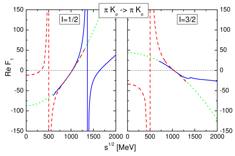
Figure 1: Isospin $\frac{1}{2}$ (left panel) and $\frac{3}{2}$ (right panel) forward scattering amplitude, $F_{1}(q,q;w)=F_{1}(\sqrt{s})$ (see (4)), describing the $\pi\,K_{\mu}$ scattering process in the ’heavy’ SU(3) limit. Sharp vector meson masses are used. The panels show three lines, the line extending to the right (left) shows the s-channel (u-channel) unitarized scattering amplitude. The dotted lines represent the amplitude evaluated at tree-level.

We present out results on s-wave scattering of Goldstone bosons off vector mesons using the leading order chiral SU(3) Lagrangian. Meson resonances with quantum number (I,S) and $J^{P}\!=\!1^{+}$ manifest themselves as poles in the corresponding scattering amplitudes $T^{(I,S)}_{\mu\nu}(\bar{q},q;w)$. We will suppress the index $J^{P}$ in the following studying exclusively the $J^{P}\!=\!1^{+}$ sector. The scattering amplitude takes the form

$$T^{(I,S)}_{\mu\nu}(\bar{q},q;w)=\sum_{ab}\,{\mathcal{Y}}_{ab,\mu\nu}(\bar{q},q;w)\,M^{(I,S)}_{ab}(\sqrt{s}\,)+\cdots\,,$$

$$M^{(I,S)}(\sqrt{s}\,)=\Big{[}1-V^{(I,S)}(\sqrt{s}\,)\,J^{(I,S)}(\sqrt{s}\,)\Big{]}^{-1}\,V^{(I,S)}(\sqrt{s}\,)\,,$$ (20)

where we suppressed further contribution to the scattering amplitude $T^{(I,S)}_{\mu\nu}$ that are off-shell or not of s-wave type. The required projectors in (20) follow from (82) with $J=1$,

$${\mathcal{Y}}_{11,\mu\nu}=\frac{3}{2}\,\frac{w_{\mu}\,w_{\nu}}{w^{2}}-\frac{3}{2}\,g_{\mu\nu}\,,\quad{\mathcal{Y}}_{12,\mu\nu}=-\frac{3}{\sqrt{2}}\,\Big{(}q_{\mu}-\frac{q\cdot w}{w^{2}}\,w_{\mu}\Big{)}\,\frac{w_{\nu}}{\sqrt{w^{2}}}$$

$${\mathcal{Y}}_{22,\mu\nu}=3\,\Big{(}\frac{(\bar{q}\cdot w)\,(w\cdot q)}{w^{2}}-(\bar{q}\cdot q)\Big{)}\,\frac{w_{\mu}\,w_{\nu}}{w^{2}}\,,\qquad$$

$${\mathcal{Y}}_{21,\mu\nu}=-\frac{3}{\sqrt{2}}\,\frac{w_{\mu}}{\sqrt{w^{2}}}\,\Big{(}\bar{q}_{\nu}-\frac{\bar{q}\cdot w}{w^{2}}\,w_{\nu}\Big{)}\,.$$ (21)

The invariant scattering amplitudes are determined by the effective interaction kernel $V^{(I,S)}(\sqrt{s}\,)$ and the loop functions $J^{(I,S)}(\sqrt{s}\,)$. In the $S=2$ sector which involves only a single channel, $K\,K_{\mu}$, the matrix of loop functions takes the form,

$$J_{ab}^{(I,S)}(\sqrt{s}\,)=\left(\begin{array}[]{cc}\frac{3}{2}+\frac{p_{\rm cm}^{2}}{2\,M^{2}}&\;\;\;\frac{p_{\rm cm}^{2}\,\sqrt{M^{2}+p_{\rm cm}^{2}}}{\sqrt{2}\,M^{2}}\\ \frac{p_{\rm cm}^{2}\,\sqrt{M^{2}+p_{\rm cm}^{2}}}{\sqrt{2}\,M^{2}}&\frac{p_{\rm cm}^{4}}{M^{2}}\end{array}\right)_{ab}\!\Big{(}I(\sqrt{s}\,)-I(\mu(I,S))\Big{)}\,,$$ (24)

with $M=M_{K(892)}$ and $m=m_{K(494)}$. In the general case the matrix of loop functions acquires additional dimensions reflecting the presence of inelastic channels. The scalar loop function $I(\sqrt{s}\,)$ was given in (15). For the optimal subtraction scales $\mu(I,S)$ we obtained,

$$\mu(I,0)=M_{\rho(770)}\,,\qquad\mu(I,\pm 1)=M_{K(892)}\,,\qquad\mu(I,\pm 2)=M_{\rho(770)}\,.$$ (25)

It remains to provide explicit expressions for the effective interaction kernel $V^{(I,S)}(\sqrt{s}\,)$. The leading-order chiral SU(3) Lagrangian (1) implies

$$V_{11}^{(I,S)}(\sqrt{s}\,) = \frac{C^{(I,S)}_{WT}}{12\,f^{2}}\,\Big{(}3\,s-M^{2}-\bar{M}^{2}-m^{2}-\bar{m}^{2}-\frac{M^{2}-m^{2}}{s}\,(\bar{M}^{2}-\bar{m}^{2})\Big{)}\,,$$

$$V_{22}^{(I,S)}(\sqrt{s}\,) = -\frac{C^{(I,S)}_{WT}}{12\,f^{2}}\,,\qquad V_{12}^{(I,S)}(\sqrt{s}\,)=V_{21}^{(I,S)}(\sqrt{s}\,)=0\,,$$ (26)

where $(m,M)$ and $(\bar{m},\bar{M})$ are the masses of initial and final mesons. The matrix of coefficients $C^{(I,S)}_{WT}$ is given in Tab. 2. It should be pointed out that though the leading order form of $V_{11}^{(1,+)}$ is determined by the Weinberg-Tomozawa interaction term that this is not the case for $V_{22}^{(1,+)}$. Therefore it is legitimate to use $V_{22}^{(1,+)}=0$ here.

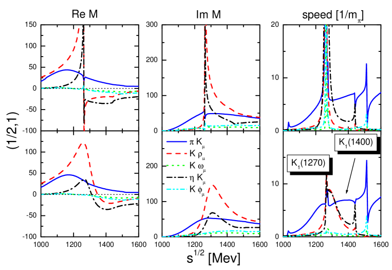
Figure 2: Scattering amplitudes and speeds for meson resonances with $J^{P}\!=\!1^{+}$ and $(I,S)=(\frac{1}{2},1)$ (see (27)). Parameter-free results are obtained in terms of physical masses and $f=90$ MeV. The second row shows the effect of using realistic spectral distributions for the $\rho_{\mu}$- and $K_{\mu}$-mesons.

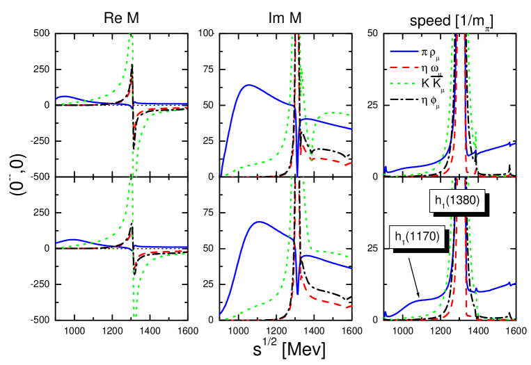
Figure 3: Scattering amplitudes and speeds for meson resonances with $J^{P}\!=\!1^{+}$ and $(I^{G},S)=(0^{-},0)$ (see (27)). Parameter-free results are obtained in terms of physical masses and $f=90$ MeV. The second row shows the effect of using realistic spectral distributions for the $\rho_{\mu}$- and $K_{\mu}$-mesons.

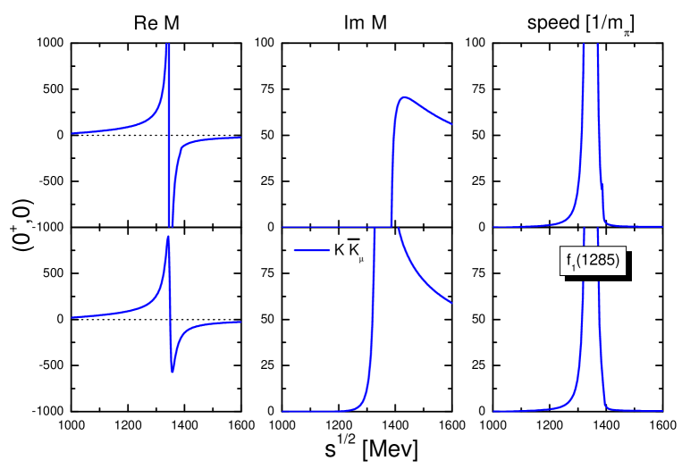
Figure 4: Scattering amplitudes and speeds for meson resonances with $J^{P}\!=\!1^{+}$ and $(I^{G},S)=(0^{+},0)$ (see (27)). Parameter-free results are obtained in terms of physical masses and $f=90$ MeV. The second row shows the effect of using realistic spectral distributions for the $\rho_{\mu}$- and $K_{\mu}$-mesons.

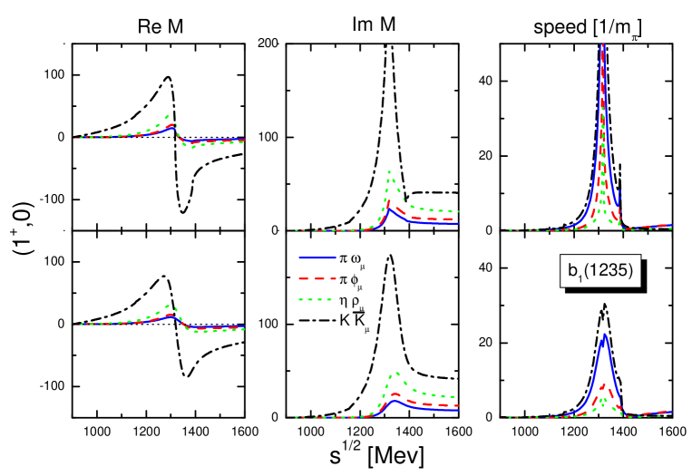
Figure 5: Scattering amplitudes and speeds for meson resonances with $J^{P}\!=\!1^{+}$ and $(I^{G},S)=(1^{+},0)$ (see (27)). Parameter-free results are obtained in terms of physical masses and $f=90$ MeV. The second row shows the effect of using realistic spectral distributions for the $\rho_{\mu}$- and $K_{\mu}$-mesons.

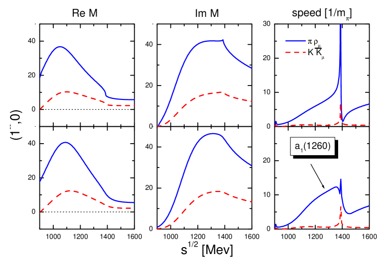
Figure 6: Scattering amplitudes and speeds for meson resonances with $J^{P}\!=\!1^{+}$ and $(I^{G},S)=(1^{-},0)$ (see (27)). Parameter-free results are obtained in terms of physical masses and $f=90$ MeV. The second row shows the effect of using realistic spectral distributions for the $\rho_{\mu}$- and $K_{\mu}$-mesons.

In order to study the formation of meson resonances we generate speed plots as suggested by Höhler [34]. The speed ${\rm Speed}_{ab}^{(I,S)}(\sqrt{s})$ of a given channel $a\,b$, is related to the delay time [35] of a resonance produced in a scattering experiment. It is introduced by [34, 35],

$$t^{(I,S)}_{ab}(\sqrt{s}\,)=\frac{1}{8\,\pi\,\sqrt{s}}\,\Big{(}p^{(a)}_{cm}\,N_{a}^{(I,S)}(\sqrt{s}\,)\,p_{cm}^{(b)}\,N_{b}^{(I,S)}(\sqrt{s}\,)\Big{)}^{1/2}\,M_{ab}^{(I,S)}(\sqrt{s}\,)\,,$$

$${\rm Speed}_{ab}^{(I,S)}(\sqrt{s}\,)=\Big{|}\sum_{c}\,\Big{[}\frac{d}{d\,\sqrt{s}}\,t_{ac}^{(I,S)}(\sqrt{s}\,)\Big{]}\,\Big{(}\delta_{cb}+2\,i\,t_{cb}^{(I,S)}(\sqrt{s}\,)\Big{)}^{*}\Big{|}\,.$$ (27)

The merit of producing speed plot lies in a convenient property of the latter allowing a straight forward extraction of resonance parameters. Assume that a coupled-channel amplitude $M_{ab}(\sqrt{s}\,)$ develops a pole of mass $m_{R}$, with

$$M_{ab}(\sqrt{s}\,)=-\frac{g^{*}_{a}\,g^{\phantom{*}}_{b}\,m_{R}}{\sqrt{s}-m_{R}+i\,\Gamma/2}\,,\qquad\Gamma_{a}=\frac{|g_{a}|^{2}}{4\,\pi}\,|p^{(a)}_{cm}|\,N_{a}(m_{R})\,,$$ (28)

where the total resonance width, $\Gamma$, is given by the sum of all partial widths. For notational simplicity we introduce the parameters, $\Gamma_{a}$, also for channels that are closed, i.e. where the relative momentum $p_{cm}^{(a)}$ in (28) is imaginary. The speed plots take a maximum at the resonance mass $\sqrt{s}=m_{R}$. Some algebra leads to the result

$${\rm Speed}_{aa}(m_{R}\,)=\Bigg{\{}\begin{array}[]{ll}2\,\frac{\Gamma_{a}}{\Gamma^{2}}\,\Big{|}2\,\sum_{c}\,\frac{\Gamma_{c}}{\Gamma}-1\Big{|}\,\qquad\qquad\,{\rm if}\;a={\rm open}\\ 2\,\frac{\Gamma_{a}}{\Gamma^{2}}\,\Big{|}2\,\sum_{c}\,\frac{\Gamma_{c}}{\Gamma}-i\,\Big{|}\,\qquad\qquad\,{\rm if}\;a={\rm closed}\,,\end{array}$$ (31)

$$\Gamma=\sum_{a={\rm open}}\Gamma_{a}\,,$$ (32)

where the summation index $c$ in (32) corresponds to the one in (27). The result (32) clearly demonstrates that the speed [35] of a resonance in a given open channel $a$ is not only a function of the total width parameter $\Gamma$ and the partial width $\Gamma_{a}$. It does depend also on how strongly closed channels couple to that resonance. This is in contrast to the delay time [35] of a resonance for which closed channels do not contribute.

A complementary analysis may be performed by searching for complex poles of the scattering amplitudes on 2nd Riemann sheets. At the leading order level there is however not much point performing such a study. The inclusion of chiral correction terms is expected to be more important than the slightly different values obtained for the resonances masses extracted from speed plots versus from the position of complex poles. To guarantee good analytic properties of the scattering amplitudes it is sufficient to check to what extent the scattering amplitudes satisfy subtracted dispersion-integral representations. An unphysical singularity within the applicability domain would invalidate such a representation. The absence of unphysical structures is also excluded to a large extent by the form of real and imaginary parts of the amplitudes. The resonance like behaviour of all amplitudes is a strong indication that there are no spurious singularities that are relevant, i.e. in the applicability domain.

To explore the multiplet structure of the resonance states we study first the ’heavy’ SU(3) limit [4, 5] with $m_{\pi,K,\eta}\simeq 500$ MeV and $m_{\rho,\omega,K^{*},\phi}\simeq 900$ MeV. In this case all resonance states turn into bound states forming two degenerate octets and one singlet of the SU(3) flavor group with masses 1367 MeV and 1289 MeV respectively. The latter numbers are quite insensitive to the precise value of the subtraction scale. For instance increasing (decreasing) the subtraction scale by 20 $\%$ away from its natural value the octet bound-state mass comes at 1383 MeV (1353 MeV). Our result is a direct reflection of the Weinberg-Tomozawa interaction,

$$8\otimes 8=1\oplus 8\oplus 8\oplus 10\oplus\overline{10}\oplus 27\,,$$ (33)

which predicts attraction in the two octet and the singlet channel. This finding is analogous to the results of [4, 10] that found two degenerate octet and one singlet state in the SU(3) limit of meson-baryon scattering with $J^{P}\!=\!\frac{1}{2}^{-}$. Taking the ’light’ SU(3) limit [5] with $m_{\pi,K,\eta}\simeq 140$ MeV and $m_{\rho,\omega,K^{*},\phi}\simeq 700$ MeV we do not observe any bound-state nor resonance signals anymore. A further interesting limit to study is $N_{c}\to\infty$. Since the scattering kernel is proportional to the $f^{-2}\sim N_{c}^{-1}$ the interaction strength vanishes in that limit and no resonances are generated.

In Fig. 1 we demonstrate the quality of the proposed matching procedure as applied for the forward scattering amplitudes describing the $\pi\,K_{\mu}$ scattering process in the ’heavy’ SU(3) limit. It is shown the term in front of the $g_{\mu\nu}$ structure of the scattering amplitude $T_{\mu\nu}$ as a function of $\sqrt{s}$, where all but the s-wave contributions are evaluated at tree-level for simplicity. The figure clearly illustrates the smooth matching of s-channel and u-channel iterated amplitudes at subthreshold energies. Modifying the subtraction scale by about $10\%$ in either direction does not deteriorate the quality of the matching. It should be pointed out that once chiral correction terms are included in the calculation the quality of the matching is expected to further improve.

Figs. 2-6 show the resonance spectrum that arises using physical masses (first row) and using realistic spectral distributions for the broad vector mesons (second row). Clear signals in the speed plots of the $({\textstyle{1\over 2}},\pm 1)$, $(0^{\pm},0)$ and $(1^{\pm},0)$ channels are seen. No resonance is found in the remaining channels. The resonances can be unambiguously identified with the axial-vector meson resonances ($h_{1}(1170),h_{1}(1380),f_{1}(1285),a_{1}(1260),b_{1}(1235),K_{1}(1270),K_{1}(1400)$).

In the ’heavy’ SU(3) limit the $({\textstyle{1\over 2}},\pm 1)$ channel shows two bound states reflecting the presence of two degenerate octet states. Using physical masses the degeneracy is lifted as illustrated in Fig. 2 and a narrow state at 1263 MeV and a broad state at about 1300 MeV arise. The resonance masses are determined from the maxima of the speed where one has to discard the narrow structures induced by the square root singularities at the various thresholds. Thus, if a resonance is close to a threshold it is difficult to read off its properties from the speed plots. The simple results (28,32) can not be applied. The effect of using realistic spectral distributions for the intermediate $\rho_{\mu}$- and $K_{\mu}$-mesons is demonstrated in the second row of Fig. 2, the first row showing results with sharp vector meson masses. The resonance signal in the speed plots becomes much clearer since using spectral distributions for the broad intermediate states smears away the square-root singularities in the speeds at the corresponding thresholds. In this case we introduce the speed (27) with respect to the invariant amplitudes $M(\sqrt{s}\,)$ evaluated in terms of loop functions folded with spectral distributions of the intermediate states, but use $p_{cm}^{(a)}$ and $p_{cm}^{(b)}$ in (27) defined with respect to sharp masses. Thus the parameters $\Gamma_{a}$ introduced in (28) characterizing the maximum of the speed (32) determine the coupling constants $g_{a}$ via (28) and not the partial-decay width in a channel $a$ where broad intermediate states are used. In contrast, the parameter $\Gamma$ has the interpretation of the total width, i.e. $\Gamma\neq\sum_{a={\rm open}}\Gamma_{a}$ in this case. Our result is quite consistent with the empirical properties of the $K_{1}(1270)$ meson. It has a width of about 90 MeV and decays dominantly into the $K\,\rho_{\mu}-$channel [36]. The second much broader state is assigned a width of about 175 MeV resulting almost exclusively from its decay into the $\pi\,K_{\mu}-$channel [36].

Similarly, in the heavy SU(3) limit the $(0^{-},0)$ channel shows two bound states associated with a singlet and an octet state. Using physical masses a broad state at about 1100 MeV and a narrow state at 1303 MeV should be identified with the $h_{1}(1170)$ and $h_{1}(1380)$ resonance (see Fig. 3). Here we assign the $h_{1}(1380)$-resonance, for which its quantum numbers except its parity and angular momentum $J^{P}=1^{+}$ are unknown, the isospin and G-parity quantum numbers $I^{G}=0^{-}$. This is a clear prediction of the chiral coupled-channel dynamics. The latter state has so far been seen only through its decay into the $K\,\bar{K}_{\mu}$- and $\bar{K}\,K_{\mu}-$channels [37]. Its small width of about 80 MeV [37] is consistent with the narrow structure seen in Fig. 3. The second resonances state in Fig. 3 is most clearly seen in the $\pi\rho_{\mu}-$channel. This is consistent with the empirical properties of the $h_{1}(1170)$ resonance which so far has been seen only through its $\pi\rho_{\mu}-$decay leading to a large width of about 360 MeV [36].

The $(0^{+},0)$-speed (see Fig. 4) shows a bound-state at mass 1341 MeV a value somewhat above the mass of the $f_{1}(1285)$ resonance. Using a spectral distribution for the $K_{\mu}(892)$ in the intermediate states $K\,\bar{K}_{\mu}$ and $\bar{K}\,K_{\mu}$ states a narrow resonance appears. Its width of about 10 MeV is a factor two smaller than the empirical value [36]. The $(1^{+},0)$-speed of Fig. 5 shows a resonance at 1310 MeV to be identified with the $b_{1}(1235)$ resonance. From the maximum of the imaginary part of the scattering amplitudes at the resonance peak one can directly read off ratios of coupling constants. Fig. 5 clearly demonstrates that the smallest coupling constant is predicted for the $\pi\,\omega_{\mu}-$channel. Nevertheless, the hadronic decay of the $b_{1}(1235)$ is completely dominated by the $\pi\,\omega_{\mu}-$channel. This is a simple consequence of phase-space kinematics. The widths of the resonance as indicated by Fig. 5 is quite compatible with the empirical value of about 140 MeV [36]. The $a_{1}(1260)$ resonance is found in the $(1^{-},0)$-speed of Fig. 3 as a broad peak with a mass of about 1300 MeV. Empirically its width is estimated to be about 250-600 MeV [36] resulting from its decay into the $\pi\,\rho-$channel.

The structure of the $h_{1}(1380),f_{1}(1285)$ and $b_{1}(1235)$ resonances as predicted by chiral coupled-channel dynamics is quite intriguing since those resonances couple dominantly to the $K\,\bar{K}_{\mu}-$channel. This implies that the latter channel is the driving force that generates these resonances dynamically. This finding is very much analogous to the structure of the scalar $f_{0}(980)$ resonance that strongly couples to the $K\bar{K}-$channel and emphasizes the importance of the chiral SU(3) symmetry even for non-strange resonances. It should be emphasized that the results obtained here at leading order can be improved further by incorporating chiral correction terms into the analysis. In view of the remarkable success of the leading order Weinberg-Tomozawa interaction one would expect a rapidly converging expansion.

We conclude with an interesting by-product of our analysis. The s-wave scattering lengths of pions with vector mesons are predicted. The scattering length of a pseudo-scalar meson (P) of mass $m$ off a vector meson (V) off mass $M$ is identified,

$$4\,\pi\Big{(}1+\frac{m}{M}\Big{)}\,a^{(I,S)}_{PV}=\frac{3}{4\,M}\,M^{(I,S)}(m+M)\,.$$ (34)

At leading order with $M^{(I,S)}(\sqrt{s}\,)\to V^{(I,S)}(\sqrt{s}\,)$ we recover the Weinberg-Tomozawa theorem,

$$4\,\pi\Big{(}1+\frac{m}{M}\Big{)}\,a^{(I,S)}_{PV}=\frac{m}{2\,f^{2}}\,C^{(I,S)}+{\mathcal{O}}\left(m^{2}\right)\,,$$

$$a_{\pi\,\rho_{\mu}}=\frac{1}{9}\,\Big{(}a^{(0,0)}_{\pi\rho_{\mu}}+3\,a^{(1,0)}_{\pi\,\rho_{\mu}}+5\,a^{(2,0)}_{\pi\,\rho_{\mu}}\Big{)}=0\,,\qquad a_{\pi\,\omega_{\mu}}=\frac{1}{3}\,a^{(1^{+},0)}_{\pi\,\omega_{\mu}}=0\,,$$

$$a_{\pi\,\phi_{\mu}}=\frac{1}{3}\,a^{(1^{+},0)}_{\pi\,\phi_{\mu}}=0\,,\qquad a_{\pi K_{\mu}}=\frac{1}{3}\,\Big{(}a^{(\frac{1}{2},\pm 1)}_{\pi\,K_{\mu}}+2\,a^{(\frac{3}{2},\pm 1)}_{\pi\,K_{\mu}}\Big{)}=0\,,$$ (35)

[fm]	$a^{(0,0)}_{\pi\rho_{\mu}}$	$a^{(1,0)}_{\pi\,\rho_{\mu}}$	$a^{(2,0)}_{\pi\,\rho_{\mu}}$	$a^{(\frac{1}{2},\pm 1)}_{\pi K_{\mu}}$	$a^{(\frac{3}{2},\pm 1)}_{\pi K_{\mu}}$	$a_{\pi\rho_{\mu}}$	$a_{\pi\omega_{\mu}}$	$a_{\pi\phi_{\mu}}$	$a_{\pi K_{\mu}}$
WT	0.45	0.23	-0.23	0.23	-0.12	0	0	0	0
$\chi-BS(3)$	0.69	0.27	-0.20	0.29	-0.10	0.06	0.00	0.01	0.09

Table 3: S-wave scattering length $a_{\pi V}$ with $V=(\rho_{\mu},\omega_{\mu},\phi_{\mu},K_{\mu})$. The first row gives the leading order prediction of Weinberg and Tomozawa (see (35)). These results are confronted in the second row with the scattering length as evaluated in the $\chi-BS(3)$-scheme. Here we use sharp vector meson masses.

which predicts that all isospin averaged scattering lengths of a pion off any vector meson vanish at leading order. In Tab. 3 the scattering lengths as predicted by Weinberg and Tomozawa are confronted with the values obtained form the chiral coupled-channel theory. The deviations obtained are significant in the $(0,0)$ and $(\frac{1}{2},\pm 1)$ channels leading to non-zero and attractive isospin averaged scattering length for the $\rho_{\mu}-$ and $K_{\mu}-$mesons. In the table we present the scattering length obtained for sharp vector-meson masses. In the more realistic case of broad states the scattering lengths are not defined anymore unambiguously. If we use (34) as a definition with sharp values for the mass parameter $M$ but using the amplitudes $M^{(I,S)}(\sqrt{s})$ evaluated in terms of broad intermediate states, the numbers in Tab. 3 change somewhat. In particular the isospin averaged $\pi\rho-$scattering length is reduced to 0.02 fm.

Acknowledgments

M.F.M.L. acknowledges stimulating discussions with M.A. Nowak.

4 Appendix

In this appendix we construct the projectors, ${\mathcal{Y}}^{(JP)}_{ab}(\bar{q},q;w)$, introduced in (6). The latter define the important notion of ’on-shell’ irreducibility. Consider the on-shell scattering amplitude of a pseudo-scalar meson $P(q)$ off a vector meson $V(p,\lambda)$ with polarization $\lambda$,

$$\langle P(\bar{q})\,V(\bar{p},\bar{\lambda})|\,T\,|P(q)\,V(p,\lambda)\rangle$$

$$\qquad=(2\pi)^{4}\,\delta^{4}(q+p-\bar{q}-\bar{p})\,\epsilon^{\dagger}_{\mu}(\bar{p},\bar{\lambda})\,T^{\mu\nu}(\bar{q},q;w)\,\epsilon_{\nu}(p,\lambda)\,,$$ (36)

where we suppress isospin and strangeness quantum numbers for simplicity. The scattering amplitude is subject to various constraints. Covariance together with parity and time reversal conservation lead to a representation of $T_{\mu\nu}(\bar{q},q;w)$ in terms of five scalar amplitudes $F_{i=1,..,5}$, and a complete set of Lorentz tensors $L_{i}^{\mu\nu}$,

$$T^{\mu\nu}(\bar{q},q;w)=\sum_{i=1}^{5}\,F_{i}(\bar{q},q;w)\,L^{\mu\nu}_{i}(\bar{q},q;w)$$ (37)

$$L_{1}^{\mu\nu}=g^{\mu\nu}-\frac{w^{\mu}\,w^{\nu}}{w^{2}}\,,\quad L_{2}^{\mu\nu}=\frac{w^{\mu}\,w^{\nu}}{w^{2}}\,,\quad L_{3}^{\mu\nu}=\frac{w^{\mu}}{\sqrt{w^{2}}}\,\Big{(}\bar{q}^{\nu}-\frac{\bar{q}\cdot w}{w^{2}}\,w^{\nu}\Big{)}\,,\qquad$$

$$L_{4}^{\mu\nu}=\Big{(}q^{\mu}-\frac{q\cdot w}{w^{2}}\,w^{\mu}\Big{)}\,\frac{w^{\nu}}{\sqrt{w^{2}}}\,,\!\!\quad L^{\mu\nu}_{5}=\Big{(}q^{\mu}-\frac{q\cdot w}{w^{2}}\,w^{\nu}\Big{)}\,\Big{(}\bar{q}^{\nu}-\frac{\bar{q}\cdot w}{w^{2}}\,w^{\nu}\Big{)}\,.$$

A further important constraint follows from the two-particle unitarity condition which is efficiently implemented in terms of helicity states [38]. In the center of mass frame with $w_{\mu}=(\sqrt{s},\vec{0})$, helicity matrix elements of the scattering amplitude are decomposed into partial wave amplitudes, $\langle\bar{\lambda}|T^{(J)}|\lambda\rangle$, of given total angular momentum $J$,

$$\epsilon^{\dagger}_{\mu}(\bar{p},\bar{\lambda})\,T^{\mu\nu}(\bar{q},q;w)\,\epsilon_{\nu}(p,\lambda)=\sum_{J}\,(2\,J+1)\,\langle\bar{\lambda}|T^{(J)}|\lambda\rangle\,d^{(J)}_{\lambda\bar{\lambda}}(\theta)$$

$$\epsilon_{\mu}(p)=\left(\begin{array}[]{c}0\\ \frac{\mp 1}{\sqrt{2}}\\ \frac{-i}{\sqrt{2}}\\ 0\end{array}\right)\,,\left(\begin{array}[]{c}\frac{p_{\rm cm}}{M}\\ 0\\ 0\\ \frac{\omega}{M}\end{array}\right)\,,\quad\epsilon_{\mu}(\bar{p})=\left(\begin{array}[]{c}0\\ \frac{\mp\cos\theta}{\sqrt{2}}\\ \frac{-i}{\sqrt{2}}\\ \frac{\pm\sin\theta}{\sqrt{2}}\end{array}\right)\,,\left(\begin{array}[]{c}\frac{p_{\rm cm}}{M}\\ \frac{\omega}{M}\,\sin\theta\\ 0\\ \frac{\omega}{M}\,\cos\theta\end{array}\right)\,,$$ (54)

with $\epsilon_{\mu}(p)=\epsilon_{\mu}(p,\pm 1),\epsilon_{\mu}(p,0)$, $\epsilon_{\mu}(\bar{p})=\epsilon_{\mu}(\bar{p},\pm 1),\epsilon_{\mu}(\bar{p},0)$ and the scattering angle $\theta$. The objects $d^{(J)}_{\lambda\lambda}(\theta)$ are Wigner’s rotation functions and $\omega=(M^{2}+p_{\rm cm}^{2})^{1/2}$. The unitarity constraint now takes the simple form

$$t_{\bar{\lambda}\lambda}^{(J)}=\langle\bar{\lambda}|T^{(J)}|\lambda\rangle\,,\qquad{\rm Im\,}(t^{(J)})^{-1}_{\bar{\lambda}\lambda}=\frac{p_{\rm cm}}{8\pi\,\sqrt{s}}\,\delta_{\bar{\lambda}\lambda}\,.$$ (55)

For the case at hand the channels $J^{P=+}$ and $J^{P=-}$ lead to two-dimensional and one-dimensional projectors respectively. In principal the form of the projectors follows from a boost of the representation (54). However, it is not straight forward to boost partial wave amplitudes. In general this task can be quite tedious. Naive prescriptions typically lead to kinematical singularities and must therefore be rejected. The precise form of the projectors will be derived in the following. In a first step the invariant amplitudes $F_{i}$ are expressed in term of helicity matrix elements, $\phi_{i}$, of the scattering amplitude,

$$\phi_{1}=\epsilon^{\dagger}_{\mu}(\bar{p},+1)\,T^{\mu\nu}(\bar{q},q;w)\,\epsilon_{\nu}(p,+1)+\epsilon^{\dagger}_{\mu}(\bar{p},+1)\,T^{\mu\nu}(\bar{q},q;w)\,\epsilon_{\nu}(p,-1)\,,$$

$$\phi_{2}=\epsilon^{\dagger}_{\mu}(\bar{p},+1)\,T^{\mu\nu}(\bar{q},q;w)\,\epsilon_{\nu}(p,+1)-\epsilon^{\dagger}_{\mu}(\bar{p},+1)\,T^{\mu\nu}(\bar{q},q;w)\,\epsilon_{\nu}(p,-1)\,,$$

$$\phi_{3}=\frac{1}{\sin\theta}\,\epsilon^{\dagger}_{\mu}(\bar{p},0)\,T^{\mu\nu}(\bar{q},q;w)\,\epsilon_{\nu}(p,+1)\,,$$

$$\phi_{4}=\frac{1}{\sin\theta}\,\epsilon^{\dagger}_{\mu}(\bar{p},+1)\,T^{\mu\nu}(\bar{q},q;w)\,\epsilon_{\nu}(p,0)\,,$$

$$\phi_{5}=\epsilon^{\dagger}_{\mu}(\bar{p},0)\,T^{\mu\nu}(\bar{q},q;w)\,\epsilon_{\nu}(p,0)\,.$$ (56)

The five invariant amplitudes can be expressed in terms of the helicity amplitudes $\phi_{i}$,

$$\left(\begin{array}[]{c}F_{1}\\ F_{2}\\ F_{3}\\ F_{4}\\ F_{5}\end{array}\right)=\left(\begin{array}[]{ccccc}-1&0&0&0&0\\ \frac{\omega\,\bar{\omega}\,x}{p_{\rm cm}\,\bar{p}_{\rm cm}\,(1-x^{2})}&-\frac{\omega\,\bar{\omega}\,x^{2}}{p_{\rm cm}\,\bar{p}_{\rm cm}\,(1-x^{2})}&\frac{\sqrt{2}\,\omega\,\bar{M}\,x}{p_{\rm cm}\,\bar{p}_{\rm cm}}&-\frac{\sqrt{2}\,\bar{\omega}\,M\,x}{p_{\rm cm}\,\bar{p}_{\rm cm}}&\frac{M\,\bar{M}}{p_{\rm cm}\,\bar{p}_{\rm cm}}\\ \frac{\bar{\omega}}{\bar{p}_{\rm cm}^{2}\,(1-x^{2})}&-\frac{\bar{\omega}\,x}{\bar{p}_{\rm cm}^{2}\,(1-x^{2})}&\frac{\sqrt{2}\,\bar{M}}{\bar{p}_{\rm cm}^{2}}&0&0\\ \frac{\omega}{p_{\rm cm}^{2}\,(1-x^{2})}&-\frac{\omega\,x}{p_{\rm cm}^{2}\,(1-x^{2})}&0&-\frac{\sqrt{2}\,M}{p_{\rm cm}^{2}}&0\\ \frac{x}{p_{\rm cm}\,\bar{p}_{\rm cm}\,(1-x^{2})}&\frac{-1}{p_{\rm cm}\,\bar{p}_{\rm cm}\,(1-x^{2})}&0&0&0\end{array}\right)\left(\begin{array}[]{c}\phi_{1}\\ \phi_{2}\\ \phi_{3}\\ \phi_{4}\\ \phi_{5}\end{array}\right)\,,$$ (72)

(73)

where we discriminated the masses and relative momenta of the initial and final states with $M,\bar{M}$ and $p_{\rm cm},p_{\rm cm}^{\prime}$. Furthermore we use $x=\cos\theta$ and $\omega=(M^{2}+p_{\rm cm}^{2})^{1/2}$ and $\bar{\omega}=(\bar{M}^{2}+\bar{p}_{\rm cm}^{2})^{1/2}$. According to the general decomposition (54) the amplitudes $\phi_{i}$ can be expressed in terms of partial wave helicity amplitudes $\langle\bar{\lambda}|T^{(J)}|\lambda\rangle$,

$$\phi_{1}=\sum_{J}\,\frac{2\,J+1}{J\,(J+1)}\,\Bigg{(}\langle 1_{+}|T^{(J)}|1_{+}\rangle\,P_{J}^{\prime}(\cos\theta)$$

$$\qquad\qquad\qquad\qquad-\langle 1_{-}|T^{(J)}|1_{-}\rangle\big{(}\cos\theta\,P_{J}^{\prime}(\cos\theta)-J\,(J+1)\,P_{J}(\cos\theta)\Big{)}\Bigg{)}\,,$$

$$\phi_{2}=\sum_{J}\,\,\frac{2\,J+1}{J\,(J+1)}\,\Bigg{(}\langle 1_{-}|T^{(J)}|1_{-}\rangle\,P_{J}^{\prime}(\cos\theta)$$

$$\qquad\qquad\qquad\qquad-\langle 1_{+}|T^{(J)}|1_{+}\rangle\,\big{(}\cos\theta\,P_{J}^{\prime}(\cos\theta)-J\,(J+1)\,P_{J}(\cos\theta)\Big{)}\Bigg{)}\,,$$

$$\phi_{3}=-\frac{1}{\sqrt{2}}\,\sum_{J}\,\frac{2\,J+1}{\sqrt{J\,(J+1)}}\,\,\langle 0|T^{(J)}|1_{+}\rangle\,P^{\prime}_{J}(\cos\theta)\,,$$

$$\phi_{4}=+\frac{1}{\sqrt{2}}\,\sum_{J}\,\frac{2\,J+1}{\sqrt{J\,(J+1)}}\,\langle 1_{+}|T^{(J)}|0\rangle\,P^{\prime}_{J}(\cos\theta)\,,$$

$$\phi_{5}=+\sum_{J}\,(2\,J+1)\,\langle 0|T^{(J)}|0\rangle\,P_{J}(\cos\theta)\,,$$ (74)

where we introduced parity eigenstates with $\langle 1_{\pm},J|=(\pm\langle+1,J|+\langle-1,J|)/\sqrt{2}$ and applied the useful identities [39]

$$d^{(J)}_{00}(\theta)=P_{J}(\cos\theta)\,,\qquad d^{(J)}_{\pm 10}(\theta)=\mp\frac{\sin\theta}{\sqrt{J\,(J+1)}}\,P_{J}^{\prime}(\cos\theta)=-d^{(J)}_{0\pm 1}(\theta)\,,$$

$$d^{(J)}_{\pm 11}(\theta)=\frac{1\pm\cos\theta}{J\,(J+1)}\,\Big{(}P_{J}^{\prime}(\cos\theta)\mp(1\mp\cos\theta)\,P_{J}^{\prime\prime}(\cos\theta)\Big{)}=d^{(J)}_{1\pm 1}(\theta)\,.$$ (75)

It now appears straightforward to construct the projectors, ${\mathcal{Y}}^{(JP_{-})}(\bar{q},q;w)$, associated with $\langle 1_{-}|$ and parity $P_{-}=(-1)^{J}$. It is a single-channel projector. However, it is important to properly boost the results (4,73,74) obtained in the center of mass frame. As was pointed out in [3] it is incorrect to identify always

$$\cos\theta\leftrightarrow\frac{Y_{q\bar{q}}}{\sqrt{Y_{qq}\,Y_{\bar{q}\bar{q}}}}\,,$$ (76)

with

$$Y_{qq}=\frac{(w\cdot q)^{2}}{w^{2}}-q^{2}\,,\qquad Y_{\bar{q}\bar{q}}=\frac{(w\cdot\bar{q})^{2}}{w^{2}}-\bar{q}^{2}\,,\qquad$$

$$Y_{q\bar{q}}=\frac{(w\cdot q)\,(w\cdot\bar{q})}{w^{2}}-q\cdot\bar{q}\,.$$ (77)

It is clear, that if (76) is used for instance in $P_{J}(\cos\theta)$, kinematical singularities at $Y_{qq}=0$ or $Y_{\bar{q}\bar{q}}=0$ arise that are unphysical. The latter are realized at the off-shell surfaces defined by $(p\cdot q)^{2}=p^{2}\,q^{2}$ and $(\bar{p}\cdot\bar{q})^{2}=\bar{p}^{2}\,\bar{q}^{2}$. Therefore the naive prescription (76) must be rejected. It would spoil the analytic properties of the scattering amplitude. In order to proceed it is necessary to boost objects only that posses a proper frame independent representation. For instance this is the case for $(p_{\rm cm}\,p_{\rm cm}^{\prime})^{n}\,P_{n}(\cos\theta)$. We identify

$$(p_{\rm cm}\,p_{\rm cm}^{\prime})^{n}\,P_{n}(\cos\theta)\to\sum_{k=0}^{n}\,c^{(n)}_{k}\,\,Y^{(n-k)/2}_{qq}\,Y^{(n-k)/2}_{\bar{q}\bar{q}}\,Y^{k}_{q\bar{q}}\,,$$

$$P_{n}(x)=\sum_{k=0}^{n}\,c^{(n)}_{k}\,x^{k}\,,\qquad c^{(n)}_{n-2\,r}=(-1)^{r}\,\frac{(2\,n-2\,r)\,!}{2^{n}\,r\,!\,(n-r)\,!\,(n-2\,r)\,!}\,.$$ (78)

Note that the combination $n-k$ in (78) is always even and positive. Thus no square-root singularities are picked up in (78). An analogous replacement is applicable for $(p_{\rm cm}\,p_{\rm cm}^{\prime})^{n}\,x\,P^{\prime}_{n}(x)$. We derive

$${\mathcal{Y}}^{(JP_{-})}_{\mu\nu}(\bar{q},q;w)=\sum_{k=1}^{J}\frac{2\,J+1}{J\,(J+1)}\,c^{(J)}_{k}\,k\,(k-1)\,Y^{(J-k)/2}_{qq}\,Y^{(J-k)/2}_{\bar{q}\bar{q}}\,Y^{k-1}_{q\bar{q}}$$

$$\quad\times\Bigg{(}\Big{(}\frac{1}{k-1}-\frac{J\,(J+1)}{k\,(k-1)}\Big{)}\,Y_{q\bar{q}}\,L_{1,\mu\nu}-\frac{(\bar{q}\cdot w)\,(w\cdot q)}{w^{2}}\,L_{2,\mu\nu}$$

$$\qquad-\frac{w\cdot\bar{q}}{\sqrt{w^{2}}}\,\frac{Y_{qq}}{Y_{q\bar{q}}}\,\,L_{3,\mu\nu}-\frac{w\cdot q}{\sqrt{w^{2}}}\,\frac{Y_{\bar{q}\bar{q}}}{Y_{q\bar{q}}}\,L_{4,\mu\nu}-\frac{k}{k-1}\,L_{5,\mu\nu}\Bigg{)}\,,$$

$$P_{-}=(-1)^{J}\,,$$ (79)

where the coefficients $c_{k}^{(J)}$ are given in (78) and the Lorentz tensors $L_{i,\mu\nu}$ were introduced in (4). The projector is introduced with respect to

$$|1^{(-)}_{c},J\rangle=p_{\rm cm}^{J}\,|1_{-},J\rangle\,,$$ (80)

rather than $|1_{-},J\rangle$. This rescaling provides the necessary phase space factor $(p_{\rm cm}\,\bar{p}_{\rm cm})^{J}$ required for the proper definition of the projector. We emphasize that the projectors ${\mathcal{Y}}^{(JP_{-})}_{\mu\nu}(\bar{q},q;w)$ are regular at the kinematical surfaces defined by $(p\cdot q)^{2}=p^{2}\,q^{2}$ and $(\bar{p}\cdot\bar{q})^{2}=\bar{p}^{2}\,\bar{q}^{2}$. The singularity at $w^{2}=0$ can be avoided by rescaling the projectors by an appropriate power in $\sqrt{w^{2}}$. Since the kinematical point $w^{2}=0$ is far outside the region where we will be using the projectors this is not an issue here.

We continue and derive the projectors for the remaining sector. Here an additional complication arises. If one tries to introduce a projector matrix with respect to the helicity states $(\langle 1_{+},J|,\langle 0,J|)$ it is impossible to arrive at a result that is free of kinematical singularities. A non-unitary transformation is required to new states $(\langle 1^{(+)}_{c},J|,\langle 2^{(+)}_{c},J|)$ with respect to which projectors can be obtained that are free of kinematical singularities,

$$|1^{(+)}_{c},J\rangle=p_{\rm cm}^{J-1}\,\Big{(}|1_{+},J\rangle+\sqrt{\frac{J}{1+J}}\,\frac{\omega}{M}\,|0,J\rangle\Big{)}\,,\;\,|2^{(+)}_{c},J\rangle=\frac{p_{\rm cm}^{J+1}}{M}\,|0,J\rangle\,.$$ (81)

The projector matrix follows

$${\mathcal{Y}}^{(JP_{+})}_{11,\mu\nu}(\bar{q},q;w)=\sum_{k=1}^{J}\frac{2\,J+1}{J\,(J+1)}\,k\,(k-1)\,Y^{(J-k)/2}_{qq}\,Y^{(J-k)/2}_{\bar{q}\bar{q}}\,Y^{k-2}_{q\bar{q}}$$

$$\quad\quad\times\Bigg{(}-\frac{1}{k-1}\,c^{(J)}_{k}\,Y_{\bar{q}q}\,L_{1,\mu\nu}+c^{(J)}_{k}\,L_{5,\mu\nu}$$

$$\quad\qquad+c^{(J-1)}_{k}\,\frac{w\cdot\bar{q}}{\sqrt{w^{2}}}\,\left(\frac{Y_{qq}}{Y_{\bar{q}\bar{q}}}\right)^{1/2}\,L_{3,\mu\nu}+c^{(J-1)}_{k}\,\frac{w\cdot q}{\sqrt{w^{2}}}\,\left(\frac{Y_{\bar{q}\bar{q}}}{Y_{qq}}\right)^{1/2}\,L_{4,\mu\nu}$$

$$\quad\qquad+\frac{k-1-J}{k-1}\,c^{(J-1)}_{k}\,\frac{(\bar{q}\cdot w)\,(w\cdot q)}{w^{2}}\,\frac{Y_{q\bar{q}}}{(Y_{\bar{q}\bar{q}}\,Y_{qq})^{1/2}}\,L_{2,\mu\nu}\Bigg{)}\,,$$

$${\mathcal{Y}}^{(JP_{+})}_{12,\mu\nu}(\bar{q},q;w)=\sum_{k=1}^{J}\frac{2\,J+1}{\sqrt{J\,(J+1)}}\,k\,Y^{(J-k)/2}_{qq}\,Y^{(J-k)/2}_{\bar{q}\bar{q}}\,Y^{k-1}_{q\bar{q}}$$

$$\quad\quad\times\Bigg{(}-c^{(J-1)}_{k}\,\frac{\bar{q}\cdot w}{\sqrt{w^{2}}}\,\left(\frac{Y_{qq}}{Y_{\bar{q}\bar{q}}}\right)^{1/2}\,L_{2,\mu\nu}-c^{(J)}_{k}\,L_{4,\mu\nu}\Bigg{)}\,,$$

$${\mathcal{Y}}^{(JP_{+})}_{21,\mu\nu}(\bar{q},q;w)=\sum_{k=1}^{J}\frac{2\,J+1}{\sqrt{J\,(J+1)}}\,k\,Y^{(J-k)/2}_{qq}\,Y^{(J-k)/2}_{\bar{q}\bar{q}}\,Y^{k-1}_{q\bar{q}}$$

$$\quad\quad\times\Bigg{(}-c^{(J-1)}_{k}\,\frac{w\cdot q}{\sqrt{w^{2}}}\left(\frac{Y_{\bar{q}\bar{q}}}{Y_{qq}}\right)^{1/2}L_{2,\mu\nu}-c^{(J)}_{k}\,L_{3,\mu\nu}\Bigg{)}\,,$$

$${\mathcal{Y}}^{(JP_{+})}_{22,\mu\nu}(\bar{q},q;w)=\sum_{k=0}^{J}\big{(}2\,J+1\big{)}\,Y^{(J-k)/2}_{qq}\,Y^{(J-k)/2}_{\bar{q}\bar{q}}\,Y^{k}_{q\bar{q}}\;c^{(J)}_{k}\,L_{2,\mu\nu}\,,$$

$$P_{+}=(-1)^{J+1}\,,$$ (82)

We observe that the projectors ${\mathcal{Y}}^{(JP_{+})}_{ij,\mu\nu}(\bar{q},q;w)$ are regular at the kinematical surfaces defined by $(p\cdot q)^{2}=p^{2}\,q^{2}$ and $(\bar{p}\cdot\bar{q})^{2}=\bar{p}^{2}\,\bar{q}^{2}$. Moreover we point out that none of the projectors depends on any of the masses of initial or final states. This is an important property of the projector since it implies that the projectors can also be applied also in the case where initial and final particle have a spectral distribution.

In order to complete the definition of on-shell irreducibility it remains to express the invariant amplitude $M^{(JP)}_{ij}(\sqrt{s}\,)$ in terms of the invariant amplitudes $F_{i}(\bar{q},q;w)$. Some algebra leads to,

$$M_{11}^{(JP_{-})}=\int_{-1}^{+1}\frac{dx}{2}\,\frac{1}{(p_{\rm cm}\,\bar{p}_{\rm cm})^{J}}\,\Bigg{(}-P_{J}(x)\,F_{1}-{\textstyle{1-x^{2}\over{J\,(J+1)}}}\,P^{\prime}_{J}(x)\,p_{\rm cm}\,\bar{p}_{\rm cm}\,F_{5}\Bigg{)}\,,$$

$$M_{11}^{(JP_{+})}=\int_{-1}^{+1}\frac{dx}{2}\,\frac{1}{(p_{\rm cm}\,\bar{p}_{\rm cm})^{J-1}}\,\Bigg{(}\Big{(}-{\textstyle{1-x^{2}\over{J\,(J+1)}}}\,P^{\prime}_{J}(x)-x\,\,P_{J}(x)\Big{)}\,F_{1}$$

$$\qquad\qquad\quad\quad+\Big{(}{\textstyle{1-x^{2}\over{J\,(J+1)}}}\,x\,P_{J}^{\prime}(x)-(1-x^{2})\,P_{J}(x)\Big{)}\,p_{\rm cm}\,\bar{p}_{\rm cm}\,F_{5}\Bigg{)}\,,$$

$$M_{12}^{(JP_{+})}=\int_{-1}^{+1}\frac{dx}{2}\,\frac{\bar{p}_{\rm cm}^{2}}{(p_{\rm cm}\,\bar{p}_{\rm cm})^{J+1}}\,\Bigg{(}\sqrt{{\textstyle{J\over{J+1}}}}\,P_{J+1}(x)\,\omega\,F_{1}-{\textstyle{1-x^{2}\over{\sqrt{J\,(J+1)}}}}\,P_{J}^{\prime}(x)\,p_{\rm cm}^{2}\,F_{4}$$

$$\qquad\qquad\quad\quad+\sqrt{{\textstyle{J\over{J+1}}}}\,\Big{(}P_{J}(x)-x\,P_{J+1}(x)\Big{)}\,\omega\,p_{\rm cm}\,\bar{p}_{\rm cm}\,F_{5}\Bigg{)}\,,$$

$$M_{21}^{(JP_{+})}=\int_{-1}^{+1}\frac{dx}{2}\,\frac{p_{\rm cm}^{2}}{(p_{\rm cm}\,\bar{p}_{\rm cm})^{J+1}}\,\Bigg{(}\sqrt{{\textstyle{J\over{J+1}}}}\,P_{J+1}(x)\,\bar{\omega}\,F_{1}-{\textstyle{1-x^{2}\over{\sqrt{J\,(J+1)}}}}\,P_{J}^{\prime}(x)\,\bar{p}_{\rm cm}^{2}\,F_{3}$$

$$\qquad\qquad\quad\quad+\sqrt{{\textstyle{J\over{J+1}}}}\,\Big{(}P_{J}(x)-x\,P_{J+1}(x)\Big{)}\,\bar{\omega}\,p_{\rm cm}\,\bar{p}_{\rm cm}\,F_{5}\Bigg{)}\,,$$

$$M_{22}^{(JP_{+})}=\int_{-1}^{+1}\frac{dx}{2}\,\frac{1}{(p_{\rm cm}\,\bar{p}_{\rm cm})^{1+J}}\,\Bigg{(}-{\textstyle{2\,J+1\over{J+1}}}\,P_{J+1}(x)\,\omega\,\bar{\omega}\,F_{1}$$

$$\qquad\qquad\quad\quad+P_{J}(x)\,p_{\rm cm}\,\bar{p}_{\rm cm}\,F_{2}-P_{J+1}(x)\,\Big{(}\omega\,\bar{p}_{\rm cm}^{2}\,F_{3}+\bar{\omega}\,p_{\rm cm}^{2}\,F_{4}\Big{)}$$

$$\qquad\qquad\quad\quad+\Big{(}{\textstyle{2\,J+1\over{J+1}}}\,x\,P_{J+1}(x)-{\textstyle{J\over{J+1}}}\,P_{J}(x)\Big{)}\,\omega\,\bar{\omega}\,p_{\rm cm}\,\bar{p}_{\rm cm}\,F_{5}\Bigg{)}\,,$$ (83)

where $x=\cos\theta$ and $\omega=(M^{2}+p_{\rm cm}^{2})^{1/2}$ and $\bar{\omega}=(\bar{M}^{2}+\bar{p}_{\rm cm}^{2})^{1/2}$. In (83) the invariant amplitudes $F_{i}(\sqrt{s}\,,x)$ are considered as a function of $\sqrt{s}=\omega+(m^{2}+p_{\rm cm}^{2})^{1/2}=\bar{\omega}+(\bar{m}^{2}+p_{\rm cm}^{2})^{1/2}$ and the scattering angle $\theta$.

The results (79, 82, 83) specify the notion of on-shell irreducibility. For any two-body amplitude the on-shell irreducible part can be evaluated by first seeking a representation in terms of the Lorentz tensors $L_{i,\mu\nu}$. The required coefficient functions in front of the projectors can be evaluated via (83). We emphasize that the concept of on-shell irreducibility smoothly carries over to the case where initial or final states have spectral distributions rather than well defined energy-momentum dispersions. In this case the use of the projector makes sure that two-body unitarity is fulfilled exactly. Though the evaluation of the on-shell irreducible part of the effective interaction $V$ will depend on approximate mass parameters of the initial and final states the latter will not affect the unitarity condition. All ambiguities related to the finite width of initial or final states are moved into the interaction kernel. A particular choice of an approximate mass parameter influences only what is leading order in the kernel and what will be treated as a correction.

References

[1]
M.F.M. Lutz and E. E. Kolomeitsev, Proc. of Int. Workshop XXVIII
on Gross Properties of Nuclei and Nuclear Excitations, Hirschegg,
Austria, January 16-22, 2000.
[2]
M.F.M. Lutz und E.E. Kolomeitsev, Found. Phys. 31 (2001) 1671.
[3] M.F.M. Lutz and E. E. Kolomeitsev, Nucl. Phys. A
700 (2002) 193.
[4]
C. García-Recio, M.F.M. Lutz and J. Nieves, nucl-th/0305100.
[5]
E.E. Kolomeitsev and M.F.M. Lutz, nucl-th/0305101.
[6] J. Nieves and E. Ruiz Arriola, Phys. Rev. D
63, (2001) 076001.
[7] C. García-Recio,
J. Nieves, E. Ruiz Arriola and M. J. Vicente-Vacas, Phys. Rev.
D 67 (2003) 076009.
[8] A. Ramos, E. Oset and C. Bennhold,
Phys. Rev. Lett. 89 (2002) 252001.
[9]
E. Oset, A. Ramos, C. Bennhold, Phys. Lett. B 527 (2002)
99.
[10]
D. Jido et al., nucl-th/0303062.
[11] H.W. Wyld, Phys. Rev. 155 (1967) 1649.
[12] R.H. Dalitz, T.C. Wong and G. Rajasekaran,
Phys. Rev. 153 (1967) 1617.
[13]
J.S. Ball and W.R. Frazer, Phys. Rev. Lett. 7 (1961) 204.