Invariant correlational entropy as a signature of quantum phase transitions in nuclei

Abstract

We study phase transformations in finite nuclei as a function of interaction parameters. The signature of a transition is given by invariant correlational entropy that reflects the sensitivity of an individual many-body state to changes of external parameters; peaks in this quantity indicate the critical regions. This approach is able to reveal the pairing phase transition, identify the isovector and isoscalar pairing regions and determine the role of other interactions. We show the examples of the phase diagram in the parameter space.

Recently, an appreciable effort has been applied to understand and classify quantum phase transitions sachdev99 ; borrmann01 ; mulken01 . Although the concept of a phase transition is strictly applicable in the thermodynamic limit only, there are numerous examples of structural changes in mesoscopic systems, ranging from molecular clusters and semiconductors to atomic nuclei or quark systems, under variation of control parameters. Proper understanding of such transitions is crucial for areas from cosmology and formation of the universe to quantum computing and decoherence. The typical feature of phase transitions in small systems is the absence of discontinuities in the observables, and, therefore, difficulty for identification and classifications of such transitions. The counterparts of phase changes in small systems involve restructuring, critical sensitivity to parameters, and chaotic large-scale fluctuations. In this work we study mesoscopic phase transitions in atomic nuclei using shell model interactions, which are known to reproduce the low-lying states in selected nuclei with a remarkable quality. The instrument we suggest for such studies can be similarly applied to other finite quantum systems.

We identify the presence of a phase transformation as an enhancement in the invariant correlational entropy (ICE) which was introduced in sokolov98 . ICE provides a measure of sensitivity of a given state in the many-body system to variations of external parameters. From earlier studies of bosonic models the increase of ICE is known to be associated with critical points cejnar01 . We do not consider here thermal phase transitions for a system in a heat bath although it is possible, see sokolov98 and cejnar01 , to introduce an effective temperature as a measure of fluctuations in the dynamical response to the change of parameters.

Following sokolov98 , we assume a Hamiltonian $H(\lambda)$ that depends on a parameter $\lambda,$ so that, in an arbitrary basis $|k\rangle,$ any eigenstate $|\alpha(\lambda)\rangle$ of $H(\lambda)$ can be decomposed as $|\alpha(\lambda)\rangle=\sum_{k}C_{k}^{\alpha}(\lambda)|k\rangle\,.$ The ICE is then defined as

$$S^{\alpha}(\lambda)=-\text{Tr}\left\{\rho^{\alpha}\ln(\rho^{\alpha})\right\},$$ (1)

where $\rho^{\alpha}$ is the density matrix of the state $|\alpha\rangle$ in the basis $k$ averaged over a small region ${\lambda}\in[\lambda,\lambda+\delta]$,

$$\rho^{\alpha}_{kk^{\prime}}(\lambda)=\overline{C^{\alpha}_{k}C^{\alpha*}_{k^{\prime}}}.$$ (2)

The discussion of various entropy-like quantities of individual wave functions can be found in Ref. sokolov98 . ICE is basis-independent von Neumann entropy that reflects the correlations between the wave function components along the evolution path determined by the parameter $\lambda$. It should not be confused with basis-dependent Shannon information entropy

$$I^{\alpha}=-\sum_{k}|C^{\alpha}_{k}|^{2}\ln|C^{\alpha}_{k}|^{2}$$ (3)

that was extensively used for studying the degree of complexity of the state $|\alpha\rangle$ with respect to the given basis $|k\rangle$ izrailev90 ; big without taking into account correlations between the amplitudes $C^{\alpha}_{k}$.

For a pure state, i.e. without averaging, the density matrix has a single non-zero eigenvalue equal to one because of the normalization ${\rm Tr}\,\rho=1$. This results in $S^{\alpha}=0.$ After averaging, we deal with a mixed state, and the eigenvalues of $\rho$ deviate from the trivial limit. As shown in sokolov98 , higher orders of perturbation theory bring in new non-zero eigenvalues. Averaging over only two discrete points $\lambda$ and $\lambda^{\prime}$ leads to a factorized matrix $\rho^{\alpha}$ with two non-zero eigenvalues

$$r^{\alpha}_{\pm}=\left(1\pm|\langle\alpha(\lambda)|\alpha(\lambda^{\prime})\rangle|\right)/2.$$ (4)

Now ICE can change from 0 (in the absence of any evolution of the state) to the maximum value $\ln 2$ reached for the orthogonal states in the representative points $\lambda$ and $\lambda^{\prime}$. Thus, ICE in a basis-independent way shows how “quickly” the eigenstate $\alpha$ reorients due to sudden change of interaction from $H(\lambda)$ to $H(\lambda^{\prime}).$ This makes ICE an ideal tool for studying phase transitions.

We apply the ICE tool to spherical shell-model systems, where the general Hamiltonian includes independent particle orbitals and two-body residual interactions,

$$H=\sum_{\bf 1}\epsilon_{1}a^{\dagger}_{\bf 1}a_{\bf 1}+\sum_{{1}{2}{3}{4}L\Lambda}\,V^{({1}{2};{3}{4})}_{L}\,\left(P^{({1}\,{2})}_{L\,\Lambda}\right)^{\dagger}\,P^{({3}\,{4})}_{L\,\Lambda}\,.$$ (5)

Here pair creation and annihilation operators couple corresponding single-particle operators to an appropriate angular momentum, i.e. $P^{(12)}=(1+\delta_{12})^{-1/2}[a_{\bf 1}\times a_{\bf 2}]_{L\Lambda}.$ The usual pairing interaction is given by the $L=0$ term. We suppress the isospin degree of freedom, but it is straightforward to include it in direct analogy to angular momentum.

We start with a simple model, where the pairing interaction is known to result in a phase transition in the BCS approach. $N$ identical nucleons occupy two single-particle orbitals $\epsilon_{1}=-\epsilon$ and $\epsilon_{2}=\epsilon$ of equal spherical degeneracy $\Omega_{1}=\Omega_{2}=\Omega$. They interact via off-diagonal pair transfers determined by a parameter $\lambda$ as $V^{(11;22)}_{0}=V^{(22;11)}_{0}=-2\lambda/\Omega.$ Let the system be half-occupied, $N=\Omega$, which sets the chemical potential $\mu=0.$ It is known from the BCS theory that the pairing interaction causes the normal to superconducting phase transition, and, in the asymptotic limit of a large system, any weak but attractive pairing is sufficient for creating the Cooper instability. For a finite system the BCS solution is approximate. Because of the finite single-particle level spacing at the Fermi surface, the BCS phase transition takes place at the critical strength value,

$$\lambda_{c}^{2}=\frac{16\epsilon^{2}}{\Omega^{2}}.$$ (6)

The exact solution of the problem PRC65 determines the ground state and the excited states of two types, “pair-vibrational” states with seniority $s=0$ and redistribution of the pairs, and states with broken pairs and $s\neq 0$. For each state one can calculate ICE varying $\lambda$. The results for the ground and two lowest pair-vibration states calculated with the averaging interval $\delta=0.01$ are shown in Fig. 1. The clear ICE peak in the ground state indicates the presence of the phase transition. For $\epsilon=1$ and $\Omega=N=16$ the BCS theory predicts a phase transition at $\lambda_{c}=0.25$. Corrections to the BCS vacuum PRC65 ; rabhi02 make $\lambda_{c}$ slightly larger, and ICE reaches its maximum at $\lambda_{c}=0.3.$ In the excited states the phase transition is quenched. The first excited state is collective and exhibits a broadened peak of ICE. For the second excited state the peak disappears although there is still a maximum of $S(\lambda)$ at $\lambda=0$ indicating an enhanced sensitivity to switching on pairing.

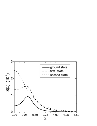
Figure 1: Invariant correlational entropy of the ground and two lowest pair-vibrational excited states calculated for the two-level pairing model as a function of pairing strength $\lambda$ and with averaging interval $\delta=0.01.$

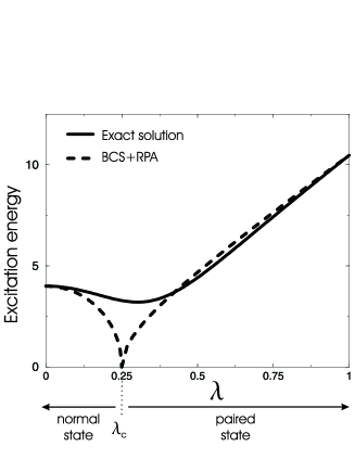
Figure 2: Energy of the first pair-vibration level in the BCS+RPA (dashed line with instability at $\lambda_{c}$) and exact solution (solid line) that shows softening at the shifted point.

It is also possible to recognize the signature of the phase transition in the exact energy spectrum. In Fig. 2 the excitation energy of the first pair vibration state is shown. The softening of this mode at the same point $\lambda_{c}=0.3$ is characteristic for the phase transition and supports the level crossing interpretation. With the dashed line we show the same state in the random phase approximation, RPA, built on the BCS condensate PRC65 . The instability of the BCS+RPA approach for a soft mode is an artifact of the invalid approximation, see also rabhi02 .

Figure 3: ICE (computed with averaging interval $\delta=0.1$), upper panel, and occupancy of the lowest $f_{7/2}$ orbital, lower panel, as a function of pairing strength for different scales of non-pairing interactions, $\lambda_{np}=$0.2, 1, 2, 3, and 4.

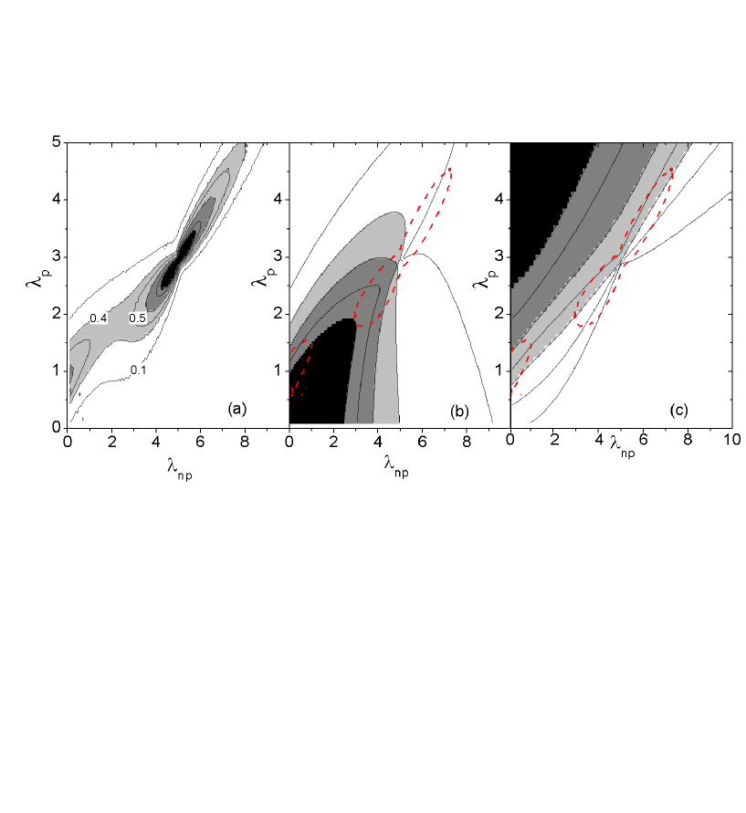
Figure 4: Phase diagram of the shell model ground state wave function of ⁴⁸Ca. The parameters are the pairing strength $\lambda_{p}$ and an overall strength $\lambda_{np}$ of remaining non-pairing matrix elements. Panel (a) shows ICE with the averaging interval $\delta=0.05$ in both scales. ICE is normalized by a factor 0.015. Panels (b) and (c) show the occupancy of the $f_{7/2}$ orbital and the average number of correlated pairs ${\cal N}_{1}$, Eq. (7), respectively. To emphasize the consistency between these quantities and location of phase changes, the dotted contours in panels (b) and (c) outline the region where ICE is enhanced above the value of 0.5.

As a realistic example we consider the case of the $N=28$ subshell closure in ⁴⁸Ca. It has been emphasized in Ref. volyaEP that although the BCS approach predicts no paired ground state in this nucleus, the exact solution indicates presence of pairing correlations. The interplay of weak pairing and self-consistent monopole renormalization of single-particle energies leads to correlation energy of nearly 2 MeV. The specifics of pairing correlations and self-consistent mean field in $N=28$ nuclei have recently been a subject of experimental cottle02 and theoretical werner96 ; lalazissis99 interest. Here we go beyond the mean field and solve exactly the many-body Hamiltonian with the effective interaction richter91 in the plane of parameters $\lambda_{p}$ and $\lambda_{np}$ that scale all pairing ($T=1$, $L=0$) and remaining non-pairing matrix elements, respectively.

The results for the ground state of ⁴⁸Ca are given in Figs. 3 and 4. The peaks in ICE in the upper panel in Fig. 3 unambiguously identify the pairing phase transition. The drop in the occupancy of the lowest $f_{7/2}$ orbital shown in lower panel is also consistent with this behavior indicating the disappearance of subshell closure and a transition into a paired state. Five curves in both panels of Fig. 3 allow one to track the evolution of the phase transition as a function of strength $\lambda_{np}$ of non-pairing matrix elements. Panel (a) in Fig. 4 shows ICE with a contour plot in the $\lambda_{p}$ - $\lambda_{np}$ plane. Higher values are indicated with shaded areas. ICE is enhanced along the diagonal outlining, as in a phase diagram, the boundary between the normal Fermi state (lower right) and superconducting paired state (upper left). The panel (c) confirms this identification of phases. Here the effective number of pairs ${\cal N}_{T=1}$, computed as an expectation value of the operator big

$$\hat{{\cal N}}_{T}=\sum_{12}\left(P^{(11)}_{L=1-T,\,T}\right)^{\dagger}P^{(22)}_{L=1-T,\,T}$$ (7)

in the ground state, is shown. This quantity reaches its maximum value ${\cal N}_{1}=(1/4)(N-s)(\Omega-N-s+2)$, where $\Omega$ is the total capacity of the valence space, and seniority $s$ gives the number of unpaired particles, in the degenerate limit, i.e. when the pairing becomes so strong that differences in single-particle energies can be ignored. The maximum number of pairs is expected for a fully paired state with $s=0$, which for our model, with $\Omega=20$ and $N=8$, leads to ${\cal N}_{1}=28$. The non-pairing interactions create a random background, mixing seniorities and adding some statistical number of pairs to any state. This background can be estimated by averaging operator $\hat{{\cal N}}_{1}$ over all many-body states, $\overline{{\cal N}_{1}}=[N(N-1)]/[2(\Omega-1)]$, which gives $\overline{{\cal N}_{1}}\approx 1.5$ in our model. Indeed, the major part of the valley in Fig. 4(c), shown as a white area, is levelled at around this value. In the phase transition region, along with the enhancement of ICE, the number of correlated pairs quickly rises, finally becoming close to 28. The full saturation at ${\cal N}_{1}=28$ is not expected to be reached, since it is only possible for the constant pairing interaction.

The enhancement of ICE not only allows one to localize the phase transition but also quantifies the sharpness of the transformation and the size of the critical region. In macroscopic BCS theory it is usually assumed that the non-pairing interactions renormalize quasiparticles but essentially do not participate in the phase transition. The shell model analysis big demonstrated that this is not the case, at least in a finite system. As seen from Figs. 3 and 4, the scaling factor $\lambda_{np}$ plays a significant role in the overall picture. At $\lambda_{np}=0$, the pairing phase transition is quite sharp and takes place slightly below $\lambda_{p}=1.0.$ Indeed, the comparison of earlier studies volyaEP ; belyaev shows that pairing would be stable and treatable with the BCS if no other interactions had been present in ⁴⁸Ca. Presence of other parts of residual interaction softens and widens the transitional region, putting the physical state $\lambda_{np}=\lambda_{p}=1$ in the normal domain below the phase transition peak, although within the region of enhanced pair fluctuations. It was also shown earlier big that other interactions destroy the purity of the seniority classes (in the first order the ground state acquires the contribution of $s=4$) moving the dynamics to many-body quantum chaos big ; PRC65 .

The non-pairing interactions shape the properties of the mean field and redefine effective single-particle energies; on the other hand, they induce chaotic residual dynamics. In Fig. 4(b), the occupancy of the $f_{7/2}$ orbital is mapped in the same parameter space. The lowest $f_{7/2}$ level in ⁴⁸Ca is separated from other single-particle levels by almost 2 MeV. At weak residual interactions the ground state is the slightly perturbed Fermi sea, with nearly all $N=8$ valence neutrons occupying the $f_{7/2}$ level. This region is seen as the dark area in the lower left corner in Fig. 4(b). As $\lambda_{p}$ grows, the pairing phase transition breaks the magicity, and the depopulation of the $f_{7/2}$ orbital is consistent with the line of pairing phase transition, see also Fig. 3. Along the $\lambda_{np}$ axis, the original state with the fully occupied lowest orbital also disappears around $\lambda_{np}=4$, similarly to the change of magic numbers far from stability. The bare single-particle energies correspond well to the mean field defined with respect to the ⁴⁰Ca core. The increase of residual interactions renormalizes the mean field and at some point makes the original single-particle basis inconsistent with the potential. Strong residual interactions make the dynamics chaotic that can be interpreted as a non-zero single-particle temperature big ; PRC65 . The occupation of the lowest orbital falls from $N_{7/2}=8$ to the “thermal” occupation $N_{7/2}=8(N/\Omega)=3.2.$ When non-pairing interactions grow to around $\lambda_{np}=5$ and beyond, the pairing to normal phase transition again sharpens. Here the rise in ICE is much higher than at $\lambda_{np}=0$. In order to create a coherent paired state, pairing forces need to overcome not only the spread of single-particle energies but also random motion generated by strong residual interactions.

From ICE in Fig. 4(a) we learn that the evolution of the wave function driven by increase of non-pairing interactions is not followed by an enhancement of entropy. Since with a closed proton core a non-perturbative change in the mean field, such as onset of deformation, is not expected, the evolution of spherical orbitals, as well as chaotization of dynamics or rise in effective temperature, are not associated with any phase transition. The role of $\lambda_{np}$ and the mean field in the pairing phase transition in nevertheless eminent. Supporting earlier studies in big ; harting00 ; egido00 , the sharpness of change and the transitional region between normal and paired states are influenced significantly by non-pairing interactions.

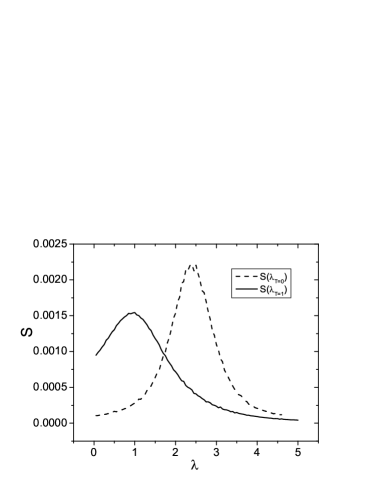
Figure 5: The evolution of ICE: along the line of increasing isovector pairing $\lambda_{T=1}$ at fixed $\lambda_{T=0}=\lambda_{np}=1$,solid line; as a function of $\lambda_{T=0}$ at fixed $\lambda_{T=1}=\lambda_{np}=1$, dashed line. Interval $\delta=0.05$ was used here.

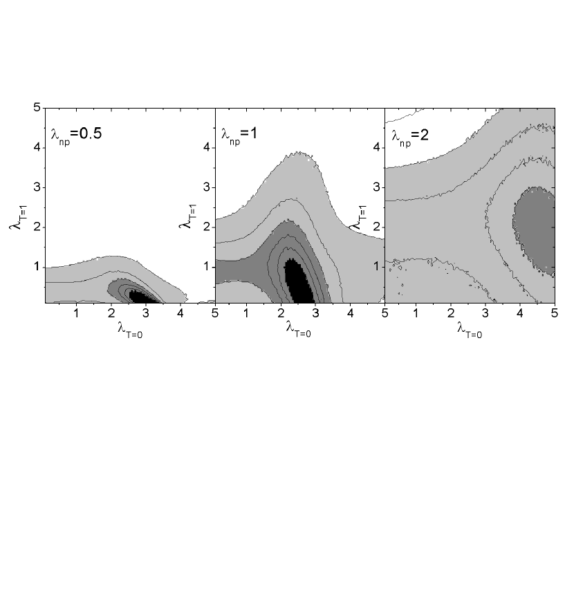
Figure 6: ICE of the ground state in ²⁴Mg computed on the plane $\lambda_{T=0}-\lambda_{T=1}$. The three panels show the evolution of the phase diagram depending on the overall scale of non-pairing matrix elements $\lambda_{np}.$ The averaging interval of $\delta=0.05$ was used, and the entropy is scaled (divided) by 0.015.

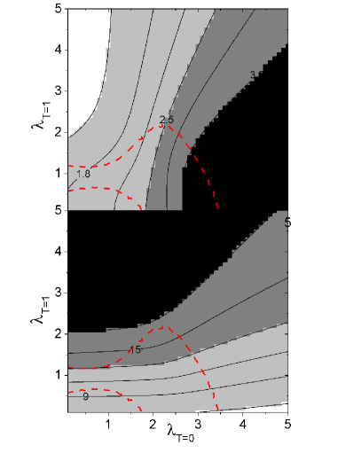
Figure 7: Effective average number of $T=0$ and $T=1$ pairs, upper and lower panels, respectively, for the ground state of ²⁴Mg at $\lambda_{np}=1$ on the $\lambda_{T=0}-\lambda_{T=1}$ plane. The dashed line outlines the regions where ICE is enhanced above 0.45.

As our last example, we consider the $sd$ shell model for ²⁴Mg. At $N=Z$, the competition of isovector, isoscalar, deformation and alpha-particle correlations makes the physical picture very complex. Empirical information macchiavelli00 , studies of simple models evans81 ; dussel86 ; engel97 ; baldini03 ; palchikov01 and analytic works ropke98 , supplemented by the direct shell model diagonalization vogel99 , support the plausible existence of different phases. However, it still remains unclear whether these phases are pure enough to be identified, or whether they are separated by distinct critical regions. Here the ICE provides a helpful tool.

For this example we extend the list of parameters to include $\lambda_{T=1}$, $\lambda_{T=0}$ and $\lambda_{np}$, which scale isovector ($T=1$, $L=0$), isoscalar ($T=0$, $L=1$), and all remaining two-body matrix elements in the Hamiltonian, respectively. The shell model is defined in this example with single-particle energies and interaction matrix elements from Ref. brown88 . In Fig. 5, where ICE is shown as a function of $\lambda_{T=1}$ with $\lambda_{T=0}=\lambda_{np}=1$ as a solid line and as a function of $\lambda_{T=0}$, while $\lambda_{T=1}=\lambda_{np}=1$, as a dashed line, indicates again a phase transition. The contour plot of ICE for this example is shown in Fig. 6. We limit ourselves here to three different strengths of non-pairing interactions $\lambda_{np}=0.5,1,$ and 2. This already gives a general idea of the ICE evolution. The valley in the vicinity of small $\lambda_{T=0}$ and $\lambda_{T=1}$ that corresponds to a normal state is clearly separated, and with increase of the strength of non-pairing interactions this region widens. However, at large $\lambda_{np}$ the sharpness of the phase transition is significantly reduced; note that the scale in the right panel in Fig. 6 is ten times smaller. This effect is analogous to the situation observed in ⁴⁸Ca, where, except for some special area, non-pairing interactions smeared the phase transition region.

The only valley clearly separated by the mountains of ICE corresponds to the normal state. To identify phases of $T=1$ and $T=0$ pairing, similarly to our previous example, we calculate the number of coherent pairs for $\lambda_{np}=1$ case shown in Fig. 7. We consider isovector, $T=1,\,L=0$, and isoscalar, $T=0,\,L=1$, pairs (7). For both limiting cases of pure isovector and isoscalar pairing, ${\cal N}_{T}$ can be calculated using group algebra, see for example engel98 . In the states of degenerate isovector pairing model

$${\cal N}_{1}=\frac{1}{2}\left[\frac{1}{4}(N-s)(\Omega-N-s+6)+{\bf t}^{2}-{\bf T}^{2}\right]\,,$$ (8)

where ${\bf t}$ is isospin of unpaired particles, while ${\bf T}$ is total isospin of the system. Thus, in the state with maximum isovector pairing, $s=0$, ${\bf t}={\bf T}=0$, one would expect ${\cal N}_{1}=N(\Omega-N+6)/8$, which in our case of $N=8$ and $\Omega=24$ leads to ${\cal N}_{1}=22.$ Interchanging angular momentum and isospin and taking normalization of operators into account we obtain ${\cal N}_{0}=N(\Omega-N+6)/(2\Omega)$, which results in maximum ${\cal N}_{0}\approx 3.7,$ whereas statistically $\overline{{\cal N}_{1}}\approx 1.8$ and $\overline{{\cal N}_{0}}\approx 0.3.$ This analysis along with Fig. 7 allow us to confirm the presence of isovector and isoscalar paired states in the upper left and lower right areas of the phase diagram. The isovector pairing phase appears as a shaded area in the lower panel of Fig. 7, and the shaded area of the upper panel indicates the isoscalar pairing state. Furthermore, the enhancement of ICE, the region outlined by a dashed line on both panels of Fig. 7, is consistent with the presence of the phase transition from normal to either of superconducting phases; this is the area of the most rapid rise in the number of coherent pairs ${\cal N}_{0}$ or ${\cal N}_{1}.$

Further examination of Fig. 6 indicates a notable absence of any additional phase transition, as for example between isovector-isoscalar and possibly alpha-clustering phases. Clearly there are no phase separating lines far from the origin, i.e. at large $\lambda_{T=0}$ and $\lambda_{T=1}.$ Thus, a continuous path between isovector and isoscalar phases does not involve a transitional behavior, unlike a transition from the normal state to any paired state.

The point corresponding to the realistic nucleus, $\lambda_{T=1}=\lambda_{T=0}=\lambda_{np}=1$, is located in the transitional region from the normal to isovector pairing phase on the side of the paired state. On the other hand, the isoscalar pairing matrix elements are to be increased by a factor of three to bring the system onto a border between the normal phase and quasideuteron $T=0$ pairing coherence, this seen best from Fig. 5. Our result, that in the $N=Z$ nucleus the $T=1$ pair coherence is enhanced in contrast to $T=0$, is supported by other findings macchiavelli00 ; vogel99 .

Let us summarize the results for our shell model examples. In ⁴⁸Ca we are able to unambiguously identify the pairing phase transition. This nucleus would be in the paired state if no interactions of non-pairing type had been present. The incoherent residual interactions in reality put the ground state below the phase transition line although in the region of large fluctuations preceding the onset of well developed pairing. This explains earlier results volyaEP : the failure of the BCS theory and large pairing correlation energy found in the exact solution. We have also found that the change in non-pairing interactions does not lead to a phase transition, however it influences substantially the normal-to-pairing critical region. Weak residual incoherent interactions smear the phase transition as they facilitate the pair excitation. Strong non-pairing interactions create complexity in dynamics, and a strong phase transition occurs when such system is “cooled” and the superconducting order is established.

Considering the ²⁴Mg nucleus we observed a clear phase transition between the normal and superconducting state. We identified the regions where two different types of pairing, isovector and isoscalar, exist. The ²⁴Mg nucleus is found, in agreement with earlier results, to be in the isovector phase and within the critical region of the normal to superconducting transition. The isoscalar pairing should have been three times stronger compared to the realistic shell model forces in order to lead to the corresponding condensate. Within limited shell model space we found no evidence of a phase transition between different types of pairing or alpha-clustering.

To conclude, in this work we suggested a new theoretical technique for tracking and quantitatively studying the phase transitions in nuclei and, more generally, in mesoscopic systems. Invariant correlational entropy serves not only as an indicator of the degree of complexity along the spectrum big but as a powerful tool for identifying the regions of rapid changes of structure in response to variations in a control parameter, here it was a strength of the interaction. A mesoscopic system is sufficiently large to display statistical regularities but still sufficiently small to allow one to probe, theoretically and experimentally, individual wave functions. Such a system significantly alters the features of phase transitions, and opens a door for “secondary” interactions to leave a noticeable footprint. The ICE clearly shows the sensitive spots of the parameter space.

- (1) S. Sachdev, Quantum phase transitions, Cambridge University Press, 1999.
- (2) P. Borrmann, J. Harting, Phys. Rev. Lett. 86 (2001) 3120.
- (3) O. Mulken, H. Stamerjohanns, P. Borrmann, Phys. Rev. E 64 (2001) 047105.
- (4) V.V. Sokolov, B.A. Brown, V. Zelevinsky, Phys. Rev. E 58 (1998) 56.
- (5) P. Cejnar, V. Zelevinsky, V.V. Sokolov, Phys. Rev. E 63 (2001) 036127.
- (6) F. Izrailev, Phys. Rep. 196 (1990) 299.
- (7) V. Zelevinsky, B.A. Brown, N. Frazier, M. Horoi, Phys. Rep. 276 (1996) 85.
- (8) A. Volya, V. Zelevinsky, B.A. Brown, Phys. Rev. C 65 (2002) 054312.
- (9) A. Rabhi, R. Bennaceur, G. Chanfray, P. Schuck, Phys. Rev. C 66 (2002) 64315.
- (10) A. Volya, B.A. Brown, V. Zelevinsky, Phys. Lett. B 509 (2001) 37.
- (11) P. Cottle, K. Kemper, Phys. Rev. C 66 (2002) 61301.
- (12) T. Werner, J. Sheikh, M. Misu, W. Nazarewicz, J. Rikovska, K. Heeger, A. Umar, M. Strayer, Nucl. Phys. A597 (1996) 327.
- (13) G. Lalazissis, D. Vretenar, P. Ring, M. Stoitsov, L. Robledo, Phys. Rev. C 60 (1999) 014310.
- (14) W. Richter, M. van der Merwe, R. Julies, B.A. Brown, Nucl. Phys. A523 (1991) 325.
- (15) V. Zelevinsky, A. Volya, Phys. Part. Nucl. in press .
- (16) J. Harting, O. Mulken, P. Borrmann, Phys. Rev. B 62 (2000) 10207.
- (17) J. Egido, L. Robledo, V. Martin, Phys. Rev. Lett. 85 (2000) 26.
- (18) A. Macchiavelli at al., Phys. Lett. B 480 (2000) 1; Phys. Rev. C 61 (2000) 041303.
- (19) J. Evans, G. Dussel, E. Maqueda, R. Perazzo, Nucl. Phys. A367 (1981) 77.
- (20) G. Dussel, E. Maqueda, R. Perazzo, J. Evans, Nucl. Phys. A460 (1986) 164.
- (21) J. Engel, S. Pittel, M. Stoitsov, P. Vogel, J. Dukelsky, Phys. Rev. C 55 (1997) 1781.
- (22) E. Baldini-Neto, C. Lima, P. Van Isacker, Phys. Rev. C 65 (2002) 064303.
- (23) Y. Palchikov, J. Dobes, R. Jolos, Phys. Rev. C 63 (2001) 034320.
- (24) G. Ropke, A. Schnell, P. Schuck, P. Nozieres, Phys. Rev. Lett. 80 (1998) 3177.
- (25) G. Martinez-Pinedo, K. Langanke, P. Vogel, Nucl. Phys. A651 (1999) 379.
- (26) B.A. Brown, B. Wildenthal, Ann. Rev. Nucl. Part. Sci. 38 (1988) 29.
- (27) J. Engel, K. Langanke, P. Vogel, Phys. Lett. B 429 (1998) 215.