Transverse momentum dependence of Hanbury Brown-Twiss radii of pions from a perfectly opaque source with hydrodynamic flow

Abstract

We investigate the transverse momentum dependence of pion HBT radii on the basis of a hydrodynamical model. Recent experimental data show that $R_{\text{out}}/R_{\text{side}}<1$, which suggests a strong opaqueness of the source. In addition to the opaqueness naturally caused by transverse flow, we introduce an extrinsic opacity by imposing restrictions on the pion emission angle. Comparing the HBT radii obtained from the normal Cooper-Frye prescription and the opaque emission prescription, we find that $R_{\text{out}}/R_{\text{side}}$ is less than unity only for small values of the transverse momentum with an opaque source. However, HBT radii for large values of the transverse momentum are dominated by the transverse flow effect and are affected less by the source opaqueness.

I Introduction

Pion interferometry is one of the most promising tools for use in high energy heavy ion collision experiments designed to explore the states of matter under extreme conditions. As is well known, the Hanbury Brown-Twiss (HBT) effect, caused by the symmetry of the wave function of identical bosons, provides information concerning the geometry of the source via two-particle intensity correlation functions Weiner_PREP . Recently, the Relativistic Heavy Ion Collider (RHIC) at Brookhaven National Laboratory (BNL) has started to operate at extremely high energies. This opens a new frontier of heavy ion collision experiments. Experimental data obtained at the partial collision energy $\sqrt{s}=130A$ GeV and preliminary data at $\sqrt{s}=200A$ GeV have been reported QM2002 . One of the most interesting but puzzling results is that derived from the pion HBT data STAR_HBT . Usually, the outward HBT radius $R_{\text{out}}$ is believed to be larger than the sideward HBT radius $R_{\text{side}}$ by an amount equal to the duration time, i.e. $R_{\text{out}}^{2}\sim R_{\text{side}}^{2}+\beta_{\bot}^{2}(\Delta t)^{2}$. A hydrodynamical model with a phase transition naively predicts large outward HBT radii around the RHIC energy because of the prolonged lifetime of the fluid due to the existence of the phase transition Hydro_Longtau ; Rischke_NPA608 . The obtained HBT radii in the RHIC experiments, however, reveal the surprising feature that $R_{\text{out}}$ is almost the same as (or even smaller than) $R_{\text{side}}$. The ratio $R_{\text{out}}/R_{\text{side}}$, which is proposed for a good indicator of the long emission duration Rischke_NPA608 , exhibits a slight decrease around unity with the pair transverse momentum. This strange result is sometimes called the “HBT puzzle”.

Let us briefly survey the present situation regarding HBT radii. The collision process is governed by strong and multi-body interactions, including multiparticle production. At this time, we are far from the dynamical description of the entire process in terms of the fundamental theory. Though pions possess information only at their freeze-out, because of the strong interaction, the two-pion correlation function provides the space-time distribution of the freeze-out point and the history of the space-time evolution, which is subject to the equation of state. Therefore, a dynamical model is indispensable for understanding the HBT data, and a hydrodynamical approach is quite suitable for this purpose. In addition, recent experimental data concerning an anisotropic flow ($v_{2}$) obtained in the mid-rapidity region strongly support the validity of the hydrodynamical picture at the energies typically studied with the RHIC Kolb_PLB500 . However, conventional hydrodynamical model analyses that reproduce single-particle spectra (and elliptic flow in Ref. Heinz_NPA702 ) result in unsatisfactory HBT radii Heinz_NPA702 ; Morita_PRCRapid . Space-time evolution with a smooth crossover transition equation of state provides a small improvement, but the resulting predictions for the HBT radii are still far from agreeing with the data Zschiesche_PRC65 . Though smaller HBT radii can be obtained, especially in the longitudinal direction, by introducing the chemical freeze-out in addition to the thermal freeze-out Hirano_PRC66 (see also Ref. Kolb_PRC67 ), this decrease is still insufficient to account for the experimental results. Some transport calculations indicate that the creation of dense partonic matter has a tendency to improve the HBT radii Lin_PRL89 . The problem will be the description of the hadronic stage and the subsequent freeze-out. A possible solution of this problem may be to introduce a modification of the freeze-out hypersurface in hydrodynamical models, on which the number of the emitted particle is usually carried out by using the Cooper-Frye prescription Cooper_Frye with a sharp three-dimensional hypersurface. A more sophisticated treatment of the freeze-out combined with the hadronic transport calculation is still not sufficient to obtain predictions consistent with experiment Soff_PRL .

Considering the meaning of the HBT radii given by second order moments of the emission function Chapman_PRL74 , the experimentally obtained results that $R_{\text{out}}\sim R_{\text{side}}$ indicate an “opaque source” Heiselberg_EPJC1 ; Tomasik_nucl9805016 , from which particles are emitted only on a thin surface. It has been shown that transverse flow in the hydrodynamic evolution also naturally causes opaque features of the HBT radii Morita_PRC , and such effects are already automatically taken into account in the calculation. However, this effect is not sufficient to realize consistency with the experimental data. Therefore, we must introduce additional mechanisms that increase the source opacity. In the present paper, we investigate the HBT radii on the bases of a hydrodynamical model Morita_PRCRapid . By putting a restriction on the emission angle of pions, we introduce complete opaqueness of the source given by the hydrodynamical model. Comparing the HBT radii obtained from normal emission with those from this opaque source model, we study the transverse momentum dependence of the HBT radii and clarify its origin.

In the next section, we briefly explain our model. In $\S$III, a description of the opaque source model is given. Section IV is devoted to results and discussion.

II Model

We describe the space-time evolution of hot matter created in $\sqrt{s}=200A$ GeV Au+Au central collisions at the RHIC using the hydrodynamical model presented in Ref. Morita_PRCRapid . We can fit single-particle distributions of charged hadrons, such as the pseudorapidity distribution from the PHOBOS collaboration PHOBOS_dndeta200 , the net-proton rapidity distribution from the BRAHMS collaboration BRAHMS_netproton , and the identified transverse momentum distributions from the PHENIX collaboration PHENIX_pt , by adjusting parameters in the initial matter distributions. Here, we adopt the following functional form of the initial net baryon number distribution:

$$n_{\text{B}}(\tau_{0},\eta,r)=n_{\text{B0}}\left\{\exp\left[-\frac{(|\eta|-\eta_{\text{D}})^{2}}{2\sigma_{\text{D}}^{2}}\right]\theta(|\eta|-\eta_{0})+\exp\left[-\frac{(\eta_{0}-\eta_{\text{D}})^{2}}{2\sigma_{\text{D}}^{2}}\right]\theta(\eta_{0}-|\eta|)\right\}$$

$$\times\exp\left[-\frac{(r-r_{0})^{2}}{2\sigma_{r}^{2}}\theta(r-r_{0})\right].$$ (1)

This form is employed in order to reproduce the flat net-proton distribution for $|y|~{}\leq~{}1$ obtained by the BRAHMS collaboration BRAHMS_netproton ,  The parameter set is listed in Table. 1. The particle distributions are calculated using the Cooper-Frye prescription Cooper_Frye . We also take into account the resonance decay contribution, as in Ref. Morita_PRCRapid . Note that our calculation does not reproduce absolute numbers of kaons and (anti-)protons, because we assume the single freeze-out condition. Incorporating chemical freeze-out Hirano_PRC66 ; Teaney_nucl0204023 ; Kolb_PRC67 , or an additional assumption for the initial stage that leads to stronger transverse flow Eskola_hep0206230 , makes it possible to reproduce both the $p_{\text{T}}$ slope and the yield of each particle species. But such modifications do not affect our main argument below.

Table 1: Parameter set for 200$A$ GeV Au+Au collisions at RHIC.

$\varepsilon_{\text{max}}$	$n_{\text{B0}}$	$\eta_{0}$	$\sigma_{r}$	$\sigma_{\eta}$	$\eta_{D}$	$\sigma_{D}$	$T_{\text{f}}$
6.9 GeV/fm3	0.22 fm-3	1.3	1.0 fm	1.4	2.6	0.92	130 MeV

III Two-pion correlation function from an opaque source

The two-pion intensity correlation function for a chaotic source is given by Shuryak_PLB44

$$C_{2}(q,K)=1+\frac{|I(q,K)|^{2}}{I(0,k_{1})I(0,k_{2})}$$ (2)

where $k_{1}$ and $k_{2}$ are the on-shell four-momenta of the two emitted pions, and $q$ and $K$ are the relative and average four-momentum defined as $q=k_{1}-k_{2}$ and $K=(k_{1}+k_{2})/2$, respectively. We choose $I(q,K)$ as

$$I(q,K)=\int_{\Sigma}K\cdot d\sigma(x)e^{iq\cdot x}f(x,K),$$ (3)

where $f(x,K)$ is the Bose-Einstein distribution function $[\exp(K\cdot U(x)/T(x))-1]^{-1}$, so that $I(0,k)$ reduces to the Cooper-Frye formula of a single-particle distribution Chapman_PLB340 . Note that $K$ is the off-shell four-momentum, and $\Sigma$ denotes that the integration is carried out over the 3-dimensional freeze-out hypersurface determined by $T=T_{\text{f}}$.

Figure 1: A schematic view of the freeze-out hypersurface (thick curve) in the $r$-$t$ plane ($\eta=0$) and the directions (arrows) of emitted particles. (a) and (b) are allowed directions, but (c) is forbidden.

As mentioned in $\S$I, the opaqueness of the source represents a possible solution of the HBT puzzle. Here, we introduce a simple opaque source model by imposing two conditions on the emission from the freeze-out hypersurface.

The first condition is the space-time geometrical constraint that a particle can not be emitted into the fluid; i.e., “inward” emission is forbidden. The assumption of local thermal equilibrium implies isotropic particle emission in the local rest frame of a fluid element. Therefore, inward emission naturally occurs even after a Lorentz boost to the center-of-mass system, though its contribution to the multiplicity is known to be small. In the Cooper-Frye freeze-out prescription, the number of particles absorbed from time-like surfaces can be considered as negative Sinyukov_ZPHYS43 ; Bernard_NPA605 ; Bugaev_NPA606 ; Anderlik_PRC59 . We omit such emissions by introducing the step function $\theta(p\cdot d\sigma)$ for $p=k_{1}$ and $k_{2}$ in the surface integrations. (See also Fig. 1.)

The second condition is a purely three-dimensional geometrical constraint that is characterized by the factor $\theta(\cos(\phi-\psi))$, where $\phi=\tan^{-1}(r_{y}/r_{x})$ is the azimuthal angle of the emission point, $\psi=\tan^{-1}(k_{y}/k_{x})$ is the azimuthal emission angle of the particle (Fig. 2), and $\theta$ is the step function. This constraint prohibits the emissions in the direction opposite to the radial flow velocity, which occur naturally by virtue of the assumption of the local thermal equilibrium. For example, for a particle with $k_{x}=k_{\text{T}}$ and $k_{y}=0$, we allow emissions from space-time points at $r_{x}>0$, which corresponds to the limited range of azimuthal angles of emission points $-\pi/2\leq\phi\leq\pi/2$ . Hence, we regard the source constructed with these two conditions as a perfectly opaque source, from which particles cannot be emitted from the side opposite to the detector.

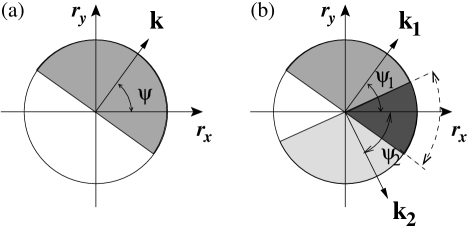
Figure 2: Emission angle constraint in $x$-$y$ plane. In (a), the filled region represents the allowed region that satisfies the constraint. Figure (b) describes the two-particle case, where the overlapping area indicated by the darkest shading is that in which the constraint is satisfied for both particles.

Note that the above constraints should be imposed on each particle, while the two-particle correlation function can be expressed as the Fourier transform of the (pseudo-) single-particle distribution function. (See also Fig. 2(b).) Therefore, we input the constraints on each emitted particle into both numerator and denominator of Eq. (2) as

$$C_{2}(q,K)=1+\frac{\displaystyle\left|\int_{\Sigma}K\cdot d\sigma f(x,K)e^{iq\cdot x}\Theta(x,k_{1})\Theta(x,k_{2})\right|^{2}}{\displaystyle\int_{\Sigma}k_{1}\cdot d\sigma f(x,k_{1})\Theta(x,k_{1})\int_{\Sigma}k_{2}\cdot d\sigma^{\prime}f(x^{\prime},k_{2})\Theta(x^{\prime},k_{2})}$$ (4)

where $\Theta(x,k_{i})\equiv\theta(k_{i}\cdot d\sigma)\theta[\cos(\phi-\psi_{i})]$ and $\psi_{i}=\tan^{-1}(k_{iy}/k_{ix})$ for $i=1,2$. Under these constraints, energy conservation between the fluid and emitted particles through the freeze-out process is violated. We have estimated the loss of energy in a system with the conditions described above to be 11%. This means that 89% of emitted energy quanta satisfy the conditions. The resultant multiplicity $dN/d\eta_{p}$ at $\eta_{p}=0$, where $\eta_{p}$ denotes the pseudorapidity $\eta_{p}=0.5\ln[(|\boldsymbol{p}|+p_{z})/(|\boldsymbol{p}|-p_{z})]$, decreases from 618 to 593. This loss can be considered negligible for the discussion below. Some attempts have been made to avoid this kind of violation by improving the freeze-out prescription Anderlik_PRC59 , but it would be a formidable task to incorporate both the constraints and the conservation low in a self-consistent manner, and this is beyond the scope of this paper.

IV Results and discussions

The HBT radii are obtained through a 3-dimensional $\chi^{2}$-fit to the correlation functions (2) with the form

$$C_{\text{2fit}}(q,K)=1+\exp[-R_{\text{side}}^{2}(K)q_{\text{side}}^{2}-R_{\text{out}}^{2}(K)q_{\text{out}}^{2}-R_{\text{long}}^{2}(K)q_{\text{long}}^{2}].$$ (5)

Figure 3: HBT radii for 200$A$ GeV Au+Au collisions as functions of the averaged transverse momentum $K_{\text{T}}$. From top to bottom, the open squares represent the results from our model with normal freeze-out, given by Eqs. (2) and (3). The results from opaque freeze-out [Eq. (4)] are represented by the open circles. The solid circles and squares represent the STAR and PHENIX experimental results, respectively.

In this section, we compare the “normal” HBT radii calculated using Eqs. (2) and (3) and the “opaque” case calculated using Eq. (4). We focus on $R_{\text{out}}$ and $R_{\text{side}}$, because the purpose of this paper is to clarify the effects of the transverse dynamics, i.e., the flow effect and opacity effect. $R_{\text{long}}$ does not reflect such effects, because its $K_{\text{T}}$ dependence originates mainly from rapid longitudinal expansion Hama_PRD37 . In the numerical evaluation of the correlation function, the experimental window effect was simply ignored for the better understanding of the opacity effect. The following approximate expressions for the HBT radii in terms of second-order moments of the source function are convenient Chapman_PRC :

$$R_{\text{side}}^{2}(\boldsymbol{k}) =\langle\tilde{r_{y}}^{2}\rangle,$$ (6)

$$R_{\text{out}}^{2}(\boldsymbol{k}) =\langle(\tilde{r_{x}}-\beta_{\perp}\tilde{t})^{2}\rangle$$

$$=\langle\tilde{r_{x}}^{2}\rangle-2\beta_{\perp}\langle\tilde{r_{x}}\tilde{t}\rangle+\beta_{\perp}^{2}\langle\tilde{t}^{2}\rangle.$$ (7)

Here,

$$\langle A(x)\rangle(\boldsymbol{k})\equiv\frac{\displaystyle\int_{\Sigma}k\cdot d\sigma f(x,k)A(x)}{\displaystyle\int_{\Sigma}k\cdot d\sigma f(x,k)},$$ (8)

where $\tilde{x}\equiv x-\langle x\rangle$ and $\beta_{\perp}=k_{\text{T}}/E_{\boldsymbol{k}}$. These are good approximation for both of the emission prescriptions.

Figure 3 displays the results for HBT radii together with recent preliminary experimental results from the STAR STAR_HBT200 and the PHENIX PHENIX_HBT200 obtained from $\sqrt{s}=200A$ GeV Au+Au collisions.

Figure 4: $r_{x}$-$t$ correlations and source width in the outward ($x$) direction.

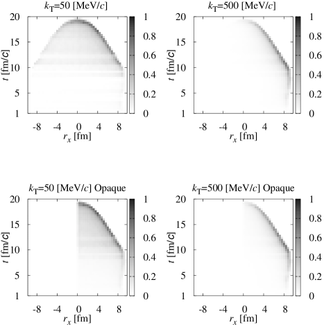
Figure 5: Source function in the $r_{x}$-$t$ plane. The upper graphs are for the case of the normal freeze-out procedure, and the lower ones are for the opaque emission case. For each freeze-out, the small transverse momentum case ($k_{\text{T}}$ = 50 MeV/$c$, left row) and large transverse momentum case ($k_{\text{T}}$ = 500 MeV/$c$, right row) are presented.

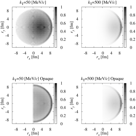
Figure 6: Source function in the $r_{x}$-$r_{y}$ plane. As in the previous figure, the normal and opaque emission cases are considered for $k_{\text{T}}$ = 50 MeV/$c$ and 500 MeV/$c$, respectively.

The results of the normal freeze-out prescription exhibit deviations similar to those seen in the 130$A$ GeV results Morita_PRCRapid . In particular, $R_{\text{side}}$ is smaller and decreases less steeply with increasing $K_{\text{T}}$, $R_{\text{out}}$ is larger, and $R_{\text{out}}/R_{\text{side}}$ is much larger, which corresponds to a long emission duration due to the phase transition. Despite the strong restriction on the emission direction by Eq. (4), only a slight improvement of $R_{\text{side}}$ and $R_{\text{out}}$ is seen. In the opaque source model, $R_{\text{side}}$ becomes larger at small $K_{\text{T}}$, and its $K_{\text{T}}$ dependence becomes slightly steeper than in the normal emission case. $R_{\text{out}}$ becomes slightly smaller at small $K_{\text{T}}$, though no improvement can be seen beyond $K_{\text{T}}\sim 0.5$ GeV/$c$. Consequently, the ratio of $R_{\text{out}}$ to $R_{\text{side}}$ improves to a value less than unity in the smallest $K_{\text{T}}$ bin. Nevertheless, in the larger $K_{\text{T}}$ region, the opaque emission does not yield results consistent with the experimental data. These results suggest that the emission angle restriction does not affect the correlation function at larger $K_{\text{T}}$. After all, the flow effect dominates in this region. This fact can be intuitively understood by calculating $r_{x}$-$t$ correlations and $\langle\tilde{r_{x}}^{2}\rangle$ (Fig. 4) and by plotting the source functions in the $r_{x}$-$t$ (Fig. 5) and $r_{x}$-$r_{y}$ (Fig. 6) planes. The source functions are calculated as

$$S_{xt}(r_{x},t;k_{\text{T}}) =*\int_{|\eta|\leq 1}k\cdot d\sigma(x^{\prime})f(x^{\prime},k)\delta(r_{x}-r_{x}^{\prime})\delta(t-t^{\prime}),$$ (9)

$$S_{xy}(r_{x},r_{y};k_{\text{T}}) =*\int k\cdot d\sigma(x^{\prime})f(x^{\prime},k)\delta(r_{x}-r_{x}^{\prime})\delta(r_{y}-r_{y}^{\prime}).$$ (10)

Each function is calculated at mid-rapidity and is normalized such that its maximum value is unity. For $S_{xt}(r_{x},t;k_{\text{T}})$, integration over the space-time rapidity $\eta\equiv 0.5\ln[(t+z)/(t-z)]$ is carried out with $|\eta|\leq 1$ in order to obtain a clear emission probability distribution. For the opaque emission model, $\Theta(x,k)$ is inserted into the above definitions as in Eq. (4).

Figure 4 reveals a large decrease of $\Delta r_{x}=\sqrt{\langle\tilde{r_{x}}^{2}\rangle}$ at small $k_{\text{T}}$ in the opaque emission model, as expected. This behavior is clearly caused by the emission angle restriction factor $\theta(\cos(\phi-\psi_{i}))$, which cuts off emission from $x<0$ for $k_{\text{T}}=(k_{\text{T}},0)$, as seen from the left column ($k_{\text{T}}=50$ MeV/$c$) of Fig. 6. However, such a distinct difference disappears at higher $k_{\text{T}}$, because the flow causes a strong suppression and enhancement through the Boltzmann factor (right column). Thus, as $k_{\text{T}}$ increases, the relative effect of opacity becomes weaker in the presence of transverse flow. Another factor, $-2\beta_{\bot}\langle\tilde{r_{x}}\tilde{t}\rangle$, in $R_{\text{out}}$ exhibits strong dependence on $k_{\text{T}}$, as seen in Fig. 4, though it does not affect $R_{\text{out}}$ greatly. In the $k_{\text{T}}$ region satisfying $(\Delta r_{x})_{\text{opaque}}\ll(\Delta r_{x})_{\text{normal}}$, the prefactor $\beta_{\bot}$ is so small that the second term of Eq. (7) gives only a small contribution to $R_{\text{out}}$. The decrease of $\langle\tilde{r_{x}}\tilde{t}\rangle$ in the opaque emission model is due to the larger $\langle r_{x}\rangle$, which is a natural consequence of emission only from the region $r_{x}>0$. The leading contribution in this region, however, is $\Delta t$, which is 6 fm$/c$ for $k_{\text{T}}=200$ MeV/$c$ (Fig. 7). Therefore, the reduction of $\langle\tilde{r_{x}}\tilde{t}\rangle$ does not reduce $R_{\text{out}}$ so much. From Fig. 6, some increase of the emissivity at the edge can be seen due to the cutoff of time-like surface emission. (Also, as seen from Fig. 1, surface elements at the edge naturally have a time-like part.) This fact results in the slight increase of $R_{\text{side}}$ for small $k_{\text{T}}$, because $R_{\text{side}}$ can be considered the width of the source along the $y$ direction.

Figure 7: $R_{\text{out}}$ calculated from Eq. (7) and the time duration, $\Delta t$.

In the present paper, we have demonstrated that a naive opaque emission model in which we forbid emissions through dense media does not account for the “HBT puzzle” if collective transverse flow exists. The opaqueness caused by the dense matter preventing the pions from passing through such media affects the HBT radii only at small transverse momentum. As a result, smaller values of $R_{\text{out}}$ than $R_{\text{side}}$ are obtained only for small $k_{\text{T}}$. Incorporating the opacity effect transforms the shape of the source function. Nevertheless, transverse flow dominates the source function for large $k_{\text{T}}$; modification of the source function by the opacity is so slight that the $k_{\text{T}}$ dependence of the HBT radii is still dominated by the transverse flow effect.

As mentioned above, the present study constitutes a trial studying the modification of the source shape. One can consider other possibilities. For example, a viscosity correction Teaney_QM02 and $\rho$ meson broadening Soff_QM02 have been examined. It also should be noted that a thermal model analysis yields acceptable agreement Broniowski_HBT . This agreement results from the fact that their model used in that study has a positive $r_{x}$-$t$ correlation due to the choice of the freeze-out hypersurface. However, that surface was simply added by hand, and is not the result of a dynamical calculation. Further investigation is required to solve the puzzle.

References

-
(1)
R. M. Weiner, Phys. Rep. 327, 249 (2000).
U. A. Wiedemann and U. Heinz, Phys. Rep. 319, 145 (1999).
B. Tomášik and U. A. Wiedemann, hep-ph/0210250. - (2) Quark Matter 2002, Proceedings of the 16th International Conference on Ultra-Relativistic Heavy Ion Collisions eds. H. Gutbrod, J. Aichelin and K. Werner (North-Holland, 2003); Nucl. Phys. A715,1c (2003).
-
(3)
C. Adler et al. (STAR Collaboration),
Phys. Rev. Lett. 87, 082301 (2001).
K. Adcox et al. (PHENIX Collaboration), Phys. Rev. Lett. 88, 192302 (2002). - (4) P. F. Kolb, P. Huovinen, U. Heinz and H. Heiselberg, Phys. Lett. B500, 232 (2001).
-
(5)
H. von Gersdorff, L. McLerran, M. Kataja and P. V. Ruuskanen,
Phys. Rev. D34, 794 (1986).
M. Kataja, P. V. Ruuskanen, L. McLerran and H. von Gersdorff, Phys. Rev. D34, 2755 (1986).
S. Pratt, Phys. Rev. D33, 1314 (1986).
However, a long lifetime does not directly mean the existence of the phase transition, see also T. Ishii and S. Muroya, Phys. Rev. D46, 5156 (1992). - (6) D. H. Rischke and M. Gyulassy, Nucl. Phys. A608, 479 (1996).
- (7) U. Heinz and P. Kolb, Nucl. Phys. A702, 269 (2002).
- (8) T. Hirano, K. Morita, S. Muroya and C. Nonaka, Phys. Rev. C65, 061902 (2002); K. Morita, S. Muroya, C. Nonaka and T. Hirano, ibid. 66, 054904 (2002).
- (9) D. Zschiesche, H. Stöcker, W. Greiner and S. Schramm, Phys. Rev. C65, 064902 (2002).
- (10) T. Hirano and K. Tsuda, Phys. Rev. C66, 054905 (2002).
- (11) P. F. Kolb and R. Rapp, Phys. Rev. C67, 044903 (2003).
- (12) K. Adcox et al. (PHENIX Collaboration), Phys. Rev. Lett.88, 022301 (2002).
-
(13)
Z. Lin, C. M. Ko and S. Pal,
Phys. Rev. Lett.89, 152301 (2002).
D. Molnár and M. Gyulassy, nucl-th/0211017. - (14) F. Cooper and G. Frye, Phys. Rev. D10, 186 (1974).
-
(15)
S. Soff, S. A. Bass and A. Dumitru,
Phys. Rev. Lett.86, 3981 (2001).
S. Soff, S. A. Bass, D. H. Hardtke and S. Y. Panitkin, ibid. 88, 072301 (2002). - (16) S. Chapman, P. Scotto and U. Heinz, Phys. Rev. Lett.74, 4400 (1995).
- (17) H. Heiselberg and A. P. Vischer, Eur. Phys. J. C1, 593 (1998).
- (18) B. Tomášik and U. Heinz, nucl-th/9805016.
- (19) K. Morita, S. Muroya, H. Nakamura and C. Nonaka, Phys. Rev. C61, 034904 (2000).
- (20) L. McLerran and S. S. Padula, hep-ph/0205028.
- (21) B. B. Back et al. (PHOBOS Collaboration), Phys. Rev. Lett.91, 052303 (2003).
- (22) P. Christiansen (BRAHMS Collaboration), to appear in the proceedings of 16th International Conference on Particles and Nuclei (PANIC 02), Osaka, Japan, 30 Sep - 4 Oct 2002; nucl-ex/0212002.
- (23) T. Chujo (PHENIX Collaboration), Nucl. Phys. A715, 151c (2003).
- (24) D. Teaney, nucl-th/0204023.
- (25) K. J. Eskola, H. Niemi, P. V. Ruuskanen and S. S. Räsänen, Phys. Lett. B566, 187 (2003).
- (26) E. V. Shuryak, Phys. Lett. 44B, 387 (1973).
- (27) S. Chapman and U. Heinz, Phys. Lett. B340, 250 (1994).
- (28) Y. M. Sinyukov, Z. Phys. C43, 401 (1989).
- (29) S. Bernard, J. A.Maruhn, W. Greiner and D. H. Rischke, Nucl. Phys. A605, 566 (1996).
- (30) K. A. Bugaev, Nucl. Phys. A606, 559 (1996).
- (31) C. Anderlik, L. P. Csernai, F. Grassi, W. Greiner, Y. Hama, T. Kodama, Z. I. Lázár, V. K. Magas and H. Stöcker, Phys. Rev. C59, 3309 (1999).
-
(32)
Y. Hama and S. S. Padula, Phys. Rev. D37, 3237 (1988).
A. N. Makhlin and Y. M. Sinyukov, Z. Phys. C39, 69 (1988). - (33) S. Chapman, J. R. Nix and U. Heinz, Phys. Rev. C52, 2694 (1995).
- (34) M. L. Noriega (STAR Collaboration), Nucl. Phys. A715, 623c (2003).
- (35) A. Enokizono (PHENIX Collaboration), Nucl. Phys. A715, 595c (2003).
- (36) D. Teaney, Nucl. Phys. A715, 817c (2003).
- (37) S. Soff, S. A. Bass, D. H. Hardtke and S. Y. Panitkin, Nucl. Phys. A715, 801c (2003).
- (38) W. Broniowski, A. Baran and W. Florkowski, AIP Conf. Proc.660, 85 (2003).
- (39) A. Enokizono (PHENIX Collaboration), talk given at the Autumn Meeting of JPS, Miyazaki, September 11, 2003.