The Deuteron as a Canonically Quantized Biskyrmion

Abstract

The ground state configurations of the solution to Skyrme’s topological soliton model for systems with baryon number larger than 1 are well approximated with rational map ansätze, without individual baryon coordinates. Here the canonical quantization of the baryon number 2 system, which represents the deuteron, is carried out in the rational map approximation. The solution, which is described by the six parameters of the chiral group SU(2)$\times$SU(2), is stabilized by the quantum corrections. The matter density of the variational quantized solution has the required exponential large distance falloff and the quantum numbers of the deuteron. Similarly to the axially symmetric semiclassical solution, the radius and quadrupole moment are, however, only about half as large as the corresponding empirical values. The quantized deuteron solution is constructed for representations of arbitrary dimension of the chiral group.

I Introduction

The classical ground state solutions to Skyrme’s topological soliton model for baryons skyrme , with baryon number ($B$) larger than 1, have intriguing geometrical structure, with polyhedral symmetry Battye97 . The simplest example is the system with $B=2$, which has axial symmetry Manton97 , in agreement with the description of the deuteron based on a quantum mechanical Hamiltonian for the interacting two-nucleon system Sick2001 . Simple rational map ansätze, which provide remarkably accurate approximations to the classical ground state configurations, have been derived for several systems with baryon number larger than 1 Houghton98 . These rational maps represent formal generalizations of Skyrme’s hedgehog ansatz for the single baryon. Here the rational map ansatz for the $B=2$ skyrmion is employed to carry out the canonical quantization of the $B=2$ solution, which represents the deuteron.

The Lagrangian density of the Skyrme model is chirally symmetric under constant SU(2)$\times$SU(2) transformations. The parameters of this symmetry group are treated as the collective dynamical coordinates in the quantization procedure.

The semiclassical quantization procedure developed in ref. Adkins83 for the nucleon employs only that half of the parameters of full chiral symmetry group, which correspond to the diagonal subgroup, and therefore it describes only baryons with equal spin and isospin. The description by the SU(2) Skyrme model of such states, which have unequal spin and isospin as the deuteron, requires six dynamical variables in order to allow consideration of separate rotation of the generators of the SU(2) group and the spatial vectors Braaten88 .

Because the generators are irreducible tensors, these rotations are not independent, however, and therefore cannot be not be used for canonical quantization. In the semiclassical quantization procedure the classical skyrmion is treated as a rigid body with the consequence that the quantum mechanical rotation contributes only positive terms to the energy functional. There is then no stable variational solution to the quantized Hamiltonian. To obtain a stable variational quantized solution one may draw on the canonical quantization procedure, which has been developed by K. Fujii et al. Fujii87 for the SU(2) Skyrme model. The treatment of the dynamical field variables of the Skyrme Lagrangian density as quantum-mechanical variables ab initio generates negative quantum corrections and also stable quantum solitons Acus98 . These energy of these quantum solitons depends on the dimension of the representation of the symmetry group in contrast to the semiclassical case Norvaisas94 ; No97 .

The canonical quantization procedure developed below employs the two sets of three Euler angles, which correspond to left and right chiral rotation groups as the six collective coordinates. The resulting canonical angular momentum operators lead to compact forms for both the Lagrangian and Hamiltonian of the biskyrmion. The two sets of independent angular momentum operators allow construction of the eigenstate of the biskyrmion from the eigenstates of two subsystems. For the deuteron the subsystems are the neutron and proton, which form the state with common spin $S=1$ and isospin $T=0$. The approach generalizes to dibaryons, which may be constructed from neutrons and protons as well as from $\Delta$ resonances.

The matter density of the quantum soliton falls off exponentially at long range in contrast to power law falloff of the classical solution. The inverse of the length scale of this exponential falloff for the $B=1$ skyrmion corresponds to the pion mass Acus98 . In the case of the deuteron it should correspond to $2\sqrt{m_{N}B}$, where $B$ is the binding energy and $m_{N}$ the nucleon mass. It is shown here numerically in the rational map approximation that for the variational ground state the matter density falls off at roughly this rate, as required.

The approximate quantum soliton for the deuteron derived here describes the rotational quantum corrections appropriately, but not the large distance solution of two well separated single skyrmions. This is revealed by the magnitude of its radius and quadrupole moment, which are only about half as large as the corresponding empirical values. The semiclassical solution shares these features Braaten88 .

The present manuscript is organized as follows. In Section 2 the classical rational map ansatz for soliton with baryon number $2$ is generalized to representations of arbitrary dimension. In Section 3 this soliton (biskyrmion) is canonically quantized with six collective variables, which correspond to the parameters of chiral symmetry SU(2)$\times$SU(2) group. The expressions for the electric form factor, quadrupole moment and rms radius of the deuteron are presented in Section 4. The numerical results for deuteron observables are discussed in Section 5.

II The classical axisymmetric soliton

The Skyrme model is a Lagrangian density for a unitary field $U(\bm{x},t)$, which may described by any representation of the $SU(2)$ group. In a general reducible representation the most compact expression of the unitary field $U({\bf x},t)$ is as a direct sum of Wigner’s $D$ matrices for the irreducible representations of arbitrary integer or half integer dimension $j$ Norvaisas94 :

$$U(\bm{x},t)=\sum_{j}\oplus D^{j}(\bm{\alpha}(\bm{x},t)).$$ (1)

The $D$ matrices depend on three unconstrained Euler angles $\bm{\alpha}=(\alpha^{1},\alpha^{2},\alpha^{3})$.

The chirally symmetric Lagrangian density has the form

$${\cal L}[U(\bm{x},t)]=-{\frac{f_{\pi}^{2}}{4}}\mathrm{Tr}\{R_{\mu}R^{\mu}\}+{\frac{1}{32e^{2}}}\mathrm{Tr}\{[R_{\mu},R_{\nu}]^{2}\},$$ (2)

where the ”right” current is defined as

$$R_{\mu}=(\partial_{\mu}U)U^{\dagger},$$ (3)

and $f_{\pi}$ (the pion decay constant) and $e$ are parameters.

The static variational solutions to classical Skyrme model for baryon number $B=2$ (biskyrmion) have been derived numerically in refs.Manton97 ; Braaten88 . In ref.Houghton98 the following simple rational map ansatz, which preserves the axial symmetry of ground state solution for the biskyrmion, was found to give an approximation to the ground state energy, with an accuracy of better than 3 per cent:

$$\mathrm{e}^{\mathrm{i}\left(\hat{\bm{n}}\cdot\bm{\sigma}\right)F_{R}(r)}\Longrightarrow U_{R}(\bm{r})={\mathrm{exp}}\{\mathrm{i}\hat{n}^{a}\cdot\hat{J}_{a}F_{R}(r)\}.$$ (4)

Here $\hat{J}_{a}$ are SU(2) generators, which may be defined in representations of arbitrary dimension. The scalar function $F_{R}(r)$ is the ”chiral angle” for the biskyrmion, which is determined by the variational equation of motion. The circular components of the unit vector $\hat{\bm{n}}$ are

$$\hat{n}_{+1} =-\hat{n}^{-1}=-\frac{\sin^{2}\vartheta}{\sqrt{2}\left(1+\cos^{2}\vartheta\right)}\mathrm{e}^{2\mathrm{i}\varphi},$$

$$\hat{n}_{0} =\hat{n}^{0}=\frac{2\cos\vartheta}{1+\cos^{2}\vartheta},$$ (5)

$$\hat{n}_{-1} =-\hat{n}^{+1}=\frac{\sin^{2}\vartheta}{\sqrt{2}\left(1+\cos^{2}\vartheta\right)}\mathrm{e}^{-2\mathrm{i}\varphi}.$$

Substitution of the ansatz (4) in the Lagrangian density (2) yields the following expression for the mass density of the classical biskyrmion:

$$\mathcal{M}_{cl}= \frac{N}{2}\Bigl{\{}f_{\pi}^{2}\bigl{[}F_{R}^{\prime 2}(r)+2\mathcal{I}\sin^{2}F_{R}(r)\bigr{]}$$ (6)

$$+\frac{2\mathcal{I}}{e^{2}}\sin^{2}F_{R}(r)\bigl{[}F_{R}^{\prime 2}(r)+\frac{\mathcal{I}}{2}\sin^{2}F_{R}(r)\bigr{]}\Bigr{\}}.$$

Here $\mathcal{I}$ is the Gaussian curvature, defined as

$$\mathcal{I}=\frac{4\sin^{2}\vartheta}{r^{2}(1+\cos^{2}\vartheta)^{2}}.$$ (7)

In contrast to the hedgehog ansatz for $B=1$ this mass density depends on both the polar angle $\vartheta$ and the radius $r$. The classical Lagrangian density depends on representation only through the overall factor $N=\frac{2}{3}\sum_{j}j(j+1)(2j+1)$, where $2j+1$ is the dimension of the representation, and which may be absorbed by renormalization of the model parameters Norvaisas94 .

The requirement that the soliton mass be stationary yields the following differential equation for the chiral angle:

$$F_{R}^{\prime\prime}(\tilde{r})\left(\tilde{r}^{2}+4\sin^{2}{F_{R}(\tilde{r})}\right) +2F_{R}^{\prime 2}(\tilde{r})\sin{2F_{R}(\tilde{r})}+2\tilde{r}F_{R}^{\prime}(\tilde{r})$$

$$-\sin 2F_{R}(\tilde{r})\bigl{(}2{\tilde{r}^{2}}+\bigl{(}\frac{8}{3}+\pi\bigr{)}\sin^{2}F_{R}(\tilde{r})\bigr{)}=0.$$ (8)

Here the dimensionless variable $\tilde{r}$ is defined as $\tilde{r}=ef_{\pi}r$. At large distances $\tilde{r}\rightarrow\infty$ this equation reduces to the asymptotic form

$$\tilde{r}^{2}F_{R}^{\prime\prime}(\tilde{r})+2\tilde{r}F_{R}^{\prime}(\tilde{r})-4F_{R}(\tilde{r})=0.$$ (9)

The solution to the asymptotic equation (9) falls of with an algebraic power of distance:

$$F_{R}(\tilde{r})=C\tilde{r}^{-\frac{1+\sqrt{17}}{2}}.$$ (10)

The falloff rate is somewhat larger for the biskyrmion than for the hedgehog ansatz for $B=1$, as the power of $\tilde{r}$ in Eq. (10) is $-2.56$ , whereas in the case of $B=1$ it is $-2$. After renormalization by the factor $N$, the biskyrmion baryon density takes the form

$$\mathcal{B}^{0}(r)=-\frac{\mathcal{I}}{2\pi^{2}}F_{R}^{\prime}(r)\sin^{2}F_{R}(r).$$ (11)

III Canonical quantization with six collective variables

The Skyrme Lagrangian (2) is symmetric under chiral SU(2)$\times$SU(2) transformations. The canonical quantization of the classical soliton solution (8) can be achieved by means of collective coordinates that separate the time dependent variables from those that depend on the spatial coordinates:

$$U(\bm{x},\bm{\alpha}(t),\bm{\beta}(t))=A\left(\bm{\alpha}(t)\right)U_{R}(\hat{\bm{n}},F_{R}(r))B^{\dagger}\left(\bm{\beta}(t)\right).$$ (12)

Here the two sets of three Euler angles $\bm{\alpha}(t)=\bigl{(}\alpha^{1}(t),\alpha^{2}(t),\alpha^{3}(t)\bigr{)}$ and $\bm{\beta}(t)=\bigl{(}\beta^{1}(t),\beta^{2}(t),\beta^{3}(t)\bigr{)}$ are those for the two SU(2) groups respectively. In the canonical quantization the Skyrme model is considered quantum mechanically ab initio. The collective coordinates $\bm{\alpha}(t),\bm{\beta}(t)$ and velocities $\dot{\bm{\alpha}}(t),\dot{\bm{\beta}}(t)$ are treated as dynamical variables with the commutation relations

$$\left[\dot{\alpha}^{k},\alpha^{l}\right] = -\mathrm{i}\,{}_{R}f^{kl}(\bm{\alpha},\bm{\alpha}),\qquad\left[\dot{\alpha}^{k},\beta^{l}\right]=-\mathrm{i}\,{}_{R}f^{kl}(\bm{\alpha},\bm{\beta}),$$ (13)

$$\left[\dot{\beta}^{k},\beta^{l}\right] = -\mathrm{i}\,{}_{R}f^{kl}(\bm{\beta},\bm{\beta}),\qquad\left[\dot{\beta}^{k},\alpha^{l}\right]=-\mathrm{i}\,{}_{R}f^{kl}(\bm{\beta},\bm{\alpha}).$$

The functions ${}_{R}f^{kl}$ are defined in (III) below.

Substitution of ansatz (12) into the Lagrangian density (2) yields the quantum Lagrangian, which is quadratic in the generalized velocities:

$$L = \frac{1}{2}\dot{\alpha}^{k}g_{kl}(\bm{\alpha},\bm{\alpha})\dot{\alpha}^{l}+\frac{1}{2}\dot{\alpha}^{k}g_{kl}(\bm{\alpha},\bm{\beta})\dot{\beta}^{l}+\frac{1}{2}\dot{\beta}^{k}g_{kl}(\bm{\beta},\bm{\alpha})\dot{\alpha}^{l}$$ (14)

$$+\frac{1}{2}\dot{\beta}^{k}g_{kl}(\bm{\beta},\bm{\beta})\dot{\beta}^{l}+[(\dot{\bm{\alpha}},\dot{\bm{\beta}})^{0}{\rm-order\ term}].$$ (15)

Here the coefficients $g_{kl}$ are defined as

$$g_{kl}(\bm{\alpha},\bm{\alpha}) = C_{k}^{\prime(a)}(\bm{\alpha}){}_{1}R_{ab}(F_{R})C_{l}^{\prime(b)}(\bm{\alpha}),$$

$$g_{kl}(\bm{\beta},\bm{\beta}) = C_{k}^{\prime(a)}(\bm{\beta}){}_{1}R_{ab}(F_{R})C_{l}^{\prime(b)}(\bm{\beta}),$$ (16)

$$g_{kl}(\bm{\alpha},\bm{\beta})=g_{lk}(\bm{\beta},\bm{\alpha}) = C_{k}^{\prime(a)}(\bm{\alpha}){}_{2}R_{ab}(F_{R})C_{l}^{\prime(b)}(\bm{\beta}).$$

The $C_{k}^{\prime(a)}$’s and their inverses $C_{(a)}^{\prime k}$ are functions of the dynamical variables, which appear in the differentiation of the Wigner $D$ matrices Norvaisas94 :

$$\frac{\partial}{\partial\alpha^{i}}D_{mn}^{j}(\bm{\alpha})=-\frac{1}{\sqrt{2}}\ C_{i}^{\prime(a)}(\bm{\alpha})\ D_{mm^{\prime}}^{j}(\bm{\alpha})\Bigr{\langle}jm^{\prime}\bigl{|}J_{a}\bigr{|}jn\Bigr{\rangle}.$$ (17)

The matrices ${}_{1,2}R_{ab}(F_{R})$ are antidiagonal

$${}_{1}R_{ab}(F_{R})=(-1)^{a}\ {}_{1}^{a}R(F_{R})\delta_{a,-b},\qquad\ {}_{2}R_{ab}(F_{R})=(-1)^{a}\ {}_{2}^{a}R(F_{R})\delta_{a,-b},$$ (18)

and have the matrix elements

$${}_{1}^{\pm}R(F_{R}) = -Y+\frac{\pi}{2e^{3}f_{\pi}}\int\mathrm{d}\tilde{r}\tilde{r}^{2}\Bigl{(}\frac{\pi}{4}F_{R}^{\prime 2}+\frac{8}{3\tilde{r}^{2}}\sin^{2}F_{R}\Bigl{)},$$

$${}_{1}^{0}R(F_{R}) = -Y-\frac{\pi}{2e^{3}f_{\pi}}\int\mathrm{d}\tilde{r}\tilde{r}^{2}\Bigl{(}\frac{1}{2}(4-\pi)F_{R}^{\prime 2}+\frac{8}{3\tilde{r}^{2}}\sin^{2}F_{R}\Bigl{)},$$ (19)

$${}_{2}^{\pm}R(F_{R}) = Y-\frac{\pi}{4e^{3}f_{\pi}}\int\mathrm{d}\tilde{r}\tilde{r}^{2}\Bigl{(}\pi\sin^{2}F_{R}+\frac{1}{2}\pi\cos 2F_{R}F_{R}^{\prime 2}+\frac{4}{3\tilde{r}^{2}}\sin^{2}2F_{R}\Bigl{)},$$

$${}_{2}^{0}R(F_{R}) = Y-\frac{\pi}{4e^{3}f_{\pi}}\int\mathrm{d}\tilde{r}\tilde{r}^{2}\Bigl{(}(4-\pi)\sin^{2}F_{R}-(4-\pi)\cos 2F_{R}F_{R}^{\prime 2}$$

$$- \frac{4}{3\tilde{r}^{2}}\sin^{2}2F_{R}\Bigl{)}.$$

These matrix elements contain the infinite integral

$$Y=\frac{\pi}{2e^{3}f_{\pi}}\int\mathrm{d}\tilde{r}\tilde{r}^{2},$$ (20)

which drops out from the generalized moments of inertia and the mass density, when taken to infinite, but which is convenient to retain formally in the intermediate steps.

The infinite terms arises in the quadratic term in the Lagrangian density, when the left and right rotations are unequal:

$$\mathrm{Tr}\,R^{0}R_{0}\approx \mathrm{Tr}\dot{A}A^{{\dagger}}\dot{A}A^{{\dagger}}+\mathrm{Tr}\,\dot{B}B^{{\dagger}}\dot{B}B^{{\dagger}}$$ (21)

$$-\mathrm{Tr}\,\dot{A}A^{{\dagger}}U_{0}\dot{B}B^{{\dagger}}U_{0}^{\dagger}-\mathrm{Tr}\,U_{0}\dot{A}A^{{\dagger}}U_{0}^{\dagger}\dot{B}B^{{\dagger}}.$$

Here only the terms, which contain $\dot{\bm{\alpha}}$ or $\dot{\bm{\beta}}$, and which are important for commutation relations are considered. The infinite terms in (III) arise from the terms on the r.h.s. of (21), which are independent of the spatial coordinates. In the case when $A=B$, $U_{0}\rightarrow 1$ when $r\rightarrow\infty$ the infinities disappear from the Lagrangian (14).

The Lagrangian (14) may be used to define the following canonical momentum operators, which are conjugate to the collective coordinates:

$$\pi_{k}(\bm{\alpha}) = \frac{\partial L}{\partial\dot{\alpha}^{k}}=\frac{1}{2}\left\{\dot{\alpha}^{l},g_{kl}(\bm{\alpha},\bm{\alpha})\right\}+\frac{1}{2}\left\{\dot{\beta}^{l},g_{kl}(\bm{\alpha},\bm{\beta})\right\},$$ (22)

$$\pi_{k}(\bm{\beta}) = \frac{\partial L}{\partial\dot{\beta}^{k}}=\frac{1}{2}\left\{\dot{\beta}^{l},g_{kl}(\bm{\beta},\bm{\beta})\right\}+\frac{1}{2}\left\{\dot{\alpha}^{l},g_{kl}(\bm{\beta},\bm{\alpha})\right\}.$$

Here the curly brackets denote anticommutators. The canonical commutation relations

$$\bigl{[}\pi_{k}(\bm{\alpha}),\alpha^{l}\bigr{]}=-i\delta_{k,l},\qquad\bigl{[}\pi_{k}(\bm{\beta}),\beta^{l}\bigr{]}=-i\delta_{k,l},\qquad\bigl{[}\pi_{k}(\bm{\alpha}),\beta^{l}\bigr{]}=\bigl{[}\pi_{k}(\bm{\beta}),\alpha^{l}\bigr{]}=0$$ (23)

lead to the system of linear equations for the functions ${}_{R}f^{kl}$ in (13), the solution of which can be written in the form

$${}_{R}f^{kl}(\bm{\alpha},\bm{\alpha}) = C_{(a)}^{\prime k}(\bm{\alpha}){}_{1}F^{ab}(F_{R})C_{(b)}^{\prime l}(\bm{\alpha}),$$

$${}_{R}f^{kl}(\bm{\beta},\bm{\beta}) = C_{(a)}^{\prime k}(\bm{\beta}){}_{1}F^{ab}(F_{R})C_{(b)}^{\prime l}(\bm{\beta}),$$ (24)

$${}_{R}f^{kl}(\bm{\alpha},\bm{\beta}) = {}_{R}f^{lk}(\bm{\beta},\bm{\alpha})=C_{(a)}^{\prime k}(\bm{\alpha}){}_{2}F^{ab}(F_{R})C_{(b)}^{\prime l}(\bm{\beta}).$$

Here the antidiagonal matrices

$${}_{1}F^{ab}(F_{R}) = (-1)^{a}\ {}_{1}^{a}F(F_{R})\delta_{a,-b},$$ (25)

$${}_{2}F^{ab}(F_{R}) = (-1)^{a}\ {}_{2}^{a}F(F_{R})\delta_{a,-b},$$

have the following matrix elements, which in the limit $Y\longrightarrow\infty$ become finite:

$$\lim\limits_{Y\rightarrow\infty}{}_{1}^{\pm}F = \lim_{Y\rightarrow\infty}\frac{{}_{2}^{\pm}R}{({}_{2}^{\pm}R)^{2}-({}_{1}^{\pm}R)^{2}}=-\frac{2}{a_{1}},$$

$$\lim\limits_{x\rightarrow\infty}{}_{2}^{\pm}F = \lim_{Y\rightarrow\infty}\frac{-{}_{1}^{\pm}R}{({}_{2}^{\pm}R)^{2}-({}_{1}^{\pm}R)^{2}}=-\frac{2}{a_{1}},$$

$$\lim\limits_{Y\rightarrow\infty}{}_{1}^{0}F = \lim\limits_{Y\rightarrow\infty}\frac{{}_{2}^{0}R}{({}_{2}^{0}R)^{2}-(_{1}^{0}R)^{2}}=-\frac{2}{a_{0}},$$

$$\lim\limits_{Y\rightarrow\infty}{}_{2}^{0}F = \lim\limits_{Y\rightarrow\infty}\frac{-{}_{1}^{0}R}{({}_{2}^{0}R)^{2}-({}_{1}^{0}R)^{2}}=-\frac{2}{a_{0}}.$$ (26)

The quantities

$$a_{0}=\frac{{\tilde{a}}_{0}}{e^{3}f_{\pi}}=\frac{2\pi}{e^{3}f_{\pi}}\int^{\infty}_{0}\mathrm{d}\tilde{r}\tilde{r}^{2}\sin^{2}F_{R}\bigl{(}(4-\pi)(1+F_{R}^{\prime 2})+8\frac{\sin^{2}F_{R}}{3\tilde{r}^{2}}\bigr{)},$$ (27a)

$$a_{1}=\frac{{\tilde{a}}_{1}}{e^{3}f_{\pi}}=\frac{\pi}{e^{3}f_{\pi}}\int^{\infty}_{0}\mathrm{d}\tilde{r}\tilde{r}^{2}\sin^{2}F_{R}\bigl{(}\pi(1+F_{R}^{\prime 2})+16\frac{\sin^{2}F_{R}}{3\tilde{r}^{2}}\bigr{)},$$ (27b)

define two different soliton moments of inertia, as appropriate for an axially symmetric system. It is convenient to introduce the following angular momentum operators on on the hypersphere $S^{3}$, which is the group manifold of SU(2):

$$\widehat{J}_{a}^{\prime}(\bm{\alpha}) = -\frac{\mathrm{i}}{\sqrt{2}}\bigl{\{}\pi_{k}(\bm{\alpha}),C_{(a)}^{\prime k}(\bm{\alpha})\bigr{\}},$$ (28)

$$\widehat{J}_{a}^{\prime}(\bm{\beta}) = -\frac{\mathrm{i}}{\sqrt{2}}\bigl{\{}\pi_{k}(\bm{\beta}),C_{(a)}^{\prime k}(\bm{\beta})\bigr{\}},$$

the components of which satisfy the standard commutation relations and

$$\bigl{[}\widehat{J}_{a}^{\prime}(\bm{\alpha}),\widehat{J}_{b}^{\prime}(\bm{\beta})\bigr{]}=0.$$ (29)

The coefficients of the quantized Lagrangian (14) contains the infinite integrals $Y$. After replacement of the velocities by the natural angular momentum operators (III), the Lagrangian density can be reexpressed as a sum of the angular momentum operators $\hat{J}^{\prime}(\bm{\alpha})+\hat{J}^{\prime}(\bm{\beta})$. By means of some lengthy manipulation the Lagrangian density takes the following form in terms of these:

$$\mathcal{L}(\bm{\alpha},\bm{\beta},\hat{\bm{n}},F_{R}(\tilde{r}))=-\mathcal{M}_{cl}+\frac{1}{2}f_{\pi}^{4}e^{6}\sin^{2}F_{R}\bigl{(}1+F^{\prime 2}_{R}+\mathcal{I}\sin^{2}F_{R}\bigr{)}$$

$$\times\biggl{\{}\frac{1}{\tilde{a}_{1}^{2}}\bigl{(}\hat{J}^{\prime}(\bm{\alpha})+\hat{J}^{\prime}(\bm{\beta})\bigr{)}^{2}+\bigl{(}\frac{1}{\tilde{a}_{0}^{2}}-\frac{1}{\tilde{a}_{1}^{2}}\bigr{)}\bigl{(}\hat{J}_{0}^{\prime}(\bm{\alpha})+\hat{J}_{0}^{\prime}(\bm{\beta})\bigr{)}^{2}$$ (30)

$$-\Bigl{[}\frac{1}{\tilde{a}_{1}}\bigl{(}\hat{J}^{\prime}(\bm{\alpha})+\hat{J}^{\prime}(\bm{\beta})\bigr{)}\cdot\hat{\bm{n}}\bigr{)}+\bigl{(}\frac{1}{\tilde{a}_{0}}-\frac{1}{\tilde{a}_{1}}\bigl{)}\bigl{(}\hat{J}_{0}^{\prime}(\bm{\alpha})+\hat{J}_{0}^{\prime}(\bm{\beta})\bigr{)}\hat{n}_{0}\Bigr{]}^{2}\biggr{\}}+\Delta\mathcal{M}.$$

The last term on the r.h.s., $\Delta\mathcal{M}$, is the quantum correction to classical mass density, which appears on account of the commutation relation (23). This has the expression

$$\Delta\mathcal{M}=f_{\pi}^{4}e^{6}\Bigl{\{}\frac{\tilde{\mathcal{Q}}_{3}}{\tilde{a}^{2}_{0}}+\frac{\tilde{\mathcal{Q}}_{4}}{\tilde{a}_{0}\tilde{a}_{1}}+\frac{\tilde{\mathcal{Q}}_{5}}{\tilde{a}^{2}_{1}}+d\bigl{(}\frac{\tilde{\mathcal{Q}}_{6}}{\tilde{a}^{2}_{0}}+\frac{\tilde{\mathcal{Q}}_{7}}{\tilde{a}_{0}\tilde{a}_{1}}+\frac{\tilde{\mathcal{Q}}_{8}}{\tilde{a}^{2}_{1}}\bigr{)}\Bigr{\}},$$ (31)

where

$$\tilde{\mathcal{Q}}_{3} = \frac{1}{8}\sin^{2}F_{R}(1-\hat{n}^{2}_{0})(1+F^{\prime 2}_{R}+\mathcal{I}\sin^{2}F_{R}),$$

$$\tilde{\mathcal{Q}}_{4} = \frac{1}{4}\sin^{2}F_{R}(1-\hat{n}^{2}_{0})(1+F^{\prime 2}_{R}),$$

$$\tilde{\mathcal{Q}}_{5} = \frac{1}{8}\sin^{2}F_{R}\bigl{[}(1+3\hat{n}^{2}_{0})(1+F^{\prime 2}_{R})+(1+\hat{n}^{2}_{0})\mathcal{I}\sin^{2}F_{R}\bigr{]},$$

$$\tilde{\mathcal{Q}}_{6} = \frac{1}{5\cdot 8}\sin^{2}F_{R}(1-\hat{n}^{2}_{0})\bigl{[}(1-\hat{n}^{2}_{0})(3\sin^{2}F_{R}+3F^{\prime 2}_{R}-2F^{\prime 2}_{R}\sin^{2}F_{R})$$

$$+(1+3\hat{n}^{2}_{0})\mathcal{I}\sin^{2}F_{R}\bigr{]},$$

$$\tilde{\mathcal{Q}}_{7} = \frac{1}{4\cdot 5}\sin^{2}F_{R}(1-\hat{n}^{2}_{0})\bigl{[}(1+3\hat{n}^{2}_{0})(\sin^{2}F_{R}+F^{\prime 2}_{R})$$

$$-\sin^{2}F_{R}(2(1+\hat{n}^{2}_{0})F^{\prime 2}_{R}+3\mathcal{I}\hat{n}^{2}_{0})\bigr{]},$$

$$\tilde{\mathcal{Q}}_{8} = \frac{1}{5\cdot 8}\sin^{2}F_{R}\bigl{[}(3+2\hat{n}^{2}_{0}+3\hat{n}^{4}_{0})(\sin^{2}F_{R}+F^{\prime 2}_{R})-\sin^{2}F_{R}(2(1+\hat{n}^{2}_{0})F^{\prime 2}_{R}$$

$$-(1+4\hat{n}^{2}_{0}-3\hat{n}^{4}_{0})\mathcal{I})\bigr{]}.$$

Here only the quantum correction depends on the dimension of the representation of the chiral field $U$ through the explicit factor

$$d=\frac{3}{2}\frac{\sum_{j}j(j+1)(2j+1)(2j-1)(2j+3)}{\sum_{j}j(j+1)(2j+1)}.$$ (33)

Traditionally the Skyrme model is formulated in the fundamental representation, in which $j=\frac{1}{2}$ and $d=0$.

The operators in the Hamiltonian of the biskyrmion system also are the sum of two independent angular momentum operators $\hat{J}^{\prime}(\bm{\alpha})+\hat{J}^{\prime}(\bm{\beta})$. The terms with the operators $\bigl{(}\hat{J}^{\prime}(\bm{\alpha})\bigr{)}^{2}$, $\bigl{(}\hat{J}^{\prime}(\bm{\beta})\bigr{)}^{2}$ or $\hat{J}^{\prime}(\bm{\alpha})\hat{J}^{\prime}(\bm{\beta})$ drop out from the Hamiltonian as they contain coefficients with the infinite factor $Y$ in their denominators. The angular momentum operators are natural operators for Skyrme model and in terms of them the Hamiltonian operator for the biskyrmion becomes:

$$H(\bm{\alpha},\bm{\beta},F_{R})= M_{cl}+\frac{1}{2a_{1}}\bigl{(}\hat{J}^{\prime}(\bm{\alpha})+\hat{J}^{\prime}(\bm{\beta})\bigr{)}^{2}$$ (34)

$$+\bigl{(}\frac{1}{a_{0}^{2}}-\frac{1}{a_{1}^{2}}\bigr{)}\bigl{(}\hat{J}_{0}^{\prime}(\bm{\alpha})+\hat{J}_{0}^{\prime}(\bm{\beta})\bigr{)}^{2}+\Delta M,$$

where

$$\Delta M=\int\mathrm{d}^{3}\bm{r}\Delta\mathcal{M},$$ (35)

is the quantum correction to soliton mass. The Hamiltonian is similar to semiclassically quantized Hamiltonian of a rotator, with exception for the quantum correction. The normalized eigenstate vectors for the Hamilton operator (34) can be constructed from eigenstates of two subsystems with common spin $S$ and isospin $T$ as:

$$\left|\begin{array}[]{ll}S&T\\ l_{1}&l_{2}\\ m_{s}&m_{t}\end{array}\right\rangle = \frac{\sqrt{(2l_{1}+1)(2l_{2}+1)}}{16\pi^{2}}$$

$$\times\sum_{m_{1},m_{2},m_{1}^{\prime},m_{2}^{\prime}}\biggl{[}\begin{array}[]{ccc}l_{1}&l_{2}&S\\ m_{1}&m_{2}&m_{s}\end{array}\biggr{]}\biggl{[}\begin{array}[]{ccc}l_{1}&l_{2}&T\\ m_{1}^{\prime}&m_{2}^{\prime}&m_{t}\end{array}\biggr{]}$$

$$D_{m_{1}m_{1}^{\prime}}^{\ell_{1}}(\bm{\alpha})D_{m_{2}m_{2}^{\prime}}^{\ell_{2}}(\bm{\beta})\bigl{|}0\bigr{\rangle}.$$

The operators $\hat{J}^{\prime}(\bm{\alpha})$ and $\hat{J}^{\prime}(\bm{\beta})$ are “right rotation” operators for the Wigner matrices $D^{\ell_{1}}(\bm{\alpha})$ and $D^{\ell_{2}}(\bm{\beta})$. The biskyrmion with different $S$ and $T$ can now be constructed from states with the quantum numbers of the nucleons and the $\Delta$ resonances. The eigenvalue of Hamiltonian operator gives the mass of quantum biskyrmion as

$$M_{d}=M_{cl}+\Delta M+\frac{1}{2}\Big{[}\frac{1}{a_{1}}T(T+1)+\Bigl{(}\frac{1}{a_{0}}-\frac{1}{a_{1}}\Bigr{)}m^{2}_{t}\Bigr{]},$$ (46)

which depends only on isospin $T$ and isospin projection $m_{t}$. For the deuteron $T=0$, and the variation of the mass (46) gives the integro-differential equation for the chiral angle $F_{R}(r)$

$$\frac{\delta M_{d}}{\delta F_{R}}=0.$$ (47)

This explicit expression for the deuteron is identical to the corresponding equation for dibaryons Krupovnickas2001 . At large distances the equation (47) reduces to the asymptotic form

$$\tilde{r}^{2}F_{R}^{\prime\prime}+2\tilde{r}F_{R}^{\prime}-\left(4+\tilde{m}^{2}\tilde{r}^{2}\right)F_{R}=0,$$ (48)

where

$$\tilde{m}^{2} = e^{4}\Bigl{\{}-\frac{4-\pi}{2\tilde{a}_{0}^{2}}\bigl{(}m_{t}^{2}+\frac{1}{4}\bigr{)}-\frac{1}{4\tilde{a}_{1}^{2}}\Bigl{[}\bigl{(}T(T+1)-m_{t}^{2}+\frac{3}{2}\bigr{)}\pi+2\Bigr{]}-\frac{4-\pi}{4\tilde{a}_{0}\tilde{a}_{1}}$$

$$+\frac{2(4-\pi)}{\tilde{a}_{0}^{3}}\tilde{Q}_{3}+\Bigl{(}\frac{4-\pi}{\tilde{a}_{0}^{2}\tilde{a}_{1}}+\frac{\pi}{2\tilde{a}_{0}\tilde{a}_{1}^{2}}\Bigr{)}\tilde{Q}_{4}+\frac{\pi}{\tilde{a}_{1}^{3}}\tilde{Q}_{5}$$

$$+d\Bigl{[}\frac{2(4-\pi)}{\tilde{a}_{0}^{3}}\tilde{Q}_{6}+\Bigl{(}\frac{4-\pi}{\tilde{a}_{0}^{2}\tilde{a}_{1}}+\frac{\pi}{2\tilde{a}_{0}\tilde{a}_{1}^{2}}\Bigr{)}\tilde{Q}_{7}+\frac{\pi}{\tilde{a}_{1}^{3}}\tilde{Q}_{8}\Bigr{]}\Bigr{\}},$$

and

$$\tilde{Q}_{k}=\int\mathrm{d}^{3}\bm{r}{\mathcal{Q}}_{k}.$$ (50)

The factor $\tilde{m}$ describes the falloff rate of the chiral angle at large distances:

$$F_{R}\left(\tilde{r}\right)=C\Bigl{(}\frac{\tilde{m}}{\tilde{r}}+\frac{2}{\tilde{r}^{2}}\Bigr{)}\mathrm{e}^{-\tilde{m}\tilde{r}}.$$ (51)

The related quantity $m=ef_{\pi}\tilde{m}$ describes the asymptotic falloff $\exp(-2mr)$ of biskyrmion mass density like Yukawa pion cloud for nucleon.

IV Structure of the quantized deuteron solution

The electric and quadrupole form factors $G_{C}(Q^{2})$ and $G_{Q}(Q^{2})$ of the deuteron state are obtained as the matrix elements of the spin-scalar and spin-tensor parts of the time component of the electromagnetic current operator. For the isospin $0$ deuteron state this is given by the anomalous baryon current. The matrix element is evaluated between the deuteron states in the Breit frame, which is defined by $\bm{p}+\bm{p}^{\prime}=0$ (Braaten88 ):

$$\bigl{\langle}d\ ,m^{\prime}_{s}\,\bm{p}^{\prime}\bigr{|}J^{0}(\bm{r}=0)\bigl{|}d\,m_{s}\,\bm{p}\bigl{\rangle}=G_{C}(Q^{2})\delta_{m_{s}\,m^{\prime}_{s}}$$

$$+\frac{1}{6M^{2}_{d}}G_{Q}(Q^{2})U_{m^{\prime}_{s}\,a}\bigl{(}3q^{a}q^{b}-q^{2}\delta_{a\,b}\bigr{)}U^{\dagger}_{b\,m_{s}}.$$ (52)

Here $\mathbf{q}=\mathbf{p}^{\prime}-\mathbf{p}$ is the momentum transfer, $Q^{2}=-q^{2}$, $M_{d}$ is the mass of the deuteron, and $U_{m_{s}\,a}$ is the unitary matrix that relates the Cartesian and spherical bases.

The expression for the electric form factor is:

$$G_{C}(Q^{2})=\frac{1}{2}\int\mathrm{d}^{3}\mathbf{r}j_{0}(qr)\mathcal{B}^{0}(\mathbf{r}),$$ (53)

where $j_{k}(qr)$ is the spherical Bessel function of $k$-th order. The quadrupole form factor is correspondingly

$$G_{Q}(Q^{2})=\frac{3}{2}\frac{M^{2}_{d}}{q^{2}}\int\mathrm{d}^{3}\mathbf{r}(1-3\cos^{2}\theta)j_{2}(qr)\mathcal{B}^{0}(\mathbf{r}).$$ (54)

The mean square charge radius and the quadrupole moment are defined as

$$r^{2}=-6\frac{\mathrm{d}}{\mathrm{d}Q^{2}}G_{C}(Q^{2}),\quad Q=M_{d}^{2}G_{Q}(0).$$ (55)

It follows that

$$\langle r^{2}\rangle_{ch}=\frac{1}{2}\int\mathrm{d}^{3}\mathbf{r}r^{2}\mathcal{B}^{0}(\mathbf{r})$$ (56)

and that

$$Q_{d}=\frac{1}{10}\int\mathrm{d}^{3}\mathbf{r}r^{2}(1-3\cos^{2}\theta)\mathcal{B}^{0}(\mathbf{r}).$$ (57)

The matter radius of the deuteron solution, $\langle r^{2}\rangle_{m}$, may in turn be determined from deuteron mass distribution as

$$\langle r^{2}\rangle_{m}=\frac{1}{M_{d}}\int\mathrm{d}^{3}\mathbf{r}r^{2}\bigl{(}\mathcal{M}(\mathbf{r})+\Delta\mathcal{M}(r)\bigr{)}.$$ (58)

V Numerical results and discussion

The numerical value for the rate $\tilde{m}$ (III), at which the mass density of the solution decays with distance provides the key test of the phenomenological gain in the canonically quantization of the ground state solution with the quantum numbers of the deuteron. In order to match the falloff rate of the matter density that corresponds to the deuteron wave function, it should equal $2\sqrt{BM_{n}}$, where $B$ is the binding energy and $M_{n}$ the nucleon mass. The empirical value of this quantity is 91.4 MeV. This test requires numerical solution of the variational problem for the quantized deuteron state. For this purpose the two parameters $f_{\pi}$ and $e$ of the Lagrangian density of the Skyrme model have, however, to be determined first by fits to two empirical nucleon observables.

The procedure adopted here was to first determine these two parameters by using the chiral angle of the classical Skyrme model, which is independent of both model parameters and the representation Norvaisas94 , so that the empirical values of the mass ($M_{n}=939$ MeV) and isoscalar radius ($0.77$ fm) of the nucleon are reproduced. These parameters were then used in a numerical solution of integrodifferential equation for the chiral angle Acus98 , which does depend on the dimension of the representation in the case of the quantized skyrmion. That solution was subsequently used to determine new values of $f_{\pi}$ and $e$. This procedure was iterated until a convergent solution was obtained.

The values for the parameters found by this method are listed in Table 1 for a set of representations of the SU(2) group with different dimension $j$. The chiral angle for the deuteron state, $F_{R}(r)$ was then determined by self consistent numerical variation of the energy expression (46), for the representations listed in Table 1.

The numerical results for the deuteron mass $M_{d}$, the binding energy $\Delta E=M_{d}-2M_{n}$, matter radius $r_{m}$, charge radius $r_{ch}$, electric quadrupole moment $Q_{d}$ and the mass $\tilde{m}$ (III), which describes the falloff rate of the deuteron mass distribution at large distances, are listed in Table 1 for the irreducible representations with dimension $j=1/2,1$ and $3/2$ as well as for the reducible representation $1\oplus 1/2\oplus 1/2$. The quantum correction to the ground state energy is similar in size to that found in ref.Leese by an entirely different approach. The value of the falloff mass $\tilde{m}$, is in all cases considered of the same order of magnitude as the quantum mechanical value $2\sqrt{BM_{n}}$, and in the case of the three dimensional representation actually agrees with that value. The value is also close in the case of the reducible representation. It is interesting that these two representations are also those, which give the best values for the falloff rate for the matter density of the nucleon, which should be of the order of the pion mass Acus98 .

The shape of deuteron is represented by the mass density distribution $\mathcal{M}_{cl}+\Delta\mathcal{M}$. The equidensity surface displayed in Fig. 1 is roughly toroidal. The maximum value of mass density is 1150 MeV$\cdot$fm^-3 as shown in Fig. 2. The density maxima form a ring with a diameter of $1.424$ fm. The baryon density distribution has a similar shape. An analogous toroidal structure in the deuteron has been shown to arise in the quantum mechanical treatment of the two-nucleon system with a realistic interaction Hamiltonian Forest96 .

The calculated nonrelativistic charge form factor is shown in Fig. 3 for the representations with dimension $j=\frac{1}{2}$, $1$ and $\frac{3}{2}$. The calculated form factor has the same qualitative features as the empirical form factor value, although the charge radii are much too small. The calculated charge and matter radii as well as the quadrupole moments are listed in Table 1. These values are only about half as large as the corresponding empirical values, a result which is similar to that found for the semiclassical axisymmetric skyrmion description of the deuteron. More realistic values for these static parameters, which represent the large scale features of the deuteron obtain with Skyrme’s product ansatz for the two-nucleon system Nyman87 .

Table 1: The predicted static deuteron observables in different representations with fixed empirical values for nucleon isoscalar radius $0.77$ fm. and mass $939$ MeV.

$j$	$1/2$	$1$	$3/2$	$\scriptscriptstyle 1\oplus\frac{1}{2}\oplus\frac{1}{2}$	Expt.
$f_{\pi}$	57.68	56.53	55.71	56.82	$93$ MeV
$e$	4.325	4.08	3.79	4.13
$M_{d}$	1868	1926	1998	1907	$1876$ MeV
$\Delta E$	$-$10	48	120	29	$-2.22$ MeV
$r_{ch}$	1.10	1.17	1.24	1.15	$2.13$ fm
$r_{m}$	1.22	1.29	1.35	1.27	$1.97$ fm
$Q_{d}$	0.140	0.158	0.177	0.152	$0.286$ fm2
$m$	54.6	90.5	110.0	82.3	$91.4$ MeV

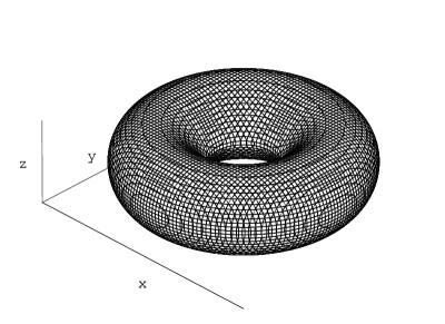
Figure 1: Equidensity surface for the quantized deuteron

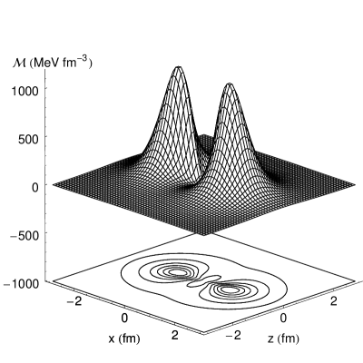
Figure 2: Mass density distribution of the quantized deuteron

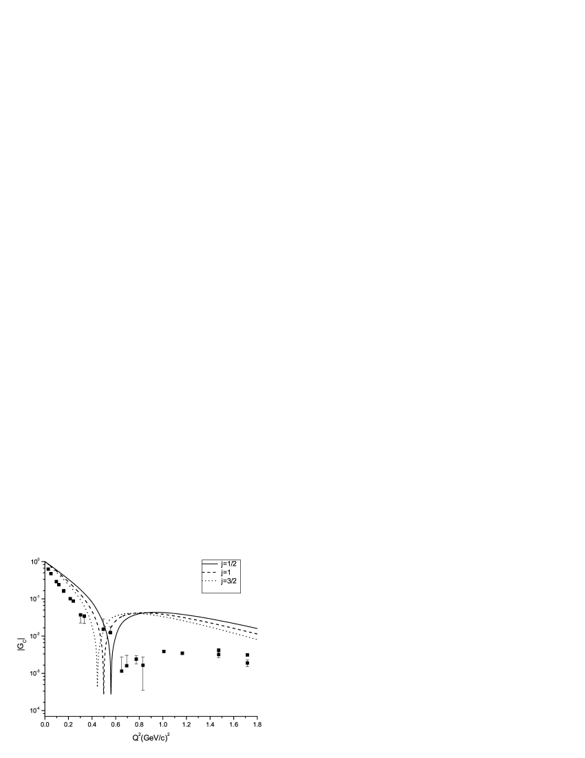
Figure 3: Electric form factor of the quantized deuteron solution. The experimental data are from [16]

References

• [1] T. H. R. Skyrme, Proc. Roy. Soc. A260, 27 (1961).
• [2] R.A. Battye and P.M. Sutcliffe, Phys. Rev. Lett. 79, 363 (1997).
• [3] N.S. Manton, Phys. Lett. B 192, 177 (1987); J.J.M. Verbaarschot, Phys. Lett. B 195, 235 (1987); V.B. Kopeliovich and B.E. Stern, JETP Lett. 45, 203 (1987).
• [4] I. Sick, Prog. Part. Nucl. Phys. 47, 245 (2001).
• [5] C.J. Houghton, N.S. Manton and P.M. Sutcliffe, Nucl. Phys. B 510, 507 (1998).
• [6] G.S. Adkins, C.R. Nappi and E. Witten, Nucl. Phys. B 228, 552(1983)
• [7] E. Braaten, L. Carson, Phys. Rev. D 38, 3525 (1988).
• [8] K. Fujii, A. Kobushkin, K. Sato and N. Toyota, Phys. Rev. Lett. 58, 651 (1987); Phys. Rev. D 35, 1896 (1987).
• [9] A. Acus, E. Norvaišas and D.O. Riska, Phys. Rev. C 57, 2597 (1998).
• [10] E. Norvaišas and D.O. Riska, Physica Scripta 50, 634 (1994)
• [11] A. Acus, E. Norvaišas and D.O. Riska, Nucl. Phys. A 614, 361(1997).
• [12] T. Krupovnickas and E. Norvaišas, D.O. Riska, Lithuanian J. Phys. 41, 13 (2001).
• [13] R. A. Leese, N. S. Manton and B. J. Schroers, Nucl. Phys. B442, 228 (1995)
• [14] J.L. Forest et.al., Phys. Rev. C 54, 646 (1996).
• [15] E.M. Nyman and D.O. Riska, Nucl. Phys. A 468, 473 (1987).
• [16] D. Abbott et al., Eur. Phys. J. A 7, 421 (2000).
Refer to caption