Superdeformed bands in neutron-rich Sulfur isotopes suggested by cranked Skyrme-Hartree-Fock calculations

Abstract

On the basis of the cranked Skyrme-Hartree-Fock calculations in the three-dimensional coordinate-mesh representation, we suggest that, in addition to the well-known candidate ³²S, the neutron-rich nucleus ³⁶S and the drip-line nuclei, ⁴⁸S and ⁵⁰S, are also good candidates for finding superdeformed rotational bands in Sulfur isotopes. Calculated density distributions for the superdeformed states in ⁴⁸S and ⁵⁰S exhibit superdeformed neutron skins.

PACS: 21.60-n; 21.60.Jz; 27.30.+t

Keywords: Cranked Skyrme-Hartree-Fock method; Superdeformation; Neutron-rich nuclei; High-spin state; Sulfur isotopes

1 Introduction

Recently, superdeformed (SD) rotational bands have been discovered in ³⁶Ar, ⁴⁰Ca and ⁴⁴Ti [1, 2, 3, 4, 5, 6]. One of the interesting new features of them is that they are built on excited $0^{+}$ states and observed up to high spin, in contrast to the SD bands in heavier mass regions where low-spin portions of them are unknown in almost all cases [7, 8, 9, 10, 11]. These excited $0^{+}$ states may be associated with multiparticle-multihole excitations from the spherical closed shells, so that we can hope to learn from such data detailed relationships between spherical shell model and SD configurations. For the mass $A=$30-50 region, although existence of a SD band in ³²S with the SD magic number $N=Z=16$ has been expected for a long time [12], it has not yet been observed and remains as a great challenge [13, 14, 15, 16, 17].

In this paper, as a continuation of the systematic theoretical search [14, 18] for SD bands in the mass $A=$30-50 region by means of the cranked Skyrme-Hartree-Fock (SHF) method[19], we would like to suggest that, in addition to ³²S, the neutron-rich nucleus ³⁶S and the nuclei, ⁴⁸S and ⁵⁰S, which are situated close to the neutron-drip line[20, 21], are also good candidates for finding SD rotational bands in Sulfur isotopes. The appearance of the SD band in ³⁶S is suggested in connection with the SD shell structure at $N=20$ characterizing the observed SD band in ⁴⁰Ca. The drip-line nuclei, ⁴⁸S and ⁵⁰S, are expected to constitute a new “SD doubly closed” region associated with the SD magic numbers, $Z=16$ for protons and $N\simeq 32$ for neutrons. An interesting theoretical subject for the SD bands in nuclei near the neutron drip line is to understand deformation properties of neutron skins. The calculated density distributions indeed exhibit superdeformed neutron skins.

The calculation has been carried out with the use of the three-dimensional (3D), Cartesian coordinate-mesh representation without imposing any symmetry restriction[14, 18]. In parallel, we also carry out the standard calculations [22, 23, 24, 25] imposing reflection symmetries. By comparing the symmetry restricted and unrestricted calculations, we can examine the stability of the SD solutions of the SHF equations against reflection-asymmetric deformations. In this way, we have found several cases where the SD minima obtained in the symmetry-restricted calculations are in fact unstable with respect to the reflection-asymmetric deformations. In general, the SD states are rather soft against reflection-asymmetric deformations, so that we need careful study about the stabilities of them against various kinds of deformation breaking the reflection symmetries.

After a brief account of the cranked SHF calculational procedure in Section 2, we present and discuss results of the calculation in Section 3, and give conclusions in Section 4. We shall present deformation energy curves for Sulfur isotopes from ³²S to ⁵⁰S, and focus our attention on properties of rotational bands built on the SD $0^{+}$ states, stabilities of the SD local minima against the reflection-asymmetric deformations, and density distributions of the SD states.

A preliminary version of this work was reported in [26].

2 Cranked SHF calculation

Since the cranked SHF method in the 3D coordinate-mesh representation is well known[22, 23, 24, 25], we here give only a minimum description about the computational procedure actually adopted. For a recent comprehensive review on selfconsistent mean-field models for nuclear structure, see Ref. [19]. The cranked SHF equation for a system uniformly rotating about the $x$-axis is given by

$$\delta<H-\omega_{\rm rot}\hat{J}_{x}>=0,$$ (1)

where $H$, $\omega_{\rm rot}$ and $\hat{J}_{x}$ mean the Hamiltonian with the Skyrme interaction, the rotational frequency and the $x$-component of angular momentum, respectively, and the bracket denotes the expectation value with respect to a Slater determinantal state. We solve the cranked SHF equation by means of the imaginary-time evolution technique[22] in the 3D Cartesian-mesh representation. The algorithm of numerical calculation is the standard one [22, 23, 24, 25], except that we allow for both reflection- and axial-symmetry breakings. In this case, it is important to accurately fulfill the center-of-mass and principal-axis conditions. This is done by means of the constrained HF procedure[27]. We solved these equations inside the sphere with radius $R$=10 fm and mesh size $h$=1 fm, starting with various initial configurations. The accuracy for evaluating deformation energies with this mesh size was carefully checked by Tajima[25] and was found to be quite satisfactory. When we make a detailed analysis of density distributions, however, we use a smaller mesh size of $h=\frac{1}{3}$ fm. In addition to the symmetry-unrestricted cranked SHF calculation, we also carry out symmetry-restricted calculations imposing reflection symmetries about the $(x,y)$-, $(y,z)$- and $(z,x)$-planes. Below we call these symmetry-unrestricted and -restricted cranked SHF versions “unrestricted” and “restricted” ones, respectively.

Solutions of the cranked SHF equation give local minima in the deformation energy surface. In order to explore the deformation energy surface around these minima and draw deformation energy curves as functions of deformation parameters, we carry out the constrained HF procedure with relevant constraining operators[27]. For the Skyrme interaction, we adopt the widely used three versions; SIII [28], SkM^∗[29] and SLy4 [30].

3 Results of calculation

3.1 Deformation energy curves

Figure 1 shows deformation energy curves for Sulfur isotopes from ³²S to ⁵⁰S obtained with the use of the SIII interaction. Solid lines with and without filled circles represent the results obtained by the unrestricted and restricted versions, respectively. The result of calculation indicates that the SD minima (with the quadrupole deformation parameter $\beta_{2}\approx 0.6$) appear in the neutron-rich nucleus ³⁶S and the drip-line nuclei, ⁴⁸S and ⁵⁰S, in addition to the well-known case of ³²S. As seen in Figs. 2 and 3, similar results are obtained for the SkM^∗ and SLy4 interactions, except that the SD states in ⁴⁸S is unstable against the reflection-asymmetric deformation for the SLy4 interaction (see subsection 3.3).

As discussed in Refs.[14, 15, 16, 17, 18], the SD local minimum in ³²S corresponds to the doubly closed shell configuration with respect to the SD magic number $Z=N=16$ and involves two protons and two neutrons in the down-sloping single-particle levels originating from the $f_{7/2}$ shell. The SD local minimum in ³⁶S results from the coherent combination of the SD magic number, $Z=16$, and the neutron shell effects occurring at large deformation for $N=20$. The latter shell effect has been confirmed recently by the discovery of the SD rotation band in ⁴⁰Ca [4, 5]. The SD shell gap at $N=20$ is associated with the 4p-4h excitation from below the $N=20$ spherical closed shell to the $f_{7/2}$ shell. Focusing our attention on the occupation numbers of such high-$j$ shells and distinguishing protons($\pi$) and neutrons($\nu$), these SD configurations in ³²S and ³⁶S are denoted in Figs. 1-3 as $f_{\pi}^{2}f_{\nu}^{2}$ and $f_{\pi}^{2}f_{\nu}^{4}$, respectively.

The SD local minima in the drip-line nuclei, ⁴⁸S and ⁵⁰S, result from the coherent combination of the proton SD shell effect and the neutron shell effects occurring at superdeformation for $N=$32-34. The neutron configurations in these SD states are similar to those in the known SD bands in ⁶⁰Zn and ⁶²Zn associated with the SD magic numbers $N=$30-32[31, 32]. We find that the SD shell effect is strong also for $N=34$ in the Sulfur isotopes under consideration, while the SD local minimum in ⁴⁶S with $N=30$ is unstable against the reflection-asymmetric deformation (see subsection 3.3). In the drip-line nuclei ⁴⁸S and ⁵⁰S, the $f_{7/2}$ shell is fully occupied even in the spherical limit and the SD configurations involve neutron excitations from the $fp$-shell to the $g_{9/2}$ shell. As before, focusing our attention on the occupation numbers of the high-$j$ shells, let us use the notation $f_{\pi}^{n_{1}}g_{\nu}^{n_{2}}$ for a configuration in which single-particle levels originating from the $f_{7/2}$ and $g_{9/2}$ shell are occupied by $n_{1}$ protons and $n_{2}$ neutrons, respectively. With such notations, the SD local minima in ⁴⁸S and ⁵⁰S correspond to the $f_{\pi}^{2}g_{\nu}^{2}$, and $f_{\pi}^{2}g_{\nu}^{4}$ configurations, respectively.

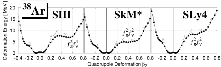
Figure 4: The same as Fig.1 but for ³⁸Ar and for the SIII, SkM^∗ and SLy4 interactions.

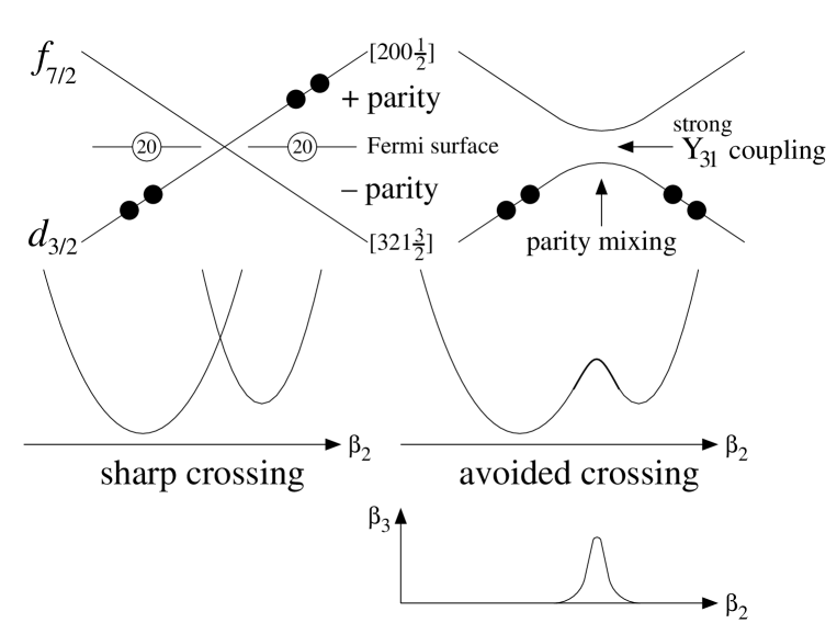
Figure 5: Schematic illustration of configuration-mixing mechanism through the octupole components of the mean field. When the reflection symmetry is imposed, the positive- and negative-parity single-particle levels sharply cross, and the two configurations (having different number of particles in the $f_{7/2}$ shell) do not mix within the mean-field approximation (left-hand side). In contrast, when such symmetry restriction is removed, smooth crossover between the two configurations is possible via mixing of the positive- and negative-parity levels (right-hand side). Octupole deformation $\beta_{3}$ of the mean field rises in the crossing region. In this figure, the crossing between the two levels with the asymptotic quantum numbers $[321\frac{3}{2}]$ and $[200\frac{1}{2}]$ is illustrated as an example. The two levels satisfy the selection rule, $\Delta n_{3}=2$ and $\Delta\Lambda=1$, for the matrix elements of the non-axial octupole operator $r^{3}Y_{31}$, so that the mixing between them takes place mainly through the $r^{3}Y_{31}$ component of the mean field.

The appearance of the SD minimum in ³⁶S suggests that we can expect a SD band associated with the same neutron configuration to appear also in the $N=20$ isotone, ³⁸Ar, situated between ³⁶S and ⁴⁰Ca. We examined this point and the result is shown in Fig. 4. We find that the two local minima associated with the configurations $f_{\pi}^{2}f_{\nu}^{2}$ and $f_{\pi}^{2}f_{\nu}^{4}$ compete in energy and their relative energy differs for different versions of the Skyrme interaction: As clearly seen in the deformation-energy curves obtained by the symmetry-restricted calculations, the former with smaller $\beta_{2}$ is slightly lower for SkM^∗ and SLy4 while the latter with larger $\beta_{2}$ is slightly lower for SIII. Counting both protons and neutrons, these local minima respectively correspond to the 4p-6h and 6p-8h configurations with respect to the spherical doubly closed shell of ⁴⁰Ca. As we discussed in the previous papers[18, 26], the two configurations can mix each other in the crossing region through the reflection-symmetry breaking components in the mean field. Specifically, around the crossing point between the down-sloping $[321\frac{3}{2}]$ level (coming from the $f_{7/2}$ shell) and the up-sloping $[200\frac{1}{2}]$ level (coming from the $d_{3/2}$ shell below the $N=20$ spherical magic number), the $r^{3}Y_{31}$-type non-axial octupole deformation is generated, and they mix each other through this component of the mean field (see Fig. 5). Note that the matrix element of the operator $r^{3}Y_{31}$ between the two levels satisfies the selection rules, $\Delta n_{3}=2$ and $\Delta\Lambda=1$, for the asymptotic quantum numbers $n_{3}$ and $\Lambda$. As a result of this mixing, the deformation-energy curve becomes rather flat in the symmetry-unrestricted calculation. Recently, the SD band corresponding to the 4p-6h configuration was found in experiment[33]. The data suggest significant competition between different configurations, which requires further analysis of shape fluctuation dynamics by going beyond the static mean-field approximation.

3.2 SD rotational bands

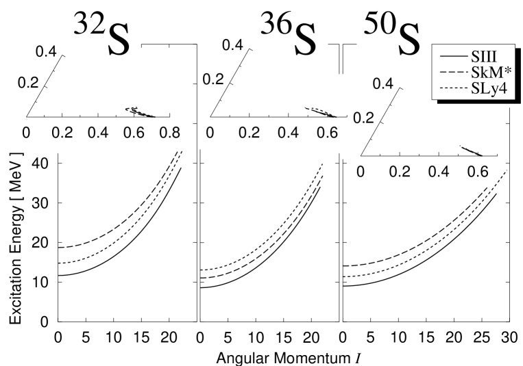
Figure 6: Plot of the excitation energies versus angular-momentum for the SD rotational bands in ³²S, ³⁶S, and ⁵⁰S calculated by means of the cranked SHF method. Results obtained with the use of the SIII, SkM^∗, and SLy4 interactions are plotted by solid, dashed, and dotted curves, respectively. Their shape evolutions as functions of angular momentum $I$ in the $(\beta_{2},\gamma)$ plane are displayed in the upper portions. The $\beta_{2}$ values decrease with increasing $I$.

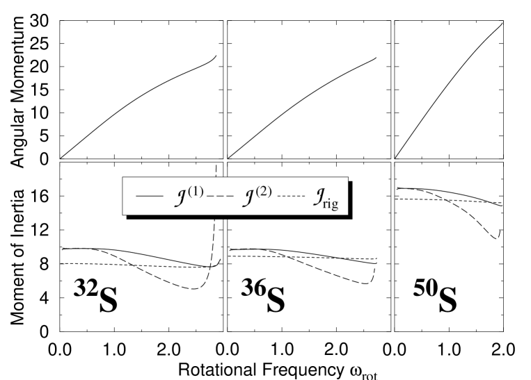
Figure 7: The angular momenta $I$ and the moments of inertia ${\cal J}$ are plotted as functions of rotational frequency $\omega_{\rm rot}$ for the SD rotational bands in ³²S, ³⁶S, and ⁵⁰S. The SLy4 interaction is used. Values of the kinematical and dynamical moments of inertia, ${\cal J}^{(1)}=I/\omega_{\rm rot}$ and ${\cal J}^{(2)}=dI/d\omega_{\rm rot}$, are plotted in unit of $\hbar^{2}$/MeV by solid and dashed curves, respectively. For reference, the rigid-body moments of inertia ${\cal J}_{\rm rig}=m\int\rho({\mbox{\boldmath$r$}})(y^{2}+z^{2})d{\mbox{\boldmath$r$}}$ evaluated with the calculated density $\rho({\mbox{\boldmath$r$}})$ are also indicated.

Let us focus our attention on the SD local minima shown in Figs. 1-3, and investigate properties of the rotational bands built on them. Excitation energies of these SD rotational bands are plotted in Fig. 6 as functions of angular momentum. These rotational bands are calculated by cranking each SHF solution (the SD local minima in Figs. 1-3) and following the same configuration with increasing value of $\omega_{\rm rot}$ until the point where we cannot clearly identify the continuation of the same configuration any more. Thus, the highest values of angular momentum in this figure does not necessarily indicate the band-termination points but merely suggest that drastic changes in their microscopic structure take place around there. Different slopes with respect to the angular momentum between ³⁶S and ⁵⁰S can be easily understood in terms of the well known scaling factor $A^{5/3}$ for the rigid-body moment of inertia. This point can be confirmed in Fig. 7 which displays the angular momentum $I$, the kinematical and dynamical moments of inertia, ${\cal J}^{(1)}=I/\omega_{\rm rot}$ and ${\cal J}^{(2)}=dI/d\omega_{\rm rot}$, and the rigid-body moments of inertia ${\cal J}_{\rm rig}=m\int\rho({\mbox{\boldmath$r$}})(y^{2}+z^{2})d{\mbox{\boldmath$r$}}$ as functions of the rotational frequency $\omega_{\rm rot}$. We see that the calculated moments of inertia are slightly larger than the rigid-body values at $\omega_{\rm rot}=0$, and smoothly decrease as $\omega_{\rm rot}$ increases until $\omega_{\rm rot}\approx$2.5 and 1.8 MeV$/\hbar$ for ^32,36S and ⁵⁰S, respectively. The result calculated with the SLy4 interaction is shown here, but we obtained similar results also with the SIII and SkM^∗ interactions.

Calculated quadrupole deformation parameters $(\beta_{2},\gamma)$ are displayed in the upper portion of Fig. 6. We see that the $\beta_{2}$ values slowly decrease while the axial-asymmetry parameters $\gamma$ gradually increase with increasing angular momentum for all cases of ³²S, ³⁶S and ⁵⁰S. The variations are rather mild in the range of angular momentum shown in this figure. Single-particle energy diagrams (Routhians) for these SD bands are displayed in Fig. 8 as functions of the rotational frequency $\omega_{\rm rot}$. This figure indicates that level crossings take place in ³⁶S and ⁵⁰S if we further increase the angular momentum.

3.3 Stabilities of the SD states against reflection-asymmetric deformations

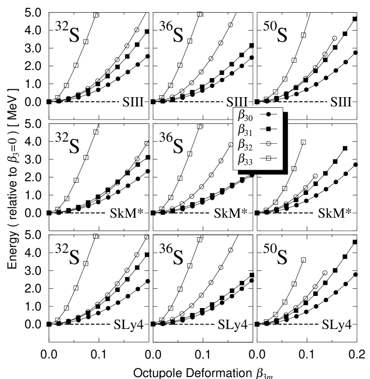
Figure 9: Deformation energy curves (measured from energies at $\beta_{3}=0$) as functions of the octupole deformation parameters $\beta_{3m}(m=0,1,2,3)$, calculated for ³²S, ³⁶S, and ⁵⁰S, by means of the constrained HF procedure with the use of the SIII, SkM^∗ and SLy4 interactions. The quadrupole deformation parameters are fixed at the equilibrium value of $\beta_{2}$ in each nucleus and $\gamma=0$. One of the $\beta_{3m}(m=0,1,2,3)$ is varied while the other $\beta_{3m}$’s are fixed to zero. The deformation parameters $\beta_{3}$ and $\beta_{3m}$ are defined in terms of the expectation values of the octupole operators (see Ref.[18] for their explicit expressions).

Let us examine stabilities of the SD local minimum against both the axially symmetric and asymmetric octupole deformation ($Y_{30},Y_{31},Y_{32},Y_{33}$). Figure 9 presents deformation energy curves as functions of the octupole deformation parameters $\beta_{3m}(m=0,1,2,3)$ for fixed quadrupole deformation parameters (the equilibrium value of $\beta_{2}$ at the SD minimum in each nucleus and $\gamma=0$). The computation was carried out by means of the constrained HF procedure with the use of the SIII, SkM^∗, and SLy4 interactions. The result of calculation clearly indicates that the SD states in ³²S, ³⁶S and ⁵⁰S are stable against the octupole deformations and that they are softer for $\beta_{3m}$ with lower values of $m$ (i.e., for $\beta_{30}$ and $\beta_{31}$), irrespective of the Skyrme interactions used. We obtaind a similar result also for ⁴⁸S (but omitted in this figure).

Although the SD minima in ³²S, ³⁶S and ⁵⁰S are stable with respect to $\beta_{3m}(m=0,1,2,3)$, we found several cases where the SD minima obtained in the symmetry-restricted calculations become unstable when we allow for reflection-asymmetric deformations of a more general type. As a first example, let us discuss the SD minimum in ⁴⁶S which appears in the restricted calculation (see Figs. 1-3). In this case, the coupling between the down-sloping $[330\frac{1}{2}]$ level (associated with the $f_{7/2}$ shell) and the up-sloping $[202\frac{5}{2}]$ level (stemming from the $d_{5/2}$ shell) takes place in the proton configuration, when we allow for the breaking of both the axial and reflection symmetries. Thus, the SD configuration $f_{\pi}^{2}g_{\nu}^{2}$ mixes with the $g_{\nu}^{2}$ configuration (which lacks the proton excitation to the $f_{7/2}$ shell and has a smaller equilibrium value of $\beta_{2}$). As a consequence of this mixing, the barrier between the two configurations disappears and the SD minimum becomes unstable in the unrestricted calculations (see Figs. 1-3). Note that the difference $\Delta n_{3}$ in the asymptotic quantum number $n_{3}$ between the two single-particle levels, $[330\frac{1}{2}]$ and $[202\frac{5}{2}]$, is three, so that they cannot be mixed by the octupole operator $r^{3}Y_{32}$ which transfers the asymptotic quantum numbers $n_{3}$ and $\Lambda$ by $\Delta n_{3}=1$ and $\Delta\Lambda=2$. Thus, this mixing may be associated with the reflection-asymmetric deformation of a more higher order like $r^{5}Y_{52}$.

As a second example, we take up the SD minimum in ⁴⁸S. In this case, two configurations, $f_{\pi}^{2}g_{\nu}^{2}$ and $f_{\pi}^{2}g_{\nu}^{4}$ compete in energy and their relative energy differs for different versions of the Skyrme interaction (see Figs. 1-3). When we allow for the breaking of both the axial and reflection symmetries, the coupling between the down-sloping $[431\frac{3}{2}]$ level (associated with the $g_{9/2}$ shell) and the $[310\frac{1}{2}]$ level in the $fp$ shell takes place in the neutron configuration, so that they mix each other. Note that the $[431\frac{3}{2}]$ and $[310\frac{1}{2}]$ levels satisfy the selection rules, $\Delta n_{3}=2$ and $\Delta\Lambda=1$, for the matrix elements of the octupole operator $r^{3}Y_{31}$. In the calculation with the SLy4 interaction, since the former configuration with smaller $\beta_{2}$ is situated slightly lower in energy than the latter, the barrier between the two configurations disappears as a result of this mixing. This mixing effect in conjunction with that mentioned above for the $f_{\pi}^{2}g_{\nu}^{2}$ configuration in ⁴⁶S deteriorates the SD minimum for the SLy4 case.

The above examples indicate detailed microscopic mechanisms within the mean-field theory how the stability of the SD local minimum is determined by relative energies between the neighboring configurations and their mixing properties.

3.4 Density distributions

Figure 10 displays the neutron and proton density profiles for the SD states in ³²S, ³⁶S and ⁵⁰S calculated with the use of the SLy4 interaction. We obtained similar results also for SIII and SkM^∗. In this figure, equi-density lines with 50% and 1% of the central density in the $(x,y)$- and $(y,z)$-planes are drawn for the SD bands at $I=0$ and at high spins. We can clearly see that superdeformed neutron skin appears in ⁵⁰S which is situated close to the neutron drip line. The root-mean-square values, $\sqrt{\langle x^{2}\rangle},\sqrt{\langle y^{2}\rangle},\sqrt{\langle z^{2}\rangle}$ and $R_{\rm rms}=\sqrt{\langle\mbox{\boldmath$r$}^{2}\rangle}$, of these density distributions are listed in Table 1. To indicate the deformation properties of the neutron skin in ⁵⁰S, calculated values for protons and neutrons are separately listed together with their sums and differences. We obtained density distributions similar to those for ⁵⁰S also for the SD state in ⁴⁸S. A similar result of theoretical calculation exhibiting the superdeformed neutron skin was previously reported in Ref.[34] for the SD state in the very neutron-rich nucleus ${}_{~{}66}^{208}$Dy₁₄₂.

4 Conclusions

On the basis of the cranked SHF calculations in the 3D coordinate-mesh representation, we have suggested that, in addition to the well-known candidate ³²S, the neutron-rich ³⁶S and the the drip-line nuclei, ⁴⁸S and ⁵⁰S, are also good candidates for finding SD rotational bands in Sulfur isotopes. Calculated density distributions for the SD states in ⁴⁸S and ⁵⁰S, which are situated close to the neutron-drip line, exhibit superdeformed neutron skins.

Table 1

Root-mean-square values, $\sqrt{\langle x^{2}\rangle},\sqrt{\langle y^{2}\rangle},\sqrt{\langle z^{2}\rangle}$ and $R_{\rm rms}=\sqrt{\langle\mbox{\boldmath$r$}^{2}\rangle}$, of the density distributions at $I=0$ (second column) and at $I=20,22,28$ (third column) of the SD band in ³²S, ³⁶S and ⁵⁰S, calculated with the use of the SLy4 interaction. Neutron and proton contributions are separately listed together with their sums (total) and differences (diff.).

32S	$I=0$				$I\sim 20$
	$\sqrt{\langle x^{2}\rangle}$	$\sqrt{\langle y^{2}\rangle}$	$\sqrt{\langle z^{2}\rangle}$	$R_{\mathrm{rms}}$	$\sqrt{\langle x^{2}\rangle}$	$\sqrt{\langle y^{2}\rangle}$	$\sqrt{\langle z^{2}\rangle}$	$R_{\mathrm{rms}}$
total	1.53	1.53	2.85	3.57	1.53	1.67	2.67	3.50
neutrons	1.52	1.52	2.83	3.55	1.52	1.66	2.65	3.48
protons	1.54	1.54	2.86	3.60	1.54	1.68	2.68	3.52
diff.	-0.02	-0.02	-0.04	-0.04	-0.02	-0.02	-0.04	-0.05
36S	$I=0$				$I\sim 22$
	$\sqrt{\langle x^{2}\rangle}$	$\sqrt{\langle y^{2}\rangle}$	$\sqrt{\langle z^{2}\rangle}$	$R_{\mathrm{rms}}$	$\sqrt{\langle x^{2}\rangle}$	$\sqrt{\langle y^{2}\rangle}$	$\sqrt{\langle z^{2}\rangle}$	$R_{\mathrm{rms}}$
total	1.59	1.59	2.78	3.58	1.61	1.73	2.63	3.53
neutrons	1.62	1.62	2.78	3.60	1.64	1.75	2.64	3.57
protons	1.55	1.55	2.78	3.54	1.57	1.69	2.61	3.48
diff.	0.07	0.07	0.00	0.06	0.08	0.06	0.03	0.09
50S	$I=0$				$I\sim 28$
	$\sqrt{\langle x^{2}\rangle}$	$\sqrt{\langle y^{2}\rangle}$	$\sqrt{\langle z^{2}\rangle}$	$R_{\mathrm{rms}}$	$\sqrt{\langle x^{2}\rangle}$	$\sqrt{\langle y^{2}\rangle}$	$\sqrt{\langle z^{2}\rangle}$	$R_{\mathrm{rms}}$
total	1.81	1.81	3.11	4.03	1.82	1.96	2.95	3.98
neutrons	1.90	1.90	3.17	4.16	1.91	2.05	3.02	4.12
protons	1.62	1.62	2.96	3.75	1.63	1.75	2.79	3.67
diff.	0.28	0.28	0.20	0.41	0.28	0.31	0.23	0.45

Figure 1: Deformation energy curves for Sulfur isotopes from ³²S to ⁵⁰S calculated at $I=0$ as functions of the quadrupole deformation $\beta_{2}$ by means of the constrained SHF procedure with the SIII interaction. The deformation parameter is defined as $\beta_{2}=\frac{4\pi}{5}~{}\langle\sum_{i=1}^{A}r_{i}^{2}Y_{20}(\theta_{i},\phi_{i})\rangle/\langle\sum_{i=1}^{A}\mbox{\boldmath$r$}_{i}^{2}\rangle.$ The axial-asymmetry parameter $\gamma$ is constrained to be zero. Solid curves with and without filled circles represent the results obtained by the unrestricted and restricted versions, respectively. The notation $f_{\pi}^{n_{1}}f_{\nu}^{n_{2}}$ indicates a configuration in which single-particle levels originating from the $f_{7/2}$ shell are occupied by $n_{1}$ protons and $n_{2}$ neutrons. Likewise, $f_{\pi}^{n_{1}}g_{\nu}^{n_{2}}$ indicates that levels from the $f_{7/2}$ shell are occupied by $n_{1}$ protons and those from the $g_{9/2}$ shell by $n_{2}$ neutrons.

Figure 2: The same as Fig.1 but for the SkM^∗ interaction.

Figure 3: The same as Fig.1 but for the SLy4 interaction.

Figure 8: Single-particle energy diagrams (Routhians) for the SD bands in ³²S, ³⁶S, and ⁵⁰S, plotted as functions of rotational frequency $\omega_{\rm rot}$. The left(right)-hand side displays those for protons(neutrons). The levels associated with the $g_{9/2}$ and $f_{7/2}$ shells are drawn by thick-solid and thick-dashed lines, respectively. Other occupied levels associated with the $sd$ and $fp$ shells are drawn by thin-solid and thin-dashed lines, respectively. Unoccupied levels are drawn by thin-dotted lines. Numbers indicate the Fermi surfaces and total numbers of single-particle states below them. The result calculated with SLy4 is shown here, but we obtained similar results also with SIII and SkM^∗.

Figure 10: Left-hand side: Density distributions in the $(y,x)$- and $(z,x)$- planes of the SD band at $I=0$ in ³²S, ³⁶S, and ⁵⁰S, calculated with the use of the SLy4 interaction. Neutron (proton) equi-density lines with 50% and 1% of the central density are shown by dashed (solid) lines (the inner and outer lines correspond to the 50% and 1% lines, respectively). Right-hand side: Same as the left-hand side but for $I=20,22,28$ for ³²S, ³⁶S, and ⁵⁰S, respectively.

References

- [1] C.E. Svenson et al., Phys. Rev. Lett. 85 (2000) 2693.
- [2] C.E. Svenson et al., Phys. Rev. C 63 (2001) 061301(R).
- [3] C.E. Svenson et al., Nucl. Phys. A 682 (2001) 1c.
- [4] E. Ideguchi et al., Phys. Rev. Lett. 87 (2001), 222501.
- [5] C.J. Chiara et al., Phys. Rev. C 67 (2003), 041303(R).
- [6] C.D. O’Leary, M.A. Bentley, B.A. Brown, D.E. Appelbe, R.A. Bark, D.M. Cullen, S. Ertürk, A. Maj and A.C. Merchant, Phys. Rev. C 61 (2000) 064314.
- [7] P.J. Nolan and P.J. Twin, Annu. Rev. Nucl. Part. Sci. 38 (1988) 533.
- [8] S. Åberg, H. Flocard and W. Nazarewicz, Annu. Rev. Nucl. Part. Sci. 40 (1990) 439.
- [9] R.V.F. Janssens and T.L. Khoo, Annu. Rev. Nucl. Part. Sci. 41 (1991) 321.
- [10] C. Baktash, B. Haas and W. Nazaerewicz, Annu. Rev. Nucl. Part. Sci. 45 (1995) 485.
- [11] C. Baktash, Prog. Part. Nucl. Phys. 38 (1997) 291.
- [12] I. Ragnarsson, S.G. Nilsson and R.K. Sheline, Phys. Rep. 45 (1978) 1.
- [13] J. Dobaczewski, Proc. Int. Conf. on Nuclear Structure ’98 (AIP conference proceedings 481), ed. C. Baktash, p. 315.
- [14] M. Yamagami and K. Matsuyanagi, Nucl. Phys. A 672 (2000) 123.
- [15] H. Molique, J. Dobaczewski, J. Dudek, Phys. Rev. C 61 (2000) 044304.
- [16] R.R. Rodriguez-Guzmán, J.L. Egido and L.M. Robeldo, Phys. Rev. C 62 (2000) 054308.
- [17] T. Tanaka, R.G. Nazmitdinov and K. Iwasawa, Phys. Rev. C 63 (2001) 034309.
- [18] T. Inakura, S. Mizutori, M. Yamagami and K. Matsuyanagi, Nucl. Phys. A 710 (2002) 261.
- [19] M. Bender, P.-H. Heenen and P-G. Reinhard, Rev. Mod. Phys. 75 (2003) 121.
- [20] T.R. Werner, J.A. Sheikh, W. Nazarewicz, M.R. Strayer, A.S. Umar and M. Misu, Phys. Lett. B 333 (1994) 303.
- [21] T.R. Werner, J.A. Sheikh, M. Misu, W. Nazarewicz, J. Rikovska, K. Heeger, A.S. Umar and M.R. Strayer, Nucl. Phys. A 597 (1996) 327.
- [22] K.T.R. Davies, H. Flocard, S.J. Krieger and M.S. Weiss, Nucl. Phys. A 342 (1980) 111.
- [23] P. Bonche, H. Flocard, P.H. Heenen, S.J. Krieger and M.S. Weiss, Nucl. Phys. A 443 (1985) 39.
- [24] P. Bonche, H. Flocard, P.H. Heenen, Nucl. Phys. A 467 (1987) 115.
- [25] N. Tajima, Prog. Theor. Phys. Supple. No. 142 (2001) 265.
- [26] T. Inakura, M. Yamagami, K. Matsuyanagi and S. Mizutori, Proc. Int. Symp. “Frontiers of Collective Motions,” Aizu-Wakamatsu, Japan, Nov. 6-9, 2002, in press.
- [27] H. Flocard, P. Quentin, A.K. Kerman and D. Vautherin, Nucl. Phys. A 203 (1973) 433.
- [28] M. Beiner, H. Flocard, Nguyen van Giai and P. Quentin, Nucl. Phys. A 238 (1975) 29.
- [29] J. Bartel, P. Quentin, M. Brack, C. Guet and H.-B. Håkansson, Nucl. Phys. A 386 (1982) 79.
- [30] E. Chabanat, P. Bonche, P. Haensel, J. Meyer and F. Schaeffer, Nucl. Phys. A 635 (1998) 231.
- [31] C.E. Svensson et al., Phys. Rev. Lett. 82 (1999) 3400.
- [32] C.E. Svensson et al., Phys. Rev. Lett. 79 (1997) 1233.
- [33] D. Rudolph et al., Phys. Rev. C 65 (2002) 034305.
- [34] I. Hamamoto and X.Z. Zhang, Phys. Rev. C 52 (1995) R2326.