Antiprotonic Potentials from Global Fits to the PS209 Data

Abstract

The experimental results for strong interaction effects in antiprotonic atoms by the PS209 collaboration consist of high quality data for several sequences of isotopes along the periodic table. Global analysis of these data in terms of a $\bar{p}$-nucleus optical potential achieves good description of the data using a $s$-wave finite-range $\bar{p}N$ interaction. Equally good fits are also obtained with a poorly-defined zero-range potential containing a $p$-wave term.

,

1 Introduction

In earlier publications [1, 2] most of the then available data on strong interaction effects in antiprotonic atoms have been used in ‘global’ analyses in terms of a $\bar{p}$-nucleus optical potential. The simplest form of the potential is

$$2\mu V_{{\rm opt}}(r)=-4\pi(1+\frac{\mu}{M}\frac{A-1}{A})[b_{0}(\rho_{n}+\rho_{p})+b_{1}(\rho_{n}-\rho_{p})]~{}~{},$$ (1)

where $\mu$ is the $\bar{p}$-nucleus reduced mass, $\rho_{n}$ and $\rho_{p}$ are the neutron and proton density distributions normalized to the number of neutrons $N$ and number of protons $Z$, respectively, $A=N+Z$ and $M$ is the mass of the nucleon. In the zero-range ‘$t\rho$’ approach the parameters $b_{0}$ and $b_{1}$ are minus the $\bar{p}$-nucleon isoscalar and isovector scattering lengths, respectively, otherwise these parameters may be regarded as ‘effective’. The fits of Ref. [1] were based on 48 data points which included only two pairs of isotopes. As a typical result we quote Re$b_{0}=2.51\pm 0.24$ fm, Im$b_{0}=3.46\pm 0.27$ fm, leading to $\chi^{2}$/N, the $\chi^{2}$ per point, of 1.5, which represents a very good fit to the data. Additional terms had also been cosidered in [1] such as a $p$-wave term, which led to $\chi^{2}$/N in the range of 1.2 to 1.4. Such a reduction in $\chi^{2}$ is, however, not statistically significant in these circumstances. Consequently only the above zero-range $b_{0}$ version has since been used in several analyses of experimental results.

The recent publication of results for strong interaction effects in antiprotonic atoms by the PS209 collaboration [3] changed the experimental situation dramatically by providing high quality data for several sequences of isotopes along the periodic table. Such data hold promise to pin-point isospin effects in the potential and/or explicit surface effects such as the existence of a $p$-wave term in the potential. This is the scope of the present work which is based on data for five isotopes of Ca, four isotopes each of Fe and of Ni, two isotopes each of Zr and of Cd, four isotopes of Sn, five isotopes of Te and the isotope ²⁰⁸Pb, all from results of the PS209 collaboration [3]. Note that the results for Cd, Sn and Te isotopes have been revised very recently to include effects of E2 resonance [4, 5]. In order to expand the range of the data further we have included also earlier results for ^16,18O (see [1] for references to the original experiments.) In section 2 we discuss the choice of nuclear density distributions $\rho_{n}$ and $\rho_{p}$, which form an essential ingredient of the optical potential Eq. (1). Section 3 summarizes the results and presents a ‘recommended’ set of parameters which best describes the data.

2 Density distributions

In choosing the nuclear density distributions for use in the analysis of strong interaction effects in antiprotonic atoms, one is faced with the fact that due to the strength of the $\bar{p}$-nucleus interaction and the dominant role played by the imaginary potential, strong interaction effects reflect the interaction with the extreme outer regions of the nucleus where the density is well below 10% of the central density. It is therefore not very reliable to infer from these data quantities which relate to the bulk of the density such as root mean square (rms) radii. In what follows we therefore rely also on information from pionic atoms [6] when choosing the densities, bacause pionic atoms are sensitive to the region where the density is 50% or more of the central density. The density distribution of the protons is usually considered known as it is obtained from the nuclear charge distribution [7] by unfolding the finite size of the charge of the proton. The density distribution of the neutrons is usually not known to sufficient accuracy.

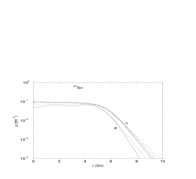
Figure 1: Four neutron and two proton densities for ¹²⁰Sn. Solid curves for SP model, dotted curves for ‘skin’ form, dashed curve for ‘halo’ form and dot-dashed curve for the ‘average’ form. All neutron densities have the same rms radius.

In a recent paper [8] Trzcińska et al. have suggested, based on analyses of strong interaction effects in antiprotonic atoms and of radiochemical data following $\bar{p}$ absorption on nuclei, that the difference between neutron and proton rms radii in nuclei depend on the asymmetry parameter $(N-Z)/A$ as follows:

$$r_{n}-r_{p}=-(0.04\pm 0.03)+(1.01\pm 0.15)\frac{N-Z}{A}~{}~{}{\rm(fm)}.$$ (2)

Addressing the question of the shape of the neutron density, they have concluded that a ‘halo’ rather than a ‘skin’ shape is preferred. These shapes are defined as follows: Assuming a two-parameter Fermi distribution both for the proton (unfolded from the charge distribution) and for the neutron density distributions

$$\rho_{n,p}(r)=\frac{\rho_{0n,0p}}{1+{\rm exp}((r-R_{n,p})/a_{n,p})},$$ (3)

then for the ‘skin’ form the same diffuseness parameter for the protons and the neutrons $a_{n}=a_{p}$ is used and the $R_{n}$ parameter is determined from the rms radius $r_{n}$. In the ‘halo’ form the same radius parameter $R_{n}=R_{p}$ is assumed for $\rho_{n}$ and for $\rho_{p}$, and $a_{n}^{\rm h}$ is determined from $r_{n}$. We also use an ‘average’ option where the diffuseness parameter is set to be the average of the above two diffuseness parameters, namely, $a_{n}^{\rm ave}=(a_{p}+a_{n}^{\rm h})/2$ and the radius parameter $R_{n}$ is determined from the rms radius $r_{n}$. To allow for different values of $r_{n}-r_{p}$ we have used Eq. (2) but with variable slope parameter, where, e.g. a slope of 1.5 fm correspons to the average behaviour of results of relativistic mean field (RMF) calculations [6, 9].

Figure 1 shows examples of densities used in the present work. The single-particle (SP) densities are described in [2]. The various neutron densities have the same value of $r_{n}$, as given by RMF calculations. Note that where the densities are well below 10% of their central values the neutron densities are significantly larger than the proton density.

3 Results

Fits were made to 90 data points using a variety of shapes of nuclear densities and values of $r_{n}$ as described in the previous section. Finite range was also introduced as an option, where the nuclear densities have been folded with a Gaussian, separately for the real and for the imaginary potentials, such that the densities in Eq. (1) are replaced by ‘folded’ densities

$$\rho^{F}(r)~{}~{}=~{}~{}\int d{\bf r}^{\prime}\rho({\bf r}^{\prime})\frac{1}{\pi^{3/2}\beta^{3}}e^{-({\bf r}-{\bf r^{\prime}})^{2}/\beta^{2}}~{}~{}.$$ (4)

Table 1 summarizes the main features of the results. The columns marked ‘RMF’ were obtained with values of $r_{n}-r_{p}$ taken from results of RMF calculation [9] whereas the columns marked ‘$\bar{p}$’ are for $r_{n}-r_{p}$ due to Ref. [8]. In both cases the 2-parameter Fermi distribution was used for the proton and for the neutron densities. The column marked with SP is for both densities obtained by filling in levels in single particle potentials [2] with $r_{n}-r_{p}$ values from the RMF model. The shapes of the neutron distributions (‘ave.’, ‘halo’, ‘skin’) are as explained in the previous section. The top part of the table is for zero range interaction and the bottom part of the table is for finite range interaction with Gaussian range parameters $\beta_{R}$ and $\beta_{I}$ for the real and for the imaginary parts, respectively. From the values of $\chi^{2}$/N for the zero range fits it is seen that reasonable fits to the data can be achieved for all options except for the ‘RMF-halo’ variety. The increased values of $\chi^{2}$/N compared to results of analyses of the previous data [1, 2] reflect the improved accuracy and the additional information contained in the new data. The latter is observed in the lower part of the table where the need for a finite-range version of the $\bar{p}$-nucleus optical potential is self-evident. The values of $\chi^{2}$ and of $\chi^{2}$/N mean significant improvements in the fits compared to the zero-range results. The best values for $\chi^{2}$/N are close to what has been achieved in global fits to pionic atom data [6].

Table 1: Global fits to 90 antiprotonic atom points. ‘RMF’ and ‘$\bar{p}$’ stand for values of $r_{n}-r_{p}$ used. Top part is for zero-range potentials and bottom part for finite-range potentials with range parameters $\beta_{R,I}$.

		‘RMF’			‘$\overline{p}$ atoms’
	SP	ave.	halo	skin	ave.	halo	skin
$\chi^{2}$	296	338	689	242	240	310	249
$\chi^{2}/$N	3.3	3.8	7.7	2.7	2.7	3.5	2.8
Re$b_{0}$ (fm)	2.5(2)	2.6(2)	2.0(2)	3.4(2)	3.1(2)	2.7(2)	3.6(2)
Im$b_{0}$ (fm)	3.1(2)	2.8(2)	2.5(2)	3.1(2)	3.2(2)	3.1(2)	3.4(2)
$\chi^{2}$	221	203	209	219	206	202	235
$\chi^{2}/$N	2.5	2.3	2.3	2.4	2.3	2.2	2.6
Re$b_{0}$ (fm)	0.78(5)	1.20(7)	0.68(5)	1.11(5)	1.77(9)	1.34(7)	0.71(3)
Im$b_{0}$ (fm)	1.75(6)	1.74(8)	1.10(4)	2.8(1)	2.3(1)	2.0(1)	3.5(1)
$\beta_{R}$ (fm)	1.0	0.9	0.9	1.2	0.7	0.8	1.6
$\beta_{I}$ (fm)	1.2	0.9	1.3	0.6	0.7	0.8	0.6

Next we turn to the question of whether the data require the presence of an isovector term $b_{1}$ in the potential Eq. (1). Fits to the full data set of 90 points failed to produce any reduction in $\chi^{2}$ when such a term was introduced. In a separate calculation we have been able to obtain a non-zero value for the parameter $b_{1}$ when fits were made to only the data for the Sn isotopes, leading to $\chi^{2}$/N of 1.0 for these isotopes. However, applying that $b_{1}$ to the full data set resulted in a major deterioration of the fit, and a further global fit restored the results of Table 1 with $b_{1}$=0. This is not surprizing since antiprotonic atoms are sensitive to the nuclear density in the extreme outer regions of the nucleus where the neutron density is dominant. Explicit isospin effects are, therefore, hard to observe.

Another attempt to improve the agreement between zero-range calculations and experiment was made by introducing a $p$-wave term into the optical potential [1, 2], a term which is active mostly at the surface region. Starting with the zero-range version of the potential, the values of $\chi^{2}$ could be reduced from those of the upper part of Table 1 to those of the lower part, but with $p$-wave parameters which depended critically on the choice of shape for the neutron distribution. Including in addition finite-range folding failed to further improve the fits.

In conclusion, global analyses of most of the data from PS209 reveal a need to improve on the previously successful zero-range $s$-wave isoscalar $\bar{p}$-nucleus optical potential. Including an isovector term is not required by the data nor is a $p$-wave term recommended at our present state of knowledge, although it undoubtedly improves the fits to the data when the zero-range form is used. The use of a finite-range interaction in the optical potential is definitely required by the data. Assuming that the values of the differences between rms radii $r_{n}-r_{p}$ are, on the average, between those advocated in Ref. [8] and those predicted by RMF calculations [9], and assuming the shape of the neutron distributions is between those described by the ‘skin’ and by the ‘average’ prescriptions, we then recommend the values Re$b_{0}$ = 1.3$\pm$0.1 fm, Im$b_{0}$ = 1.9$\pm$0.1 fm, with $\beta_{R}$ = $\beta_{I}$ = 0.85 fm within the folding expression Eq. (4).

References

- [1] C.J. Batty, E. Friedman and A. Gal, Nucl. Phys. A 592 (1995) 487.
- [2] C.J. Batty, E. Friedman and A. Gal, Phys. Rep. 287 (1997) 385.
- [3] A. Trzcińska et al., Nucl. Phys. A 692 (2001) 176c.
- [4] R. Schmidt et al., to be published.
- [5] B. Kłos et al., to be published.
- [6] E. Friedman and A. Gal, nucl-th/0302038.
- [7] H. De Vries et al., At. Data Nucl. Data Tables 36 (1987) 495.
- [8] A. Trzcińska et al., Phys. Rev. Lett. 87 (2001) 082501.
- [9] G.A. Lalazissis et al., At. Data Nucl. Data Tables 71 (1999) 1.